Voting with Their Feet?

Policy Research Working Paper 7047

Voting with Their Feet?

Access to Infrastructure and Migration in Nepal

Forhad Shilpi Prem Sangraula

Yue Li

Development Research Group

Agriculture and Rural Development Team

WPS7047

Public Disclosure Authorized Public Disclosure Authorized Public Disclosure Authorized Public Disclosure Authorized

Abstract

The Policy Research Working Paper Series disseminates the findings of work in progress to encourage the exchange of ideas about development issues. An objective of the series is to get the findings out quickly, even if the presentations are less than fully polished. The papers carry the names of the authors and should be cited accordingly. The findings, interpretations, and conclusions expressed in this paper are entirely those of the authors. They do not necessarily represent the views of the International Bank for Reconstruction and Development/World Bank and its affiliated organizations, or those of the Executive Directors of the World Bank or the governments they represent.

Policy Research Working Paper 7047

This paper is a product of the Agriculture and Rural Development Team, Development Research Group. It is part of a larger effort by the World Bank to provide open access to its research and make a contribution to development policy discussions around the world. Policy Research Working Papers are also posted on the Web at http://econ.worldbank.org.

The authors may be contacted at fshilpi@worldbank.org.

Using bilateral migration flow data from the 2010 popu- lation census of Nepal, this paper provides evidence on the importance of public infrastructure and services in determining migration flows. The empirical specification, based on a generalized nested logit model, corrects for the non-random selection of migrants. The results show that migrants prefer areas that are nearer to paved roads and have

better access to electricity. Apart from electricity's impact on

income and through income on migration, the econometric

results indicate that migrants attach substantial amenity

value to access to electricity. These findings have important

implications for the placement of basic infrastructure proj-

ects and the way benefits from these projects are evaluated.

Voting with Their Feet? Access to Infrastructure and Migration in Nepal

Forhad Shilpi, Prem Sangraula, Yue Li

JEL classification: O18, R13, R23

Key words: Migration, Public Goods, Income Effect, Amenity Value

Introduction

Do migrants respond to di¤erences in access to public goods and services in addition to income prospects of potential destinations? The income di¤erence between the origin and the destination is the primary factor driving migration in the existing literature on migration (Greenwood (1975) and Borjas (1994), Lall, Selod and Shalizi (2006)). Along with income, recent literature has also highlighted the importance of migration costs as well as migrants’ networks in determining migration ‡ows. How provision of public goods and services may in‡uence migration in poorer developing countries remains sparsely studied. This issue is however important in these countries where provision of public goods varies widely across areas. In a Tiebout (1956) sorting model, such disparity in the provision of public goods such as roads, electricity, schools, hospitals, etc. should induce people to "vote with their feet" and to migrate to areas with better access to these infrastructures and services.

From a policy perspective, it is important to know how migration responds to the provision of public goods in developing countries for a number of reasons. First, regions within a typical developing country are usually characterized by stark di¤erences in poverty and welfare. Households with poorer attributes such as low levels of education, skills and assets are frequently observed to live in poor areas that are characterized by lack of public infrastructure and services (Shilpi(2011), Dudwick et al. (2011), World Development Report (2009), Kanbur and Venables (2005), Jalan and Ravallion (2002), Ravallion and Wodon (1999)). If migrants do respond to income as well as provision of public infrastructure and services, then migration can act as a powerful instrument in mitigating regional di¤erences in welfare. Second, di¤erential costs of provision of infrastructure and services along with a hard budget constraint often force governments in developing countries to prioritize placement of these public goods. If people do migrate to gain better access to public goods, then the government may be able to rely more on cost considerations to prioritize their placement. Finally, migration in response to public goods and services also has important implications for the way the bene…ts of public investment are evaluated. A typical evaluation strategy

1Bayoh, Irwin and Haab (2006) …nds that central city’s inferior public goods, most notably school quality, play a dominant role in pushing households in the USA metropolitan cities to suburban locations.

of relying on variations in key outcomes such as income or household expenditure across areas with and without public goods would seriously underestimate the bene…t of the project. This is because migration in response to a new public good reduces the di¤erences in these outcomes across areas. Using census data from Nepal, this paper provides evidence on the extent to which access to public goods and services in‡uences bilateral migration ‡ow across areas.

The determinants of bilateral migration have been analyzed mostly in the context of international migration (Grogger and Hanson (2011), Ortega and Peri (2013)) and inter-regional migration (Ghatak, Mulhern and Watson (2008), Andrienko and Guriev (2004)).

This literature however focuses primarily on income and migration costs as determinants of migration ‡ow. A recent literature examines how migrants’

choice of destination is in‡uenced by locational attributes including the state of public infrastructure and services. For a relatively richer developing country – Brazil – Lall, Timmins and Yue (2009) …nd that poor migrants are willing to accept lower wages to achieve access to better services while richer migrants are in‡uenced only by income di¤erences.

Fafchamps and Shilpi (2013) …nd a statistically signi…cant and numerically large e¤ect of access to paved roads on migrants’destination choice in Nepal: migrants prefer a destination that is closer to a paved road. While contributing to this literature, the analysis in this paper di¤ers from the above papers in a number of ways. Instead of focusing on the destination choice of individual migrants, we analyze bilateral migration ‡ows across multiple sources and destinations. Our empirical speci…cation is derived from a model of utility maximization by the migrants proposed by Ortega and Peri (2013) and Grogger and Hanson (2011). We consider a generalized nested logit model where migrants …rst decide whether to migrate and then decide among the potential destinations. The advantage of this approach is that the resulting empirical speci…cation includes a correction term for the unobserved heterogeneity between migrants and non-migrants. The above mentioned papers (Fafchamps and Shilpi (2013), Lall, Timmins and Yue (2009)) in contrast side-stepped the issue of migrants’non-random selection

2For a survey of migration literature, please see Greenwood (1975) and Borjas (1994).

3For example, a Brazilian minimum wage worker earning R$7 an hour was willing to pay R$420 a year to have access to better health services, R$87 for a better water supply, and R$42 for electricity.

by focusing on the choice of destination conditional on migrating. More importantly, we make a distinction between the productivity and amenity values of basic infrastructure and services. For instance, access to electricity allows …rms to automate production, shifting the production possibility frontier ("productivity e¤ect"). It also helps households to carry out essential chores e¢ ciently and to enjoy leisure more fully ("amenity e¤ect"). We develop a strategy to uncover the amenity values of infrastructure and services. The strategy relies on a two-stage estimation procedure in which a canonical migration model –ignoring access to infrastructure and services – is …tted at the …rst stage. The …rst stage estimation thus allows income to capture the productivity e¤ect of the public goods. To the extent these goods are targeted to more productive areas, income in the …rst stage estimation picks up that placement e¤ect also. In the second stage, the residual from the …rst stage is regressed on measures of access to infrastructure and services. By construction, this strategy provides conservative estimates of amenity values of public goods.

The empirical analysis of this paper utilizes the detailed migration information from the population census 2010 of Nepal. Due to the mountainous terrain of the country and limited agricultural potential in many areas, migration is an important livelihood strategy for the Nepalese people. The rough terrain makes the provision of basic infrastructure very di¢ cult with the outcome that large parts of the country are not well served by transport infrastructure. Geographical coverage of electri…cation remains rather low, serving only a third of rural households. In terms of access to infrastructure and services as well as stage of economic development, Nepal is comparable to many Sub-Saharan African countries. The large geographical variations in access to basic public goods along with vibrant migration ‡ows make Nepal particularly suitable for our study.

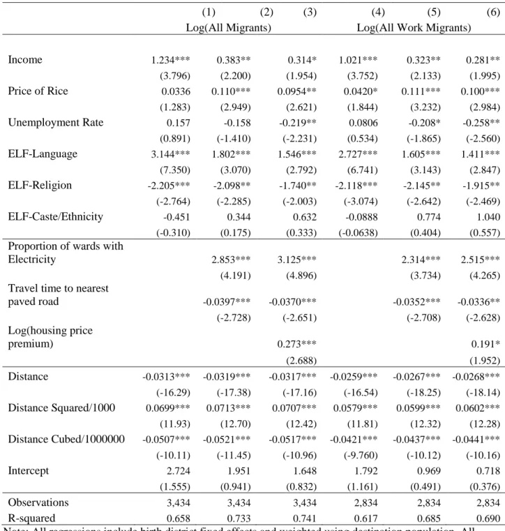
When a standard migration model is …tted, our empirical results con…rm the common …ndings of the

migration literature that income and distance between source and destination are the two most important

determinants of bilateral migration ‡ow. Consistent with the …ndings of Fafchamps and Shilpi (2013),

we …nd that when measures of access to basic public goods are added as regressors, the magnitude of the

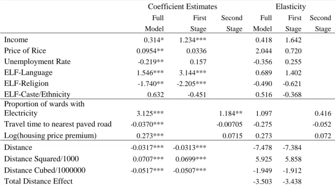
income coe¢ cient declines substantially though it still remains statistically signi…cant. This result con…rms

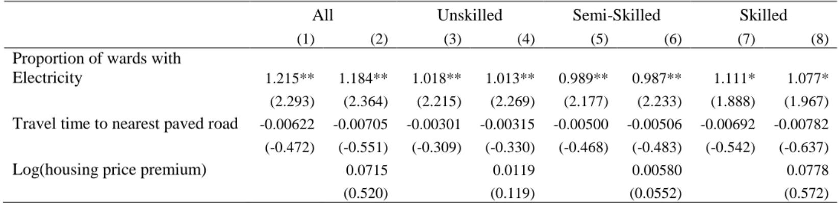
that the income coe¢ cient in a standard migration model is likely to be biased upward. Our results show that access to electricity and paved roads are important determinants of migration: migrants prefer areas with better access to electricity and paved roads. The results from the two-stage estimation procedures indicate that migrants attach substantial amenity value to access to electricity as well. Moreover, we

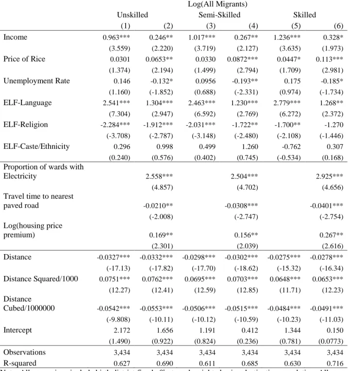
…nd that migrants of di¤erent skill levels (primary, secondary and tertiary education level) attach similar amenity values to access to electricity. Thus better access to electricity attracts migrants not only because it brightens their income prospects but also because it o¤ers better quality of life to them.

The rest of the paper is organized as follows. The conceptual framework and empirical speci…cation are presented in Section 2. Section 3 discusses the data. Section 4, organized in subsections, presents the empirical results. Section 5 concludes the paper.

2.Conceptual Framework 2.1 The Model

We start from a simple model of migration where an individual makes a utility maximizing migration decision among multiple destinations within the country. Individual h in her place of residence s decides whether to stay at s or to migrate to any of i 2 I = f 1; :::; N g : Let utility of individual h in location i be denoted U

. Following the literature, we assume that utility U

is a function of the income y

(or consumption) that the individual can achieve in location i, of the prices p

he or she faces, and a vector of location-speci…c amenities A

(Bayoh, Irwin and Haab, 2006). The utility from migrating to a given destination i depends on the migrant’s utility from income and amenities suitably adjusted for prices [u

(y

; A

; p

)] and on the costs C

of moving from s to i. Following Grogger and Hanson (2008) and Ortega and Peri (2009), we make a distinction between factors that are shared by all migrants from the same origin and to the same destination, and individual speci…c factors. The utility in destination i can be expressed as:

U

=

= u(y

; A

; p

) g(C

)

(1)

where

is an origin-destination speci…c term shared by all individuals migrating from s to i and

is the individual migrant speci…c term. u

(y

; A

; p

) is the expected utility of individual h in destination i.

The expected permanent income of individual h in destination i is the average income y

: In the empirical estimation, we allow di¤erences in incomes for workers of di¤erent skill levels. The expected utility in the destination depends also on the services and amenities available there along with the cost of living. This is important particularly for internal migration where individuals and households may move not only to capture income gain but also to avail themselves of better services and amenities – for instance better schools or health services –at destination. Similarly, C

is the average cost of migration from s to i. The cost term C

captures the physical distance between origin and destination. It also re‡ects costs incurred by individuals due to social distances (e.g. cultural, ethnic and language di¤erences) between the origin and destination.

We assume that u is an increasing function of y

; and A

; and a decreasing function of p

: We assume that g is an increasing function of C

: Following Grogger and Hanson (2008), we assume that both u and g are approximately linear functions. In the case of no migration, the average expected utility is:

U

= y

+ A

p

where ; and are positive constants. The utility from locating in i can be expressed as:

U

= y

+ A

p

C

(2)

where > 0 is a parameter. The individual speci…c term

denotes the idiosyncractic parts of the utility and cost associated with migration by individual h. There is now substantial evidence that migrants may be substantially di¤erent from non-migrants in terms of their ability, risk aversion and preferences.

Following Ortega and Peri (2009) we assume that:

h

si

= (1 )"

for i = s (3)

=

+ (1 )"

for i 6 = s

where "

is iid following an (Weibul) extreme value distribution.

is an individual speci…c term that a¤ects migrants only and its distribution is assumed to depend on 2 [0; 1). Given that "

has an extreme value distribution, then

has also an extreme value distribution (Cardell (1991). The migrant speci…c term

does not depend on destination and can be thought of capturing the di¤erences in preferences for migration.

Ortega and Peri (2009) show that utility maximization under the distributional assumptions leads to the following condition:

ln S

ln S

ln S

= [y

y

] + [A

A

] [p

p

] C

(4)

where S

= m

=n

; S

= (n

P

m

)=n

;and S

= m

= P

m

: n

is the total native born population of s; m

is the migrants born in s and gone to destination i; and

P

m

is the total migrants from s to all possible destinations. S

and S

are the share of migrants to location i in total native born population of s and total migrants from location s respectively. S

is the share native born population in s who chose to stay in s. The expression in equation (4) is very similar to an expression under standard logit formulation if = 0: The term in equation (4) corrects for the di¤erences in utility (due to income, amenity, prices and costs) between migrants and non-migrants (Ortega and Peri (2009)).

Subsitutiting for shares and solving for the logarithm of migration ‡ow (ln m

), equation (4) can be re-written as:

ln m

=

y

+

A

p

C

+

+

(5)

where

is the zero-mean measurement error,

is the origin …xed e¤ects and

=

;

=

;

=

1

; and

=

. In the standard logit formulation ( = 0); the …xed e¤ects account for share of the stayers in the population along with income, amenity and prices at the origin [

= ln(n

P

m

)].

When migrants di¤er systematically from non-migrants in preference and ability ( 6 = 0);the …xed e¤ects include a correction term (

ln

P

m

) for the average unobserved heterogeneity between migrants and non-migrants as well.

We estimate the speci…cation in equation (5) for bilateral gross migration ‡ows among districts in Nepal.

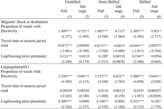
Following Grogger and Hanson (2011), we analyze sorting of migrants across destinations. Speci…cally, we analyze the variations in the skill mix of migrants to di¤erent destinations. We de…ne three groups of migrants in terms of their education level: those with (i) less than primary education, (ii) education between primary and secondary levels and (iii) above secondary level.

ln m

=

y

+

A

p

1

C

+

+

; for j = 1; 2; 3 (6)

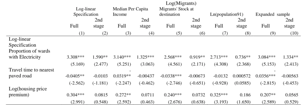
where j represents the education levels of migrants. The speci…cations in equations (5) and (6) are based on a linear utility and migration cost functions. A linear formulation can be interpreted as monetary income and cost whereas a log-linear speci…cation would imply as log income and time cost (Ortega and Peri (2013)). We performed estimation using both linear and log linear speci…cations.

Equations (5) - (6) are the basis of our main empirical estimation. A number of things are worth noting in the estimation of equations (5-6). First, when su¢ cient numbers of migrants come to a destination, it is expected to have general equilibrium e¤ects on wages, incomes and access to services and amenities.

This would generate a potential endogeneity bias due to the fact that income and amenities in a destination resulted in part from the decision of many migrants to locate there. To eliminate this bias, we use lagged explanatory variables. More precisely, let T be the period for which we have information on explanatory variables and T + t the period at which we observe migrants. Migrants are de…ned as those who migrated

4The e¤ect could be negative – e.g., congestion – or positive – e.g., agglomeration externalities.

between T and T +t whereas explanatory variables come from period T: Limiting the set of migrants in this fashion ensures that migration decisions are based only on information available prior to migration. Second, bilateral migration ‡ows between districts are not always positive. While our main estimation focused on districts with positive migration ‡ows, we also checked the robustness of our results for the sample which included districts with no migration ‡ows. We weight observations by destination population which corrects for potential heteroskedasticity of measurement error. The standard errors are clustered by destination districts to account for within (destination) district correlation of errors.

2.2 Empirical Speci…cation

The basic empirical speci…cations estimated from the data augment equations (5) and (6) with additional explanatory variables, leading to the following estimating equations:

ln m

=

y

+

A

p

C

+

Z

+

+

(7) ln m

=

y

+

A

p

C

+

Z

+

+

; for j = 1; 2; 3 (8)

where Z

is a vector of locational attributes of destination i. The Z

vector includes controls for social proximity between source and destination in terms of language, religion and ethnicity. Following standard practice in the literature, we also include a measure of the unemployment rate as a control.

Suppose

=

= 0, then equations (7 and 8) have the speci…cations that are comparable to speci…ca- tions derived from the standard model of determination of migration ‡ows when migrants’preferences for better access to public goods and services are ignored. For simplicity, suppose, y

and A

are uncorrelated with rest of the explanatory variables in the above equations and (

6 = 0;

6 = 0):We estimate equation (7) ignoring A

: The estimated coe¢ cient of income in this case is:

1

= ^

+ ^

(9)

where

is the estimated income coe¢ cient when A

is ignored and ^

and ^

1

are the estimated income and amenity/public goods coe¢ cients from the full speci…cation (equation 7) and is the correlation between y

and A

: Since income tends to be higher in areas with better public goods, > 0: The income coe¢ cient (

) thus overestimates the in‡uence of income di¤erences on migration ‡ow (^

) when migrant’s preference for public goods is ignored.

The positive correlation between income and public goods means that part of the preference for public goods is due to a preference for higher income. Some of the basic public goods such as roads and electricity have not only direct productivity and hence income e¤ect but also amenity values as they make life easier for households. To explore the amenity value of these goods and services, we utilize a two-stage procedure.

At the …rst stage, we …t a standard migration model ignoring public goods, which allows income to pick up the productivity e¤ect of public goods and services. At the second stage, the residual from the …rst stage is regressed on the explanatory variables representing access to public goods and services. Similar to equation (9), it follows that:

1

= ^

^

where

is the estimate of

from the second stage regression.

thus provides an estimate of the amenity value of public goods and services to migrants.

3. Data

The empirical analysis in this paper draws data from various sources: the population censuses of 2000 and 2010 and the Nepal Living Standard Survey 2002/3. The migration data are collected using the census long form for about 15 percent of the total population. This questionnaire collected information on district of current residence, district of residence 5 years prior to the census, and district of origin. Detailed information is also available on gender, age, education, religion, language spoken, ethnicity and motive for migration. This rich data-set is used to de…ne the gross bilateral migration ‡ows across districts.

5Nepal is divided into 75 districts.

The 15 percent sample of population census covers approximately 4.02 million individuals in 740,749 households. Because of our focus on adult migration, we restrict our attention to adults of age 15 and above. Of the 4.04 million individuals, about 35 percent are children below the age of 15 years. Among the adult population (about 2.65 million), about 18.7 percent are living in a district other than their district of birth. Among the migrants, 34 percent have moved in the six years preceding the census, that is, in the period between the 2002/3 NLSS and 2010 census. A large fraction of these individuals have moved for reasons other than work. Marriage is the dominant reason for moving among women (40 percent); study is the dominant reason for moving among children and youths (52 percent). In contrast, of the adult males who migrated during the last 6 years, 54 percent moved for work reasons. We estimate the migration

‡ows among districts using the census data and appropriate population weights. We de…ne two types of migrants: work migrants who moved to seek employment, and all migrants including work migrants as well as those who moved for non-work related reasons. All estimations are carried out for both of these samples.

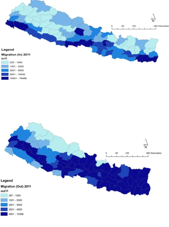
Figure 1 shows the geographical distribution of migrants in terms of district of residence and origin.

As apparent from Figure 1, a small number of destination districts have a high proportion of migrants. In contrast, districts of origin are distributed widely across the country. This re‡ects the fact that much of the migration is from rural areas to towns and cities. Indeed more than 90 percent of the migrants come from rural areas, and more than half of them migrated to an urban area. The same migration pattern is observed for work migrants.

While the census provided information about migration, it did not collect any information on income, prices and access to services and amenities. We utilize a nationally representative survey of households – the Nepal Living Standard Survey 2002/3 –to derive these explanatory variables. To estimate the average income level in a district i, we ran a regression of the following speci…cation:

y

=

+ x

+ v

where y

is the log of income of household h residing in district i,

is the district …xed e¤ects, and x

is a vector of household level explanatory variables and v

is the residual term. The regression includes household size and composition (number of adult males, females and children) as explanatory variables as larger households with more adults tends to earn more income and consume more; omitting them would overestimate incomes in districts where households are larger, e.g., rural districts. Other household characteristics are not included because they could possibly be a¤ected by migration. The estimated ’s provide of average district income for all households. We also included controls for di¤erent education levels to estimate education premia. Incomes for di¤erent skill categories are then computed using the education premia.

In the empirical analysis, migration costs are captured by geographical and social distances. For ge- ographical distance between districts, we utilize the arc distance between the district of origin and each possible district of destination, computed from the average longitude and latitude of each district.

We expect the cost and risk of migration to increase with physical distance. Social distance captures the e¤ect of migration networks which are found to be important in determining migration ‡ow ( Munshi (1993), Beaman (2012)). Social distance is measured by the index of ethno-linguistic fractionalization (ELF). The ELF index measures the probability that two individuals taken at random belong to the same ethnic or linguistic group. We estimated ELF for each district using the method suggested by Alesina and La Ferrara (2005). The ELF measures are de…ned for religious, linguistic and ethnic-caste groups using data from the 2000 population census. We computed the district level unemployment rate from the census 2000 data.

Instead of using the share of households with electricity, we construct a measure of electricity connection which does not depend directly on household income. We compute the share of wards – the smallest administrative unit in Nepal – that had electricity connection among all wards in a district using census

6The average longitude and latitude of a district are obtained as a weighted average of the longitude and latitude of all the VDC’s in the district, where the population of each VDC serves as weight.

2000 data.

This de…nition of access to electricity avoids the correlation with income that would have resulted from the ability of households with higher incomes to get electricity connection had the access variable been de…ned at the household level. As a measure of access to markets and other services (schools, hospitals, etc.), we estimated travel time to the nearest paved road from NLSS 2002/2003 data. Travel time to the nearest paved road correlates strongly and positively with other measures of access to services such as travel time to schools, hospitals, local markets and formal banks.

To control for price, we use price of rice. Rice is the most commonly consumed food item in Nepal and thus can be taken as a proxy for the price of common household goods. The NLSS 2002/3 collected information on the quantity and price paid for rice by individual households. We use these data to compute a unit price per kg.

We construct a measure of housing cost using data from the NLSS 2002/3 survey which contained a separate section on housing. The survey collected information on hypothetical and actual house rental values of each household together with house characteristics such as square footage, number and type of rooms, quality of materials, and the availability of various utilities. We use these data to construct a hedonic index of housing costs for each district. Let r

be the house rental price paid (or estimated) by household h in district i and let x

denote a vector of house characteristics. We estimate a regression of the form:

log r

= a

+ bx

+ e

where estimate of b a

provides a measure the housing cost premium in each district i. In the regression -omitted for the sake of brevity –many of the house characteristics are signi…cant with the expected sign, e.g., larger, better built houses with better in-house amenities are worth more. District price di¤erentials are large and jointly signi…cant. Since the dependent variable is in log form, b a

measures the housing cost premium in each district.

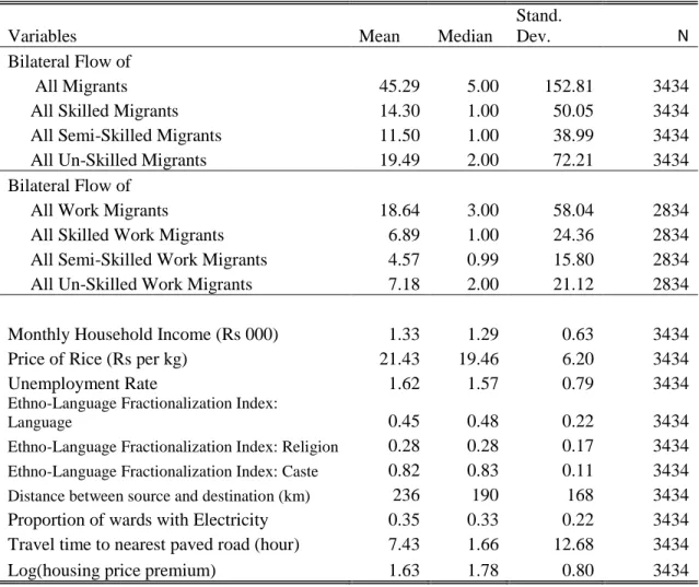
Table 1 reports the summary statistics for the dependent and explanatory variables. On average about

7There are more than 35 thousand wards in 75 districts in our census long form sample.

45 people migrated between a source-destination pairs. The number of work migrants is smaller –about 19 people. Migration appears to be concentrated at the two ends of the skill distribution: both unskilled (up to primary education) and skilled (above secondary education) tend to migrate at a higher propensity relative to semi-skilled workers (above primary but up to secondary education). This is true for work migration also.

This pattern is consistent with the pattern observed for international migration into OECD countries. The propensity to migrate into OECD countries is lower at the semi-skilled level (see Table 1 in Grogger and Hanson (2011)). The median arc distance between source and destination is about 190 km. The average travel time to the nearest paved road is about 7.4 hours indicating relative scarcity of paved roads in Nepal.

A large proportion of the country had no electricity connection in 2000, as only a third of the wards in a district reported to have electricity connection. The ELF measures show that Nepal is characterized by low religious diversity but by high ethno-caste diversity. The summary statistics of all other explanatory variables are also reported in Table 1.

4. Empirical Results

The initial set of regression results using the speci…cation in equation (7) are reported in Table 2. All regressions reported in this paper included birth district …xed e¤ects. All regressions are also weighted using destination district population, and all standard errors are clustered at the destination district level to account for any within district error correlations.

4.1. Determinants of Bilateral Migration Flow

We start with the simplest speci…cation which corresponds to the standard speci…cation estimated for bilateral migration ‡ow particularly in the context of international migration (Grogger and Hanson (2011), Ortega and Peri (2013)). The estimation is carried out for two samples: all migrants, and work migrants.

The results for this speci…cation are reported in columns 1 and 4 for the all migrant and work migrant samples, respectively. Consistent with the overwhelming evidence from the migration literature, migration

‡ow appears to be associated positively with income at the destination relative to that at source. The

income coe¢ cients (columns 1 and 4) are quite precisely estimated. The estimated income coe¢ cient for the

all migrants sample is slightly larger in magnitude than that for the work migrant sample but the hypothesis that the two income coe¢ cients are equal cannot be rejected even at the 20 percent signi…cance level. We introduced up to cubic terms of distance between source and destination, and all three terms are highly statistically signi…cant in explaining variations in migration ‡ow in both samples. The signs of the distance coe¢ cients are consistent with a priori expectation: migration ‡ow declines with an increase in distance between source and destination. Among other explanatory variables, the ELF measures for language and religious diversity have statistically signi…cant coe¢ cients though with opposite signs. The estimated coe¢ cients imply that migration ‡ow to a destination increases with language diversity but decreases with religious diversity and is not signi…cantly associated with ethno-caste diversity. These results are consistent with …ndings for Nepal reported in Fafchamps and Shilpi (2013). The estimation results show that rice price and unemployment rate do not appear to have statistically signi…cant association with migration

‡ow.

In the next speci…cation, we introduce two measures of public infrastructure and services: travel time to nearest paved road and percentage of wards electri…ed. The estimated coe¢ cients of these two variables have the expected sign (columns 2 and 5 in Table 2) and are statistically signi…cant at the 1 percent level.

The estimated coe¢ cients imply an increase in migration ‡ow to a destination with a decrease in travel time to paved roads and an increase in percentage of wards with electricity connections. Introduction of these two variables led to a substantial decline in the magnitudes of income coe¢ cients: they are now about one third of their respective magnitudes in columns 1 and 4. This con…rms our a priori expectation that areas with better access to infrastructure and services are also areas with higher incomes. Despite smaller magnitudes, income is still statistically signi…cant in both the all and work migrants samples.

It is worth noting that the measures of access to public infrastructure and services (travel time to paved

road and percentage of wards electri…ed) are de…ned from the NLSS 2002/3 and census 2000 data, whereas

migration ‡ow is de…ned over the period 2004 to 2010. Thus for the migration ‡ow under consideration,

measures of access to public goods are pre-determined. This helps us to avoid the problem of potential

reverse causation where migration could induce investment in public goods. One remaining concern with the estimated coe¢ cients of access to public goods and services is that they may be picking up the e¤ect of unobserved locational heterogeneity. To redress this issue, we note that in a Roy-Roback model of locational sorting, housing price captures the amenity/dis-amenity value of all location characteristics.

As noted by Bayer and Ross (2009), housing price can be taken as a summary measure of the relative attractiveness of an area. We introduce log of housing price premium as a control for unobserved locational heterogeneity where housing price premium estimates come from the NLSS 2002/3. The results from these augmented speci…cations are reported in columns 3 and 6 for the all migrant and work migrant samples, respectively. The estimated coe¢ cients of housing price premium are positive and statistically signi…cant in both samples suggesting that unobserved locational heterogeneity may be important in determining migration ‡ow. The estimates imply that areas with a higher housing price premia tend to receive higher in‡ow of migrants in subsequent periods. The estimates of income coe¢ cients have now become somewhat smaller in magnitudes. The same is true for the absolute magnitudes of access to paved roads coe¢ cients.

The magnitudes of coe¢ cients of access to electricity on the other hand have increased slightly. More importantly, none of the estimates are statistically signi…cantly di¤erent from their respective magnitudes in columns 2 and 5. This suggests that the correlations between unobserved heterogeneity on the one hand and access to paved road and electricity on the other hand are not strong enough to cause any substantial bias in the estimates of coe¢ cients of the latter variables.

Among the other explanatory variables, we …nd that unemployment rate has the expected negative sign when controls for access to paved road and electricity, and housing price premium are added to the regression. The coe¢ cient of rice price also becomes statistically signi…cant though with a positive sign.

Rice price is higher in urban areas compared with rural areas where it is grown because of transportation

cost. Rice price thus captures the fact that rural to urban migration is the predominant direction of

migration in Nepal. Finally, coe¢ cient estimates are statistically indi¤erent between the two samples. For

the rest of the paper, we thus limit our discussion to results from the full sample. In the next sub-section,

we explore if the results are di¤erent for migrants of di¤erent skills.

4.2. Determinants of Migration for Di¤erent Skill Levels

The determinants of migration ‡ow may be di¤erent for people of di¤erent skills. To the extent migrants with higher education come from relatively well-o¤ families, they may face lesser credit constraint in

…nancing their migration including the time spell during job search. On the other hand, poorer and unskilled migrants may be pushed out of their source due to adverse shocks and hence their migration may be less sensitive to income di¤erences. To explore these possibilities, we divide migrants into three groups in terms of their education level. Skilled migrants are those with higher than secondary education, and unskilled with primary or less education while semi-skilled belong to the middle group. We report the estimation results for the regression speci…cations in columns (1) and (3) of Table 2. The regression results are reported in Table 3.

The overall results for all three skill groups are consistent with those reported in Table 2. Some patterns are however worth noting. Income di¤erences between the source and destination seems to have relatively smaller in‡uence on unskilled migrants compared with semi- and skilled migrants, though income coe¢ cients are all positive and statistically signi…cant. The estimates of distance coe¢ cients on other hand display the opposite pattern: they are larger in absolute magnitudes for unskilled and semi skilled migrants compared with skilled migrants. This overall pattern is consistent with the expectations that many more of the unskilled migrants are push migrants and that because of credit constraint, they tend to migrate closer to their origin. Religious diversity –a factor that may relate inversely to migrants’social network – matters much less for the skilled migrants.

Access to paved roads and electricity have statistically signi…cant coe¢ cients in all three samples. The

estimated coe¢ cient is positive for access to electricity and negative for travel time to paved roads. The

magnitudes of the coe¢ cients are largest for the skilled migrants who are supposed to be least credit

constrained. According to the estimates, unskilled migrants are less sensitive to access to paved roads

compared with semi- and skilled migrants: the absolute value of the coe¢ cient of paved roads for unskilled

migrants is about half the size of that for skilled migrants. On other hand, skilled migrants are more sensitive to access to electricity compared with semi-skilled and unskilled migrants. The coe¢ cients of housing price premium have the expected positive sign and statistically signi…cant coe¢ cients in all three regressions. When these locational attributes are added to regressions, the overall pattern in the association between migration ‡ow and income, distance and other variables for the three groups of migrants remain the same. Consistent with our earlier …ndings, unemployment rate now has statistically signi…cant and negative coe¢ cients in all three regressions. As before, addition of these location characteristics to regressions leads to a signi…cant decline in the magnitudes of income coe¢ cients. While the income coe¢ cients are still statistically signi…cant and have positive signs, their magnitudes are about a third of what they are when access to public goods and housing prices were ignored. This again con…rms that income and these locational attributes are signi…cantly and positively correlated. To the extent access to paved roads and electricity contributes to higher income, their respective coe¢ cients capture not only their amenity value but also their productivity e¤ect re‡ected in higher income. In the following sub-section, we attempt to disentangle their amenity value.

4.3. Migration and Amenity Value of Public Goods and Services

To estimate the amenity value of public goods, we use a two-stage procedure. At the …rst stage, we estimate a standard migration model ignoring the di¤erences in the provision of electricity or paved roads across areas. This speci…cation thus corresponds to that in column 1 in Table 2, and columns 1, 3 and 5 in Table 3. As shown in equation 9, the coe¢ cient of income in the …rst stage regression picks up part of the e¤ect of access to public goods and services. At the second stage, the residual from …rst stage is regressed on the locational attributes. As the …rst stage regression purges the possible productivity e¤ect of public goods, the second stage estimates thus provide measures of their amenity value. Income in the …rst stage may pick up more than productivity e¤ect: it may capture part of amenity value that is correlated with productivity e¤ect. Thus second estimates can be considered as lower bound estimates of amenity values.

The second stage estimates are reported in Table 4. The estimates are given for the full sample as well

as for unskilled, semi-skilled and skilled migrants’ samples. For each sample, the estimates are reported for two speci…cations: one excluding housing price premium and the other including it. Regardless of the speci…cations, the estimates of coe¢ cients of access to electricity fall within a tight interval [0.987-1.215].

These estimates are also statistically signi…cant at 10 percent signi…cance level or less. The estimates of coe¢ cients of travel time to paved road have the expected negative signs but none of them are statistically or numerically signi…cant. The coe¢ cients of housing price premium are also not numerically or statistically signi…cant for any of sub-groups of migrants.

The estimates for access to electricity suggest that migrants do attach amenity value to it. Even after conditioning on income, migration ‡ows are greater to areas which have better access to electricity. The results in Table 4 also suggest no substantial variations in the way migrants of di¤erent skill types value access to electricity as an amenity. The estimates of coe¢ cients of access to electricity in Tables 2 and 3 fall within the interval of [ 2.5-3.12]. The estimates in Table 4 are much smaller in magnitude –roughly about 40 percent of magnitude of estimates in Tables 2 and 3. In other words, of all the migration that happens in response to access to electricity, 40 percent of those is perhaps due to electricity’s amenity value.

The estimates in Tables 2 and 3 suggested strong and negative association between bilateral migration

‡ows and travel time to paved road, the estimates in Table 4 show absence of a signi…cant association between these two variables. The strong and negative association between income and geographic isolation (measured here by travel time to paved road) is well noted in the case of Nepal (Fafchamps and Shilpi (2008) and (2013)). The lack of signi…cance of travel time to paved road in the second stage does not necessarily imply that migrants do not attach any amenity value to access to paved road. Rather it suggests that the correlations of travel time to paved road with income and with access to electricity are strong and that given those correlations, it is not possible to disentangle the productivity and amenity value of paved roads.

4.4. Robustness Checks

We perform a number of robustness checks. These checks are conducted for all di¤erent samples. To

avoid clutter, we report the estimates of the coe¢ cients of access to electricity, paved road and housing price

premium. We also report estimates from two regressions: a full model where all variables are introduced simultaneously; and the estimates from the second stage regression where …rst stage regression did not include any of the three variables of our interest. The full model thus corresponds to speci…cations whose results are reported in column 3 of Table 2 and columns 2, 4, and 6 of Table 3. The conditional estimates from second stage correspond to results reported in the even numbered columns of Table 4. We report the results for all migrants in Table 5.

The regression results reported so far come from speci…cations where income and distance variables are measured in levels. In most migration studies, these variables are often introduced in the logarithmic form.

The logarithmic form would imply a log-linear utility function which –according to Grogger and Hanson (2011) – could be mis-speci…ed leading to omitted variable bias. To avoid mis-speci…cation, we estimated the speci…cation consistent with the linear utility function where income and distance enter the regression equation linearly. In the …rst robustness check, we estimate the regression in log-linear form with both income and distance variables in logarithms. The estimates of parameters of our main interest from the full and conditional (second stage) regressions are reported in columns 1 and 2 of Table 5. The estimates are similar in sign and magnitudes to those reported in Tables 2 and 4.

In the next couple of robustness exercises, we address the issue of potential measurement errors in income

estimation. The district level income estimates come from the NLSS 2002/3 data. Income estimates from

household surveys typically involve measurement error though NLSS 2002/3 is a nationally representative

survey. To check whether our estimates are sensitive to alternative indicators of income, we conduct three

robustness checks: (i) Instead of average income adjusted for household size and composition, we use

median per capita income at the district level as our income variable. The resulting regression estimates

are presented in columns 3 and 4. (ii) While past income from household survey may provide information

about potential income at the destination, migrants may not have adequate information on potential income

in all di¤erent destinations. An important source of information about jobs and incomes for migrants is

the past migrants from the same area. We take past stock of migrants who migrated more than 6 years ago

normalized by destination population as an indicator size of migrants’network and add this as a regressor.

The results from these regressions are reported in columns 5 and 6. (iii) Incomes across geographical locations are found to be highly correlated with population with income being higher in more populated areas. Population density on the other hand is outcome of migration as well as state of public goods. To avoid reverse causation, we added log of population in 1991 as an additional regressor. The results are reported in columns 7 and 8 in Table 5. The introduction of later two variables (past migrants’ stock and population) renders income coe¢ cient smaller in magnitude and statistically signi…cant only at 10 percent level. However, the qualitative results with respect to access to electricity remain unchanged in all of the robustness exercises. When stock of past migrants or population in 1991 are added in the regressions, the magnitudes of coe¢ cients of electricity become somewhat smaller, yet they remain both numerically and statistically signi…cant. The results regarding the signi…cance of access to paved road as a determinant of migration ‡ow become much weaker when past migrants network or past population are added in the regressions. Similar to income, stock of past migrants and population seem to be highly and positively correlated with travel time to paved road. However, the results regarding its amenity value remains unchanged.

In the main regressions, we focused on the sample of all districts with positive migration ‡ows. In the next robustness check, we included all districts including those with zero migration ‡ow. The results are shown in the …nal two columns of Table 5. The results for this expanded sample is nearly indistinguishable to those reported in Tables 2 and 4.

We repeated the robustness checks for migrants of di¤erent skill levels. The results are similar to those

reported in Table 5. In the upper panel of Table 6, we report the results when stock of past migrants is

included as an additional regressor. The lower panel reports the results with log of 1991 population as

an additional regressor. The results are comparable to those for the full sample. Though the magnitudes

of coe¢ cients of access to electricity are somewhat smaller compared with those in Table 4, they are all

numerically and statistically signi…cant. As before, we …nd that coe¢ cients of travel time to paved road

become statistically insigni…cant when population is added as a regressor. In all other cases, migration

‡ow seems to respond signi…cantly with access to paved road in the full regression.

It is worth noting that population of a district captures the relative degree of urbanization as well:

districts with larger urban share also have higher population. Since urban areas di¤er distinctly from rural areas in terms of income and access to public goods, introduction of population in the regression leads to a substantial decline in the magnitudes of coe¢ cients of these variables. Thus inclusion of population as a regressor is likely to bias the estimates of income and public goods coe¢ cients downward. Same argument can be made about stock of past migrants. Our preferred speci…cations thus exclude these two variables.

4.5. Economic Signi…cance

The explanatory variables in the regressions are measured in di¤erent units and thus it is di¢ cult to compare the magnitudes of coe¢ cients of di¤erent variables. To provide an idea about the relative importance of di¤erent factors in determining migration ‡ows, we provide the estimates of the elasticities based on the estimated coe¢ cients which are reported in Table 7.

We computed elasticities for both the full model which included all explanatory variables simultaneously

and the two stage procedure which excluded access to paved road and electricity and housing price premium

from the …rst stage regression. In both models, distance between the source and destination is the most

important regressor in terms of the magnitude of its e¤ect on migration. In the full model, other important

factors in terms of magnitudes are access to electricity and rice price. Income is also important along with

language diversity and access to paved roads, but its magnitude is relatively small implying an increase

of migration ‡ow by about 0.4 percent in response to a one percent increase in income. When income is

allowed to pick up the e¤ect of infrastructure and services, we …nd income to be one of the most important

determinant of migration ‡ow next only to distance in terms of magnitude of e¤ect. Even after allowing

income to pick up part of the e¤ect of access to electricity, access to electricity still remains as an important

determinant of migration ‡ow. Interpreting the second stage coe¢ cient as capturing the amenity value,

the elasticity of migration with respect to electricity in the second stage con…rms that migrants do assign

considerable value to access to electricity as an amenity. Our …nding regarding access to electricity is consistent with that of Lall, Timmins and Yue (2009). However, unlike Lall, Timmins and Yue (2009) who

…nd access to electricity to be valued only by the poorer households, our results suggest that its amenity value does not vary across skill groups of migrants. This is perhaps due to the fact that access to electricity is still limited in Nepal with only a third of wards reporting to have access. In contrast, Brazil has nearly universal geographical coverage for electricity (97 percent of rural areas), and the access issue there is more of …nancial ability to get an electricity connection and paying bills.

5. Conclusions

In the standard new economic geography models, labor is assumed to be mobile in the medium to longer term (Fujita, Krugman and Venables (1999)). With labor mobility, any regionally targeted policy intervention in these models induces labor movement so as to restore spatial equilibrium. Evaluation of large public investment projects such as transportation, electri…cation and communication on the other hand tends to use spatial variations in outcomes and treatments to estimate returns while ignoring the labor mobility issue. In this paper, we provide evidence on the response of migration to public infrastructure and services using census and household data from a poor developing country, Nepal.

The empirical analysis of this paper incorporates several improvements over the existing literature on the determinants of internal and international migration. The standard model of migration –estimated mostly for international migration – tends to ignore the role of access to public goods and services in the migration decision. Our conceptual model and empirical estimation show that such model tends to over- estimate the importance of income in the determination of migration ‡ow due to the positive correlation between income and provision of public goods. Second, while the empirical studies focusing on migrants’

destination choice do pay attention to spatial di¤erences in the provision of public goods, they tend to

side-step the issue of migrants’ non-random selection. There is now a large literature that demonstrates

clearly that migrants tend to be di¤erent from non-migrants in terms of both observables and unobservables

(Gabriel and Schmitz (1995), Dahl (2002), Akee (2006), Mckenzie, Gibson and Stillman (2010)). Using

a nested logit model of utility maximization by the migrants – as suggested by Ortega and Peri (2013) – we derive an empirical speci…cation which corrects for the heterogeneity between migrants and non- migrants. Third, we make a distinction between the productivity and hence income e¤ect, and amenity value of basic infrastructure such as electri…cation. The income e¤ect arises from its direct e¤ect on

…rm and farm productivity whereas the amenity value derives from its use in household activities (e.g.

chores/studying/entertainment). Using the correlation between income and access to these public goods, we develop a strategy to provide conservative estimates of their amenity values.

The empirical results show that migrants prefer areas which are nearer to their birth place and have higher income, better access to electricity and paved roads, higher rice and housing prices and greater language diversity. Consistent with the …ndings of Fafchamps and Shilpi (2013), we …nd that when mea- sures of access to basic public goods are added as regressors, the magnitude of income coe¢ cient declines substantially though it still remains statistically signi…cant. This result con…rms that the income coe¢ cient in a standard migration model might be biased upward. We …nd some heterogeneity in the way income, distance and access to a paved road in‡uence migration for di¤erent skill groups: more skilled migrants are more responsive to income and access to paved road but less responsive to distance relative to unskilled migrants. The results from the two-stage estimation procedure indicate that migrants attach substantial amenity value to access to electricity. Migrants of di¤erent skill levels (primary, secondary and tertiary education level) appear to attach similar amenity values to access to electricity. The results suggest that better access to electricity attracts migrants not only for its positive productivity and income e¤ect but also for its amenity value.

The main …nding of this paper that migrants do respond to access to public goods has important im-

plications for the placement and evaluation of basic public infrastructure and services. While geographical

coverage of these public goods should be universal, budget constraints often force governments to prioritize

their roll out. Our empirical results suggest that governments can perhaps give more weight to cost con-

siderations in prioritizing the roll out. Our results also suggest that impact evaluation of public investment

should pay particular attention to spill-over e¤ects to non-treatment areas due to migration. Such spill-over e¤ects can in turn lead to substantial downward bias in the estimates of returns to public investment when its e¤ect on migration is ignored in the evaluation studies.

References

1. Akee, Randall K.Q., “Deciphering Immigrant Self-Selection: New Evidence from a Developing Coun- try,” Kennedy School of Government, Harvard University, Cambridge Mass., 2006 (mimeograph)

2. Andrienko, Y. and S. Guriev, 2004. "Determinants of interregional mobility in Russia: Evidence from panel data", Economics of Transition, Volume 12 (1) 2004, 1–27.

3. Bayoh Isaac, Elena G. Irwin and Timothy Haab, “Determinants of Residential Location Choice: How Important Are Local Public Goods in Attracting Homeowners to Central City Locations?,” Journal of Regional Science, 46(1), 97-120, February 2006.

4. Beaman, Lori A., 2012. “Social Networks and the Dynamics of Labor Market Outcomes: Evidence from Refugees Resettled in the US,” Review of Economic Studies, vol. 79(1), pages 128-161.

5. Bayer, P. and S. Ross, 2006, "Identifying Individual and Group E¤ects in the Presence of Sorting:

A Neighborhood E¤ects Application," NBER Working Papers 12211, National Bureau of Economic Research.

6. Borjas, George J., “The Economics of Immigration,” Journal of Economic Literature, 32(4), 1667- 1717, December 1994

7. Dahl, Gordon B., “Mobility and the Return to Education: Testing a Roy Model with Multiple Markets,” Econometrica, 70(6), 2367-2420, November 2002

8. Dudwick,N., K. Hull, R. Katayama, F. Shilpi and K. Simler, 2011. From Farm to Firm: Rural-Urban

Transition in Developing Countries, World Bank Direction in Development Series.

9. Fujita, Masahisa, Paul Krugman and Anthony J. Venables, The Spatial Economy: Cities, Regions, and International Trade, MIT Press, Cambridge and London, 1999

10. Gabriel, Paul E. and Suzanne Schmitz, “Favorable Self-Selection and the Internal Migration of Young White Males in the United States,” Journal of Human Resources, 30(3), 460-71, Summer 1995

11. Ghatak, S., A. Mulhern and J. Watson, 2008. "Inter-Regional Migration in Transition Economies:The Case of Poland", Review of Development Economics, 12(1), 209–222.

12. Greenwood, Michael J., “Research on Internal Migration in the United States: A Survey,” Journal of Economic Literature, 13(2), 397-433, June 1975

13. Grogger, Je¤rey and Hanson, Gordon H., 2011. "Income maximization and the selection and sorting of international migrants," Journal of Development Economics, vol. 95(1), pages 42-57, May.

14. Harris, John and M. Todaro, “Migration, Unemployment and Development: A Two-Sector Analysis,”

Amer. Econ. Rev., 60, 126-142, 1970

15. Jalan, Jyotsna and Martin Ravallion, 2002, “Geographic Poverty Traps? A Micro Model of Con- sumption Growth in Rural China,” Journal of Applied Econometrics, Vol. 17, p. 329-346.

16. Kanbur, R and A. Venables, 2005, Spatial Inequality and Development, Oxford University Press: New York.

17. Lall, Somik and Christopher Timmins, “Rural-Urban Migration: Successful Integration or just

"Bright Lights"? Evidence from Brazil and Mexico,” Department of Economics, Duke University, 2008 (mimeograph)

18. Lucas, Robert E. Jr, “Life Earnings and Rural-Urban Migration,” Journal of Political Economy,

112(1), S29-59, Feb. 2004

19. McKenzie, David, John Gibson and Steven Stillman, 2010. “How Important Is Selection? Experimen- tal vs. Non-Experimental Measures of the Income Gains from Migration,” Journal of the European Economic Association, vol. 8(4), pages 913-945.

20. Munshi, Kaivan, 2003. “Networks in the Modern Economy: Mexican Migrants in the US Labor Market,” Quarterly Journal of Economics, 118(2), 549-99, May 2003

21. Ortega, F. and G. Peri, 2013. “The E¤ect of Income and Immigration Policies on International Migration”. Migration Studies, Volume 1, page 1-28.

22. Ravallion, M and Q. Wodon, 1999,“Poor Areas or Poor People?” Journal of Regional Sciences, Vol.

39(4), p. 689-711.

23. Ravallion, Martin and Jyotsna Jalan, 1999, “China’s Lagging Poor Areas,” American Economic Review Papers and Proceedings, Vol. 89(2), pp. 301-305.

24. Roback, J, 1982,“Wages, Rents and Quality of Life,”Journal of Political Economy, vol. 90, p.1257-78.

25. Roy, A. D, 1951, “Some Thoughts on the Distribution of Earnings,” Oxford Economic Papers, vol.3, p. 135-46.

26. Shilpi, Forhad. 2011. “Mobility costs and regional inequality: Evidence from Bangladesh,” Journal of Globalization and Development, 2(1).

27. Tiebout, C. (1956), "A Pure Theory of Local Expenditures", Journal of Political Economy, 64 (5):

416–424,

28. World Development Report 2009. Reshaping Economic Geography, World Bank, Washington DC.

Figure 1: In and Out- Migration by districts in Nepal, 2011

Table 1: Summary Statistics

Variables Mean Median

Stand.

Dev. N

Bilateral Flow of

All Migrants 45.29 5.00 152.81 3434

All Skilled Migrants 14.30 1.00 50.05 3434

All Semi-Skilled Migrants 11.50 1.00 38.99 3434

All Un-Skilled Migrants 19.49 2.00 72.21 3434

Bilateral Flow of

All Work Migrants 18.64 3.00 58.04 2834

All Skilled Work Migrants 6.89 1.00 24.36 2834

All Semi-Skilled Work Migrants 4.57 0.99 15.80 2834

All Un-Skilled Work Migrants 7.18 2.00 21.12 2834

Monthly Household Income (Rs 000) 1.33 1.29 0.63 3434

Price of Rice (Rs per kg) 21.43 19.46 6.20 3434

Unemployment Rate 1.62 1.57 0.79 3434

Ethno-Language Fractionalization Index:

Language 0.45 0.48 0.22 3434

Ethno-Language Fractionalization Index: Religion 0.28 0.28 0.17 3434 Ethno-Language Fractionalization Index: Caste 0.82 0.83 0.11 3434

Distance between source and destination (km) 236 190 168 3434

Proportion of wards with Electricity 0.35 0.33 0.22 3434

Travel time to nearest paved road (hour) 7.43 1.66 12.68 3434

Log(housing price premium) 1.63 1.78 0.80 3434

Table 2: Determinants of Migration Flow: Regression Results

(1) (2) (3) (4) (5) (6)

Log(All Migrants) Log(All Work Migrants)

Income 1.234*** 0.383** 0.314* 1.021*** 0.323** 0.281**

(3.796) (2.200) (1.954) (3.752) (2.133) (1.995) Price of Rice 0.0336 0.110*** 0.0954** 0.0420* 0.111*** 0.100***

(1.283) (2.949) (2.621) (1.844) (3.232) (2.984) Unemployment Rate 0.157 -0.158 -0.219** 0.0806 -0.208* -0.258**

(0.891) (-1.410) (-2.231) (0.534) (-1.865) (-2.560) ELF-Language 3.144*** 1.802*** 1.546*** 2.727*** 1.605*** 1.411***

(7.350) (3.070) (2.792) (6.741) (3.143) (2.847) ELF-Religion -2.205*** -2.098** -1.740** -2.118*** -2.145** -1.915**

(-2.764) (-2.285) (-2.003) (-3.074) (-2.642) (-2.469)

ELF-Caste/Ethnicity -0.451 0.344 0.632 -0.0888 0.774 1.040

(-0.310) (0.175) (0.333) (-0.0638) (0.404) (0.557)

Proportion of wards with

Electricity 2.853*** 3.125*** 2.314*** 2.515***

(4.191) (4.896) (3.734) (4.265)

Travel time to nearest

paved road -0.0397*** -0.0370*** -0.0352*** -0.0336**

(-2.728) (-2.651) (-2.708) (-2.628)

Log(housing price

premium) 0.273*** 0.191*

(2.688) (1.952)

Distance -0.0313*** -0.0319*** -0.0317*** -0.0259*** -0.0267*** -0.0268***

(-16.29) (-17.38) (-17.16) (-16.54) (-18.25) (-18.14) Distance Squared/1000 0.0699*** 0.0713*** 0.0707*** 0.0579*** 0.0599*** 0.0602***

(11.93) (12.70) (12.42) (11.81) (12.32) (12.28) Distance Cubed/1000000 -0.0507*** -0.0521*** -0.0517*** -0.0421*** -0.0437*** -0.0441***

(-10.11) (-11.45) (-10.96) (-9.760) (-10.12) (-10.16)

Intercept 2.724 1.951 1.648 1.792 0.969 0.718

(1.555) (0.941) (0.832) (1.161) (0.491) (0.376)

Observations 3,434 3,434 3,434 2,834 2,834 2,834

R-squared 0.658 0.733 0.741 0.617 0.685 0.690

Note: All regressions include birth district fixed effects and weighted using destination population. All standard errors are clustered at destination district level. ELF: Ethno-Linguistic Fractionalization Index.

Robust t-statistics in parentheses

*** p<0.01, ** p<0.05, * p<0.1

Table 3: Determinants of Migration Flow by Skill Groups: Regression Results Log(All Migrants)

Unskilled Semi-Skilled Skilled

(1) (2) (3) (4) (5) (6)

Income 0.963*** 0.246** 1.017*** 0.267** 1.236*** 0.328*

(3.559) (2.220) (3.719) (2.127) (3.635) (1.973) Price of Rice 0.0301 0.0653** 0.0330 0.0872*** 0.0447* 0.113***

(1.374) (2.194) (1.499) (2.794) (1.709) (2.981)

Unemployment Rate 0.146 -0.132* 0.0956 -0.193** 0.175 -0.185*

(1.160) (-1.852) (0.688) (-2.331) (0.974) (-1.734) ELF-Language 2.541*** 1.304*** 2.463*** 1.230*** 2.779*** 1.268**

(7.304) (2.947) (6.592) (2.769) (6.272) (2.372) ELF-Religion -2.284*** -1.912*** -2.031*** -1.722** -1.700** -1.270 (-3.708) (-2.787) (-3.148) (-2.480) (-2.108) (-1.446)

ELF-Caste/Ethnicity 0.296 0.998 0.499 1.260 -0.762 0.307

(0.240) (0.576) (0.402) (0.745) (-0.534) (0.168)

Proportion of wards with

Electricity 2.558*** 2.504*** 2.925***

(4.857) (4.702) (4.656)

Travel time to nearest

paved road -0.0210** -0.0308*** -0.0401***

(-2.008) (-2.747) (-2.754)

Log(housing price

premium) 0.169** 0.156** 0.267**

(2.301) (2.039) (2.616)

Distance -0.0327*** -0.0332*** -0.0298*** -0.0302*** -0.0275*** -0.0278***

(-17.13) (-17.82) (-17.70) (-18.62) (-15.32) (-16.34) Distance Squared/1000 0.0751*** 0.0762*** 0.0695*** 0.0703*** 0.0648*** 0.0653***

(12.27) (12.41) (12.59) (12.85) (11.71) (12.23) Distance

Cubed/1000000 -0.0542*** -0.0553*** -0.0506*** -0.0515*** -0.0484*** -0.0491***

(-9.808) (-10.11) (-10.12) (-10.59) (-10.23) (-11.03)

Intercept 2.172 1.656 1.191 0.412 1.344 0.150

(1.490) (0.922) (0.824) (0.236) (0.781) (0.0773)

Observations 3,434 3,434 3,434 3,434 3,434 3,434

R-squared 0.627 0.690 0.611 0.685 0.630 0.716

Note: All regressions include birth district fixed effects and weighted using destination population. All standard errors are clustered at destination district level. . ELF: Ethno-Linguistic Fractionalization Index.

Robust t-statistics in parentheses

*** p<0.01, ** p<0.05, * p<0.1