Mesoscopic Modelling of Self- Propelled Particles or Active Matter C. Holm, Institut für Computerphysik, Universität Stuttgart

Mesoscopic Modelling of Self-

Propelled Particles or Active Matter

C. Holm, Institut für Computerphysik, Universität Stuttgart

http: www.icp.uni-stuttgart.de

Email: holm@icp.uni-stuttgart.de

• An active matter system can take energy from its environment and drive itself far from equilibrium

(S. Ramaswamy, Annu. Rev. Condens. Matter Phys. 1, 323–345)

• For an SPP this means it starts to move

• It can show interesJng single moJon or also cooperaJve behavior

What is Active Matter?

Falcon Attacks Clouds of starlings (BBC Youtube)

Travelling wave in Penguin Population (Ben Fabry, Erlangen)

Drosophila Embryio undergoing cell division (S. Streichan, UCSB)

Active Matter across the Length Scales

Acve ma(er is ubiquitous.

Molecular motors

Bacteria

Eukaryotes

Social insects

Birds & Fish

Mammals  

Biological Active Matter Across Scales

And it just exploded from there…

Taken from Scopus for ‘Acve Ma(er’ or ‘Self Propelled’.

Wake Up!

Tamás Vicsek et al., Phys. Rev. Le6. 75, 1226 (1995)

Novel Type of Phase Transi2on in a System of Self-Driven Par2cles

How the field started

these micromachines and nanomachines hold the promise of performing key tasks in an autonomous, targeted, and selec- tive way. The possibility of designing, using, and controlling microswimmers and nanoswimmers in realistic settings of operation is tantalizing as a way to localize, pick up, and deliver nanoscopic cargoes in several applications — from the targeted delivery of drugs, biomarkers, or contrast agents in health care applications (Nelson, Kaliakatsos, and Abbott, 2010; Wang and Gao, 2012; Patra et al., 2013; Abdelmohsen et al., 2014) to the autonomous depollution of water and soils contaminated because of bad waste management, climate changes, or chemical terroristic attacks in sustainability and security applications (Gao and Wang, 2014).

The field of active matter is now confronted with various open challenges that will keep researchers busy for decades to come. First, there is a need to understand how living and inanimate active matter systems develop social and (possibly) tunable collective behaviors that are not attainable by their counterparts at thermal equilibrium. Then, there is a need to understand the dynamics of active particles in real-life environments (e.g., in living tissues and porous soils), where randomness, patchiness, and crowding can either limit or enhance how biological and artificial microswimmers perform a given task, such as finding nutrients or delivering a nano- scopic cargo. Finally, there is still a strong need to effectively scale down to the nanoscale our current understanding of active matter systems.

With this review, we provide a guided tour through the basic principles of self-propulsion at the microscale and nanoscale, the development of artificial self-propelling microparticles

and nanoparticles, and their application to the study of far- from-equilibrium phenomena, as well as through the open challenges that the field is now facing.

II. NONINTERACTING ACTIVE PARTICLES IN HOMOGENOUS ENVIRONMENTS

Before proceeding to analyze the behavior of active particles in crowded and complex environments, we set the stage by considering the simpler (and more fundamental) case of individual active particles in homogeneous environments, i.e., without obstacles or other particles. We first introduce a simple model of an active Brownian particle, ¹ which will permit us to understand the main differences between passive and active Brownian motion (Sec. II.A) and serve as a starting point to discuss the basic mathematical models for active motion (Sec. II.B). We then introduce the concepts of effective diffusion coefficient and effective temperature for self- propelled Brownian particles, as well as their limitations, i.e., differences between systems at equilibrium at a higher temperature and systems out of equilibrium (Sec. II.C). We then briefly review biological microswimmers (Sec. II.D).

Finally, we conclude with an overview of experimental achievements connected to the realization of artificial micro- swimmers and nanoswimmers including a discussion of the principal experimental approaches that have been proposed so far to build active particles (Sec. II.E).

A. Brownian motion versus active Brownian motion

In order to start acquiring some basic understanding of the differences between passive and active Brownian motion, a good (and pedagogic) approach is to compare two- dimensional trajectories of single spherical passive and active particles of equal (hydrodynamic) radius R in a homogenous environment, i.e., where no physical barriers or other particles are present and where there is a homogeneous and constant distribution of the energy source for the active particle.

The motion of a passive Brownian particle is purely diffusive with translational diffusion coefficient

D _T ¼ k _B T

6πηR ; ð 1 Þ

where k _B is the Boltzmann constant, T is the absolute temperature, and η is the fluid viscosity. The particle also undergoes rotational diffusion with a characteristic time scale τ _R given by the inverse of the particle ’ s rotational diffusion coefficient

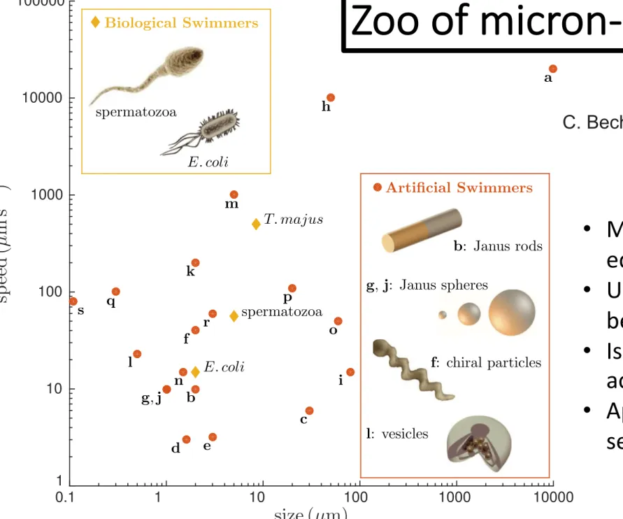
FIG. 1. Self-propelled Brownian particles are biological or man- made objects capable of taking up energy from their environment and converting it into directed motion. They are microscopic and nanoscopic in size and have propulsion speeds (typically) up to a fraction of a millimeter per second. The letters correspond to the artificial microswimmers in Table I. The insets show examples of biological and artificial swimmers. For the artificial swimmers four main recurrent geometries can be identified so far: Janus rods, Janus spheres, chiral particles, and vesicles.

1

The term “active Brownian particle” has mainly been used in the literature to denote the specific, simplified model of active matter described in this section, which consists of repulsive spherical particles that are driven by a constant force whose direction rotates by thermal diffusion. Here we use the term active Brownian particle when we refer to this specific model and its straightforward generalizations (see Sec. II.B.1), while we use the terms “active particle” or “self-propelled particle” when we refer to more general systems.

Clemens Bechinger et al.: Active particles in complex and crowded …

Rev. Mod. Phys., Vol. 88, No. 4, October – December 2016 045006-3

C. Bechinger et al., Rev. Mod. Phys. 88 (2016)

• Model systems for studying non- equilibrium Physics

• Understanding collective behavior

• Is there a „thermodynamics of active matter“

• Applications as nanorobots, for sensing, transport, manipulation,

What are they good for?

Zoo of micron-sized SPPs

Fantastic Voyage (1966)

• What is the microscopic origin of the propulsion of a single particle?

• How can we analytically describe it?

• How can we simulate it?

• What is a decent coarse-grained description?

• How does a SPP interact with obstacles (one wall, two walls, many walls)?

• How does a SPP interact with other SPPs?

• How does a SPP interact with other SPPs and normal Brownian particles?

• Is there a new „Thermodynamics of active matter“ available?

Questions to be answered:

Modern Fluid Dynamics

The incompressible Navier-Stokes Equations 11

! "

"# $ = −'( + *' ⁺ $ + ,

' - $ = 0

Inertia versus Friction

12

O. Reynolds

YouTube: BBiR6FWmyv4

increase

speed

Laminar versus Turbulent

13 YouTube: BBiR6FWmyv4

Re = $%&

' = inertia friction Re 0

01 2 = −45 + 4 ⁷ 2 + 8

$ 0

01 2 = −45 + '4 ⁷ 2 + 8

A dimensionless control parameter Re ≪ 1

Re ≫ 1

! ≈ 15 µm ' ≈ 30 µm s ^+,

Size matters!

14

M. Phelps: E. Coli:

Re = 0'!

1 Water

0 ≈ 10 ² kg m ⁺² 1 ≈ 10 ⁺² kg s ^+, m ^+,

Re ₅₆ ≈ 4 8 10 ⁹ Re _:; ≈ 4 8 10 ^+<

! ≈ 2 m ,U ≈ 2 m s + ,

© H. Berg

2 μm

The Scallop Theorem

15 E.M. Purcell

Life at Low Reynolds Number, Am. J. Phys. 45, 3 (1977)

© Benthic Canada

Re ≪ 1 Re %

%& ' = −*+ + * ^- ' + .

Reversibility

You get back to the same point! 16

© Na7onal Commi:ee for Fluid Mechanics Films

Man made Motors

Self-Electrophoresis:

Source: The Sen Group, Polymers, materials, and nanomotor research at Penn State 19

Brownian Movement of 2 µm Sized Pt-Au Nanorods Self-Propelled Movement of 2 µm Sized Pt-Au Nanorods

W. Paxton et al., J. Am. Chem. Soc. 126, 13424 (2004)

20

Moran et al., Phys. Rev. E 81, 065302 (2010)

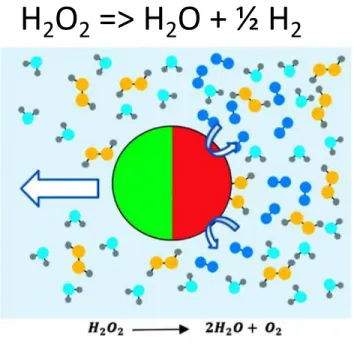
•  Conversion of chemical energy into motion due to decomposition of hydrogen peroxide (H ₂ O ₂ ) in a redox reaction

•  asymmetric reaction leads to an asymmetric free charge density which generates an electric dipole

•  Coupling of the electric field with the charge density leads to an electrical body force

•  Fluid motion due to the electrical body force propels the nanorod

•  Self-propelled swimming speed: up to 100 body lengths per second

swimming direction

Principles of the Self-Propulsion Mechanism

21

•  Indirect modeling of chemical reaction:

boundary conditions

anode cathode

Define molar proton fluxes on the cathode and anode surface with opposite signs

Moran et al., Phys. Rev. E 81, 065302 (2010)

Theoretical Description of the Pt/Au Nanorod

22

•  advection-diffusion equation:

•  Poisson equation:

•  Stokes equation for an incompressible Newtonian fluid:

Moran et al., Phys. Rev. E 81, 065302 (2010)

Theoretical Description of the Pt/Au Nanorod

23

•  Assume constant net charge density in the electrical double layer surrounding the rod:

•  Introduction of a characteristic electric field caused by the flux and diffusivity of protons:

•  With these assumptions the electroviscous velocity scales as

(Debye-Hückel approximation)

(increases linearly with reaction flux j)

Source: Moran et al., Phys. Rev. E 81, 065302 (2010)

Scaling of the Swimming Speed

24

•  Velocity increases linearly with dimensionless flux as expected

•  Dependence of on estimated from experimental data

•  Experimentally determined velocities:

•  Independent measurements found a native surface potential of

•  good agreement with simulation data

Moran et al., Phys. Rev. E 81, 065302 (2010)

Simulation Results: Nanomotor Velocity

Catalyticly driven Janus Spheres

Howse, J. R., R. A. L. Jones, A. J. Ryan, T. Gough, R. Vafabakhsh, and R. Golestanian, “Self-motile colloidal particles: From directed propulsion to random walk,”

Phys. Rev. Lett. 99, 048102 (2007)

Theoretical description of a persisten random walk

• Different molecular interactions at the surface create a concentration gradient (vdWaals attarction, HS repulsion, hydrophobic/hydrophilic)

• Chemical reactions at a catalyst create a concentration gradient

012001-3 Sharifi-Mood, Koplik, and Maldarelli Phys. Fluids25, 012001 (2013)

a

Interaction thickness L Solute molecules

Reactant (A) Product (B)

inert face

A B

Catalyst surface

z

R

a

Interaction thickness L

α_cap

θ

(a) (b)

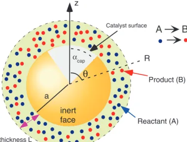
FIG. 1. Autonomous diffusiophoretic motion of a colloid particle: (a) unbalanced attractive intermolecular interactions between a colloid and a solute draw the particle to the side with higher solute concentration; (b) a reaction on a catalytic patch of the surface of a Janus colloid generates asymmetric concentration gradients of reactant (A) and product (B) solute molecules allowing the particle to propel itself.

solute for the catalyst is again the source of energy for the self-propulsion. Experimental studies of this mechanism^31,36,37 have once again used the platinum catalyzed reaction of hydrogen peroxide in aqueous solution to water and oxygen as the model surface reaction. Micron-sized, spherical

“Janus” particles, half-coated by thermal evaporation or sputtering with platinum and made of a nonconducting material (silica or polystyrene) to eliminate electrochemical processes, are placed in a hydrogen peroxide solution, and optical microscopy or fluorescence microscopy (using particles with an embedded fluorescent dye) was used to observe and track the motion. From the measured particle trajectories, velocities of the order of 1−10µm/S were calculated, but the movement was not rectilinear due to the Brownian rotation of the particles. Careful examinations of the orientation of the colloids as they are propelled^31,36,37 indicated that the particles moved with the catalyst surface at the back-end of the motion. If we consider the solutes to interact in an attractive interaction with the colloid (as a van der Waals attraction), then motion in the direction in which the reactant has a higher concentration implies that the attractive force of the reactant with the colloid is larger than the attractive force of the product, i.e., the propulsion arises from the net force of attraction. It is impor- tant to note however, that self-diffusiophoresis is not the only explanation for the observed motion as the expulsion of oxygen bubbles from the catalyst surface and the resultant colloid recoil can account for the directed movement. This motion, which is consistent with the observed orientation of the colloid with the catalyst at the back end, has been proposed and studied by Gibbs and Zhao,⁴² who in more recent work have designed colloids with different shapes and placement of the catalyst surface to improve the efficiency of the propulsion^43–46 interpreted in terms of the bubble ejection.

With the use of platinum catalyst, oxygen production on the catalyst surface is slow relative to the diffusion of oxygen from the particle. This acts to keep the oxygen concentration from exceeding the solubility limit, and thereby inhibits bubble production. And while macroscopic bubbles are not observed alongside the moving colloids, the ejection of microbubbles cannot be discarded.¹²Related studies by Schmidt and co-workers^47,48 used an immobilized enzyme catalyst with a much faster turnover rate for peroxide decomposition, which lead to observable bubble production. The design of their colloidal motor consisted of microtubules from rolled-up metallic sheets in which the enzyme catalyst is placed on the inside surface of microtubule cavity to funnel the oxygen propulsion for greater recoil.

The self-diffusiophoresis of colloids driven by solute gradients, which are sustained by a surface chemical reaction on one side of the colloid (Fig. 1(b)), merits attention as a possible mechanism of autonomous motion apart from the issue as to whether the observed motion of the platinum functionalized Janus colloids in a hydrogen peroxide solution is due to diffusiophoresis or the ejection of oxygen bubbles. The hydrodynamic theory of the reaction-driven, self-diffusiophoresis

N. Sharifi-Mood et al. Phys. Fluids, 25:012001, 2013.

Self-Phore*c Mo*on (due to Gradient Forces)

Fig. from R.J. Archer et al., Soft Matter11, 6872 (2015)

⃗" _# = −&'( _# + *( _# + _# ', _#

Repulsive Potential Attractive Potential -

Flux due to external Potential

Fick’s Law

MoJon induced by inter-molecular forces 0 _# = + _# ', _#

H ₂ O ₂ => H ₂ O + ½ H ₂

Origins of Self-Propulsion

The phoretic velocity, U

U = ⇠

^k _⌘

^T r _k C depends on the type of interaction.

Attractive potentials (e.g. van der Waals): the particle moves towards higher C .

Repulsive potentials (e.g. hard spheres, for which ⇠ = 0.5):

the particle moves towards lower C .

Based on: A. Brown and W. Poon. Soft Matter, 10:4016-4027, 2014.

Jorge Sauceda Di↵usiophoresis 06.05.2015 15 / 23

A. Brown and W. Poon. Soft Matter, 10:4016-4027, 2014.

The phoretic velocity, U

U = ⇠

^k _⌘

^T r _k C depends on the type of interaction.

Attractive potentials (e.g. van der Waals): the particle moves towards higher C .

Repulsive potentials (e.g. hard spheres, for which ⇠ = 0.5):

the particle moves towards lower C .

Based on: A. Brown and W. Poon. Soft Matter, 10:4016-4027, 2014.

Jorge Sauceda Di↵usiophoresis 06.05.2015 15 / 23

For attractive potentials (e.g. van der Waals) the particle moves towards higher C.

For repulsive potentials (e.g. hard spheres, for which x = -0.5) the particle moves towards lower C.

Solving the equations

Now we solve Stokes’ equation in the y direction:

⌘ @

v (y )

@z

@ p

(y )

@y = 0

⌘ @

v (y )

@ z

=



e

1 @ C (y )

@ y solving for v at a distance away from the surface:

v (y ) =

2

k

T

⌘

@C

@y

Z

0

s [e

1]ds where s is a point in the surface.

Jorge Sauceda Di↵usiophoresis 06.05.2015 13 / 23

Slip Layer Model

Particle based methods on atom scale: common in many areas, too many particles, reactions difficult to treat

Continuum equation based: neglect of molecular details, various levels of approximations

Hybrid methods (effective models, coarse-grained)

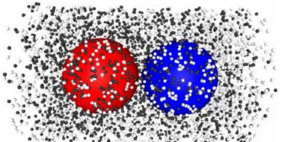
configuration in the vicinity of the nanodimer in the quasi- steady-state regime. The local density of species B varies from high to low along the nanodimer internuclear axis from the C to N spheres. The density field is asymmetric due to scattering by the noncatalytic sphere (see lower panel). In the absence of such a nonequilibrium gradient there is no directed motion. Since the reaction at the C sphere is irreversible, nanodimer directed motion will cease when all A species have been converted to B. In the curve labeled B in Fig. 2, all solvent molecules were of B type. Thus, no chemical reaction occurs, although the B particles still have different interaction potentials with the C and N nanodimer spheres. There is no net directed motion confirming that a nonequilibrium gradient is nec- essary for the effect.

Nanodimer dynamics is strongly influenced by fluctua- tions as seen in Fig. 4, which shows the probability distri- bution of V ! R ^ " V

. The mean nanodimer velocity is smaller than its standard deviation signalling the impor- tance of fluctuations for these small motors. The dimer will also tumble as it moves. The reorientational relaxation time, !

# 4#$R

=3k

T , is !

# 2000 for our nanodimer so that for %

" 5:0 the dimer will travel about 2–3 times its length before it reorients. Since !

scales as R

tumbling will be strongly suppressed for longer dimers.

We now consider the factors that contribute to the force on the fixed nanodimer. The coordinate origin is the cata- lytic sphere center with the dimer along the z axis. Thus,

R " R z ^ and the total z component of the force is

z ^ ! F " $ X

&"A

X

i"1

!

% z ^ ! r

& dV

% r

&

dr

'% z ^ ! r

& dV

% r

&

dr

"

: (2) Introducing the local microscopic density field for species

&, '

% r; r

& " P

i"1

( % r $ r

& , and its average over a

steady state or equilibrium distribution denoted by

'

% r & " h P

i"1

( % r $ r

&i , the average z component of

the force is

h z ^ ! F i " $ X

&"A

Z dr'

% r &% z ^ ! r ^ & dV

% r &

dr

$ X

&"A

Z dr

'

% r

' R &% z ^ ! r ^

& dV

% r

&

dr

: (3) The first and second integrals have their coordinate sys- tems centered on the catalytic C and noncatalytic N spheres, respectively.

To obtain the velocity we assume a steady state where the force due to the reaction is balanced by the frictional force: ) V

" h z ^ ! F i . Since the diffusion coefficient is related to the friction by D " k

T=) " 1=*) , we have

V

" D h z ^ ! *F i : (4)

The calculation hinges on knowing the nonequilibrium steady state densities. First, consider the forms of the equilibrium densities. Since there are no solvent-solvent forces the equilibrium density of A is given by

'

% r

& " n

e

; (5) where n

" N

=V is the density of A. A similar expression can be written for the B density. It is easy to see that if this expression is substituted into Eq. (3), the result is zero in view of the central forms of the LJ potentials. There is no directed motion in equilibrium.

To estimate the nonequilibrium density we make use of the solution of the diffusion equation

@n

% r; t &

@t " D

r

n

% r; t & ; (6)

with a radiation boundary condition (BC) at the catalytic sphere, ignoring, for simplicity, the presence of the non- catalytic sphere. Assuming that the BC is applied outside a boundary layer lying in the range +

* r * R

, the radia-

FIG. 3 (color online). Snapshot of the A (gray) and B (black) particles in the vicinity of the nanodimer in the quasi-steady- state regime. (lower panel) The average B density in a cylindrical shell versus z along the dimer bond.

-0.05 -0.025 0 0.025 0.05 V_z

0 5 10 15 20 25

p(V z)

FIG. 4 (color online). Probability distribution function p % V

&

of the center of mass velocity projected along the internuclear axis for %

" 5:0. The solid curve is a fit to a Boltzmann distribution with mean velocity V

" $ 0:0048.

PRL 98, 150603 (2007) P H Y S I C A L R E V I E W L E T T E R S

13 APRIL 2007

150603-3

G. Rückner, R. Kapral. Phys. Rev. Lett., 98:150603, 2007.

Modelling Approaches

Dissipative Particle Dynamics (DPD)

29

Brief introduction into Lattice-Boltzmann 12/23

Particle distribution function

Discretisation of time and drive towards local equilibrium

Full discretisation of time, space and velocities

f  x ,  p ,t  d

dt f =∇

f ⋅˙ x ∇

f ⋅˙ p ∂

f =∇

f ⋅ p

m ∇

f ⋅ F ∂

f

f  x ,t  t = f  x , t  1

⋅[ f

 x − f  x ,t ]

D3Q19 lattice

BGK or MRT collision rules Navier-Stokes Equation

recovered for long time scales

Boltzmann equation for kinetic theory of gases

The La'ce-Boltzmann Method

n Frictional coupling of MD particles to Lattice Boltzmann fluid [1]

n Modified Langevin equation:

n Momentum exchange between immersed particles and fluid

n Total momentum conservation

Hydrodynamic interactions

[1] P. Ahlrichs and B. Dünweg. International Journal of Modern Physics C, 9:1429-1438, 1998.

Current D3Q19 MRT Version with correct thermal fluctuation spectrum due to Schiller, Dünweg implemented in ESPResSo (www.espressomd.org)

Particle Coupling to LB

• Particle as velocity bounce-back boundary

• Bounce-back force on particle

• Delete fluid (LB populations) in front of particle when cell is claimed

• Create fluid behind particle when cell is vacated by averaging populations from neighbors

• Ladd, J. Fluid Mech. 271, 285 (1994)

• Aidun et al., J. Fluid Mech., 373, 287 (1998)

3 1

Moving Boundary LB

The yellow par,cle has a velocity v, whereas the dark par,cle is at rest.

a) When the yellow par,cle moves towards the darker one, it induces a repulsive force F12 on the darker par,cle due to the bow waves

b) when the darker par,cle is behind the yellow one, then the induced force F12 is a@rac,ve since the stern waves follow the brighter par,cles thus pulling the darker par,cle behind

Hydrodynamic Coupling of Two Colloids in a Fluid

Influence of Hydrodynamic Interactions on

Sedimentation

Poiseuille Flow in a Cylindrical Pipe

Turbulent fluid flow around an Obstacle

Ink in front of an Obstacle

Particles Coupled to Fluid Flow

2.3 Hydrodynamic interactions 15

v

!

v

!

F

T

v

!

"

"

"

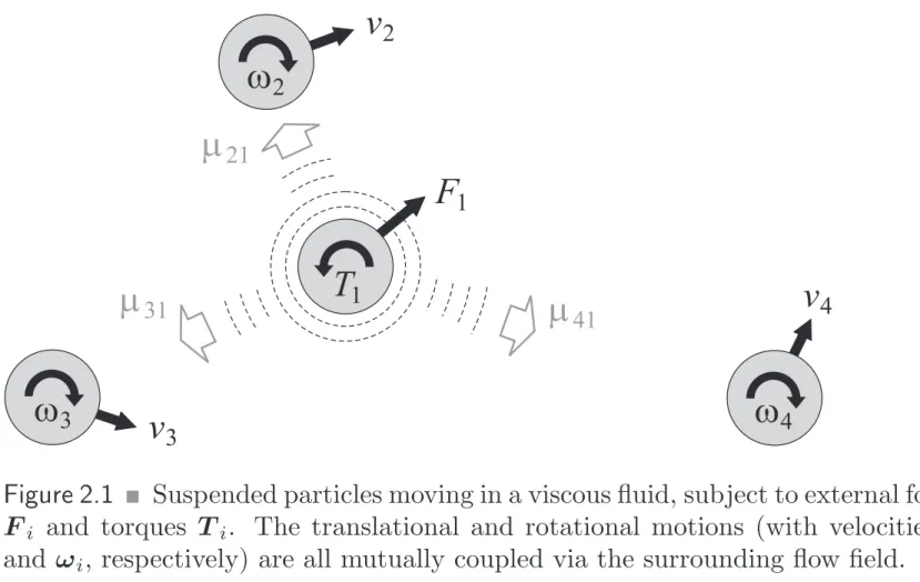
Figure 2.1

Suspended particles moving in a viscous fluid, subject to external forces F

and torques T

. The translational and rotational motions (with velocities v

and ω

, respectively) are all mutually coupled via the surrounding flow field.

Using Eq. (2.5), the torque needed to drive the particle at constant rotational speed ω is given by

T = − T

= ζ

ω (2.19)

with

ζ

= 1

µ

= 8πη a

. (2.20)

2.3 Hydrodynamic interactions

Particles moving in a viscous fluid create a flow field around themselves through which their motions are mutually coupled (Fig. 2.1). Hence, these so-called hy- drodynamic interactions constitute a complex many-body problem. The results of the previous section show that the perturbations of the fluid due to translations and rotations of suspended particles are of long range and so are the resulting interactions between the particles.

2.3.1 Theoretical description and definitions

We consider the motion of N colloidal particles suspended in an unbounded and otherwise quiescent viscous fluid at low Reynolds number. Furthermore, we neglect inertial effects, i.e., we are interested in time scales larger than the mo- mentum relaxation time (see discussion in Sect. 2.1.4). Thus, the interactions can

5

Comparing the asymptotic behavior of the respective flow fields (2.15) and (2.18), we see that rotational perturbations of the fluid decay faster ( | u(r) | ∝ 1/r

) than translational ones ( | u(r) | ∝ 1/r for r ≫ a).

REFERENCES A-1

References

[1] M. Reichert: Hydrodynamic Interactions in Colloidal and Biological Systems, Dissertation Universit¨at Konstanz, 2006

[2] J. Dhont: An Introduction to Dynamics of Colloids, Elsevier, Amsterdam, 1996

[3] J.H.C. Luke, SIAM J. Appl. Math., 49, 1635 (1989)

[4] H.C. ¨Ottinger: Stochastic Processes in Polymeric Fluids, Springer, Berlin, 1996

[5] Prof. Dr. Gerald Kneller: http://www2.fz-juelich.de, opened on 1 June 2012

Exp. vs Sim

• Velocity expanded in Legendre polynomials:

!

θ, % = '

(

)

% 2sin θ . . + 1

12

cos θ 1cos θ

• Velocity of center of mass:

!

= 2 3 )

• Dipole strength:

β = )

)

• Surface velocity:

:

= <

, > = 3

2 !

1 + β > ⋅ < =

> ⋅ < =

= <

− >

Lighthill 1952, Blake 1971 and Ishikawa et al., 2009

The Squirmer Model

• Use a slip model to efficiently treat systems with large numbers of swimmers

• Grid cells inside colloid treated as velocity boundary with

! _" ⃗$ _" = & + ( × (⃗$ − ⃗$ _" )

• Claimed cells’ populations are deleted

• Vacated cells are refilled with equilibrium populations

Squirmer in LB using Moving Boundaries

Squirmer

Tracer

Squirmer-Tracer Scattering

LB Raspberry Swimmers

134106-2 de Graafet al. J. Chem. Phys.144, 134106 (2016)

HI and strikes a balance between the accurate simulation of shape-anisotropic particles and computational efficiency. The LB algorithm has been shown to efficiently simulate HI and is therefore considered ideally suited to this task. In particular, the simulations of Nash et al.⁴⁰ demonstrate that LB can readily simulate thousands of swimmers.

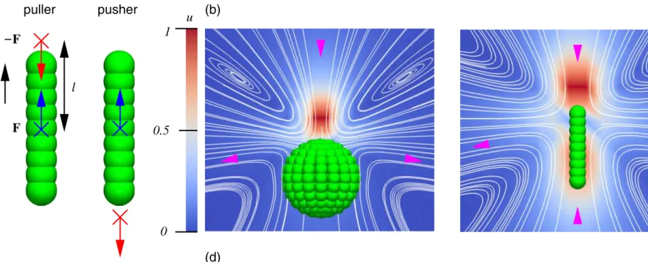
In this manuscript, we introduce a model with the aforementioned features. We simulate colloids of arbitrary shape by approximating them as clusters of spheres, see Fig.1.

These clusters are coupled to an LB fluid using the viscous coupling scheme introduced by Ahlrichs and Dünweg,⁶⁷ in which the friction depends on the relative velocity of particle and fluid. The e↵ect of this coupling is the formation of a hydrodynamic hull around the points, which thus gains an e↵ective hydrodynamic size.⁶⁷ Thereby, a solid particle can be modelled, which resembles a raspberry⁶⁸ for a sufficient density of coupling points.^69,70 Self-propulsion is introduced by following the principles of Refs. 39, 41, and 42: We

assign a direction (unit) vector to the raspberry particle and apply a persistent force along this direction and an equal and opposite (counter) force to the fluid, see Fig. 1(a). The location of the counter-force determines the nature of the leading dipole moment and distinguishes pusher (extensile) from puller (contractile) swimmers.

Using our model, we demonstrate that the anisotropy of the particle induces higher order multipole moments, in addition to the dipole moment that we impose. These multipole moments account for the flow of fluid around the object. We introduce a method to determine the magnitude of these multipole moments by means of a Legendre- Fourier (LF) analysis—we limit ourselves to axisymmetric anisotropic swimmers here. This characterization technique is applicable beyond our raspberry swimmers and may be of use in establishing the hydrodynamic nature of complex swimmers, for which the flow field has only been determined numerically.^71–74 We confirm that we obtain the correct

FIG. 1. The construction of raspberry swimmers. (a) A sketch of the construction of pusher and puller raspberry swimmers, in this case rods. The viscous coupling leads to an e↵ective hydrodynamic radius, as indicated by the use of green spheres with a radius comparable to the e↵ective one (⇠0.5 ). A forceF (blue arrow) is applied to the central bead (blue cross) in the direction of the symmetry axis ˆu(black arrow). A counter-force F(red arrow) is applied to the fluid at a pointluˆ(red cross), withl the dipole length. Forl>0 the particle is a puller and forl<0 it is a pusher. ((c) and (d)) The flow field around puller raspberry swimmers. The normalized magnitude of the flow velocity in the lab frame is indicated by the coloring (red max|u(r)|=1, dark blue|u(r)|=0) in a plane through the symmetry axis that is parallel to one of the box faces; only a part of the box is shown. The location of the counter-force point is clearly visible as a red region. The white curves are stream lines to the flow field and the magenta arrow heads indicate the direction of flow. We show three of our models: (b) the rod, (c) the sphere, and (d) the cylinder.

Reuse of AIP Publishing content is subject to the terms: https://publishing.aip.org/authors/rights-and-permissions. Downloaded to IP: 129.69.120.103 On: Wed, 13 Jul 2016 10:04:11

134106-2 de Graafet al. J. Chem. Phys.144, 134106 (2016)

HI and strikes a balance between the accurate simulation of shape-anisotropic particles and computational efficiency. The LB algorithm has been shown to efficiently simulate HI and is therefore considered ideally suited to this task. In particular, the simulations of Nash et al.⁴⁰ demonstrate that LB can readily simulate thousands of swimmers.

In this manuscript, we introduce a model with the aforementioned features. We simulate colloids of arbitrary shape by approximating them as clusters of spheres, see Fig.1.

These clusters are coupled to an LB fluid using the viscous coupling scheme introduced by Ahlrichs and Dünweg,⁶⁷ in which the friction depends on the relative velocity of particle and fluid. The e↵ect of this coupling is the formation of a hydrodynamic hull around the points, which thus gains an e↵ective hydrodynamic size.⁶⁷ Thereby, a solid particle can be modelled, which resembles a raspberry⁶⁸ for a sufficient density of coupling points.^69,70 Self-propulsion is introduced by following the principles of Refs. 39, 41, and 42: We

assign a direction (unit) vector to the raspberry particle and apply a persistent force along this direction and an equal and opposite (counter) force to the fluid, see Fig. 1(a). The location of the counter-force determines the nature of the leading dipole moment and distinguishes pusher (extensile) from puller (contractile) swimmers.

Using our model, we demonstrate that the anisotropy of the particle induces higher order multipole moments, in addition to the dipole moment that we impose. These multipole moments account for the flow of fluid around the object. We introduce a method to determine the magnitude of these multipole moments by means of a Legendre- Fourier (LF) analysis—we limit ourselves to axisymmetric anisotropic swimmers here. This characterization technique is applicable beyond our raspberry swimmers and may be of use in establishing the hydrodynamic nature of complex swimmers, for which the flow field has only been determined numerically.^71–74 We confirm that we obtain the correct

FIG. 1. The construction of raspberry swimmers. (a) A sketch of the construction of pusher and puller raspberry swimmers, in this case rods. The viscous coupling leads to an e↵ective hydrodynamic radius, as indicated by the use of green spheres with a radius comparable to the e↵ective one (⇠0.5 ). A forceF (blue arrow) is applied to the central bead (blue cross) in the direction of the symmetry axis ˆu(black arrow). A counter-force F(red arrow) is applied to the fluid at a pointluˆ(red cross), withl the dipole length. Forl>0 the particle is a puller and forl<0 it is a pusher. ((c) and (d)) The flow field around puller raspberry swimmers. The normalized magnitude of the flow velocity in the lab frame is indicated by the coloring (red max|u(r)|=1, dark blue|u(r)|=0) in a plane through the symmetry axis that is parallel to one of the box faces; only a part of the box is shown. The location of the counter-force point is clearly visible as a red region. The white curves are stream lines to the flow field and the magenta arrow heads indicate the direction of flow. We show three of our models: (b) the rod, (c) the sphere, and (d) the cylinder.

Reuse of AIP Publishing content is subject to the terms: https://publishing.aip.org/authors/rights-and-permissions. Downloaded to IP: 129.69.120.103 On: Wed, 13 Jul 2016 10:04:11

Swimming in Confinement

J. de Graaf et al., So- Ma/er 12, 4704 (2016)

Measuring Hydrodynamic Flow Fields

Particle Image Velocimetry requires finesse 48

K. Drescher et al., PNAS 108, 10940 (2011)

S. Jana et al., Phys. Fluids 24, 041901 (2012)

! ∝ 1/% ^&

! ∝ 1/% ^'

Hydrodynamic Mul/pole Expansion

Analogy to Electrostatics 49

K. Drescher et al., PNAS 108, 10940 (2011)

Oscillatory Trajectories in Confinement

Can we do something more with these trajectories? 50

S. Jana et al., Phys. Fluids 24, 041901 (2012)

L. Zhu et al., J. Fluid Mech. 726, 285 (2013)

Simple model System

51

J. de Graaf et al., Soft Matter 12, 4704 (2016) ⟹ "

ν

Summary

• Active matter: Particles that can convert energy into motion

• There are biological and synthetic counterparts

• Genuine out of equilibrium systems

• Modelling always on some coarse-grained level

• Hydrodynamic interactions are important

• Most modelling efforts in this seminar:

• Solving Continuum equations

• particle-LB coupling

• Langevin dynamics with driven particles