MINIBALL spectrometer

MINIBALL spectrometer

Inaugural-Dissertation zur

Erlangung des Doktorgrades

der Mathematisch-Naturwissenschaftlichen Fakultät der Universität zu Köln

Vorgelegt von David Pawel Rosiak

aus Solingen

Köln 2018

Prof. Dr. Jan Jolie

Tag der mündlichen Prüfung: 16. Juli 2018

Collective properties of the exotic doubly-magic nucleus

Sn, in particular the first excited 2

and 3

states, were investigated via safe Coulomb excitation. The experiment was performed in October 2016 at the HIE-ISOLDE facility at CERN. The challenging Coulomb excitation was realized utilizing the new commissioned stage 1 HIE-ISOLDE accelerator in combination with the high resolution and high efficient MINIBALL array. The radioactive

132

Sn beam was post accelerated up to 5.5 MeV/u and guided onto a 3.1 mg/cm

thick

206

Pb target. Projectile and target deexcitation were recorded in coincidence with the scattered nuclei to reduce the amount of background radiation in the γ -ray spectra and to perform the Doppler correction. B ( E 2), B ( E 3) and B ( E 1) values were determined for the corresponding transitions 0

→ 2

, 0

→ 3

, and 2

→ 3

of

Sn. The final reduced transition strengths are B ( E 2 ↑ ; 0

→ 2

) = 0 . 0869 ± 0 . 019 e

b

, B ( E 3 ↑ ; 0

→ 3

) = 0 . 11 ± 0 . 035 e

b

and B ( E 1 ↑ ; 2

→ 3

) = (9 . 05 ± 3 . 04) × 10

e

b. These experimental results were compared to state-of-the-art large-scale shell-model calculations, a relativistic random phase approximation and a random phase approximation calculation.

The second part of the present thesis deals with the manufacturing process and the first performance tests of the prototype escape-suppression-shield detector for the MINIBALL spectrometer. Measurements were performed with a stand-alone escape-suppression detec- tor and with the assembled system in combination with a MINIBALL triple cluster. The performance of the combined system was quantified via the peak-to-total ratio of measured

60

Co γ -ray spectra. A comparison between the achieved results of the prototype detection

system and prior performed Geant4 simulations is presented. The achieved peak-to-total

value of 41% with source measurements of the prototype detector is in good agreement

with the predicted value of 44%.

Die kollektiven Eigenschaften des exotischen doppelt magischen Kerns

Sn, insbesondere der ersten beiden angeregten Zustände 2

und 3

, wurden mit Hilfe von sicherer Coulomb Anregung untersucht. Das Experiment wurde im Oktober 2016 an der HIE-ISOLDE Ein- richtung am CERN durchgeführt. Der neu in Betrieb genommene HIE-ISOLDE Beschleu- niger (stage 1) in Kombination mit dem hochauflösenden und hocheffizienten MINIBALL Spektrometer ermöglichte die Durchführung des anspruchsvollen Experimentes. Damit konnte der radioaktive

Sn Strahl auf bis zu 5.5 MeV/u nachbeschleunigt und auf ein 3.1 mg/cm

dickes Target geleitet werden. Projektil- und Targetanregung wurden in Koin- zidenz mit den gestreuten Teilchen detektiert, um die γ -Quanten der Coulomb-Anregung zu selektieren und um eine Doppler-Korrektur der emittierten Photonen durchzuführen.

B ( E 2), B ( E 3) und B ( E 1) Werte wurden für die entsprechenden Übergänge 0

→ 2

, 0

→ 3

, und 2

→ 3

in

Sn bestimmt. Die reduzierten Übergangsstärken sind B ( E 2 ↑ ; 0

→ 2

) = 0 . 0869 ± 0 . 019 e

b

, B ( E 3 ↑ ; 0

→ 3

) = 0 . 11 ± 0 . 035 e

b

und B ( E 1 ↑ ; 2

→ 3

) = (9 . 05 ± 3 . 04) × 10

e

b. Die experimentell bestimmten Wer- te wurde mit modernen Schallenmodelrechnungen, einer relativistischen Random-Phase- Approximation und einer Random-Phase-Approximation verglichen.

Der zweite Teil der vorligenden Arbeit beschreibt die Fertigung und die ersten Performance-

Messungen des ”Escape-Suppression Shields“ (ESS) für das MINIBALL Spektrometer. Da-

für wurde der ESS als auch die Kombination aus ESS und MINIBALL-Cluster-Detektor

in der endgültigen Konfiguration vermessen und charakterisiert. Die Leistungsfähigkeit des

kombinierten Systems wurde anhand des Peak-zu-Untergrund Verhältnisses von

Co Spek-

tren quantifiziert. Die erzielten Resultate wurden mit zuvor durchgeführten Geant4 Si-

mulationen verglichen. Der mit dem Prototypen-Detektor gemessene Peak-zu-Untergrund

Wert von 41% ist in guter Übereinstimmung mit dem vorhergesagten Wert von 44%.

I. Coulomb excitation of doubly-magic

Sn 9

1. Nuclear structure and spectroscopic observables 11

1.1. Magic numbers . . . . 11

1.2. Nuclear shell model . . . . 14

1.3. Experimental observables . . . . 17

1.3.1. Binding energies . . . . 17

1.3.2. Proton and neutron separation energies . . . . 17

1.3.3. Electric quadrupole moment . . . . 17

1.3.4. Transition strength . . . . 20

1.4. Coulomb excitation . . . . 22

2. Physics case 32 2.1. Properties of Z = 50 and N = 82 nuclei . . . . 32

2.2. Previous Coulomb excitation of

Sn . . . . 39

3. Radioactive-beam physics at ISOLDE, CERN 41 3.1. The HIE-ISOLDE facility . . . . 43

3.1.1. Radioactive-ion beam production . . . . 45

3.1.2. Ion sources . . . . 46

3.1.3. Mass separators . . . . 48

3.1.4. Post accelerator . . . . 50

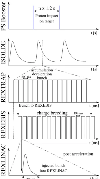
3.1.5. Beam time structure . . . . 58

3.1.6. MINIBALL setup . . . . 59

4. Experimental details of experiment IS551 64 5. Data analysis 65 5.1. Data acquisition and pre-processing . . . . 65

5.2. Detector calibration . . . . 66

5.2.1. DSSSD segment identification . . . . 66

5.2.2. DSSSD energy calibration . . . . 67

5.2.3. Energy calibration of MINIBALL . . . . 76

5.2.4. Efficiency calibration of MINIBALL . . . . 79

5.3. Doppler correction . . . . 80

5.4. Kinematic conditions . . . . 87

5.5. Particle- γ coincidence . . . . 89

5.6. Beam composition . . . . 91

6. Results 104 6.0.1. Selection of projectile and target-like nuclei . . . 104

6.0.2. Yield calculation . . . 113

7. Comparison with theoretical results 119 7.1. Theoretical models . . . 119

7.1.1. Relativistic Quasiparticle-vibration coupling . . . 119

7.1.2. Hybrid configuration mixing model . . . 120

7.1.3. Shell-model calculation based on

Zr . . . 120

7.1.4. Monte Carlo shell-model calculation . . . 121

7.2. Comparison . . . 123

7.3. Summary and Outlook . . . 128

II. Development of escape-suppression shields for the MINI- BALL spectrometer 131 8. Introduction 133 9. Geant4 simulations 135 9.1. MINIBALL escape-suppression shield . . . 135

10.Escape-suppression shield prototype 138 10.1. Escape-suppression shield design . . . 138

10.1.1. BGO crystals . . . 138

10.1.2. BGO housing . . . 140

10.1.3. Photomultipliers for the escape-suppression shield . . . 141

10.1.4. Mechanics holding structure of ESS detectors . . . 143

10.2. Experimental setup . . . 145

10.2.1. BGO signal processing . . . 146

10.2.2. Electronics . . . 149

11.Performance measurements with the ESS prototype 151

11.1. Escape-suppression shield . . . 151

11.2. MINIBALL escape-suppression detector . . . 153

11.2.1. Coincidence mode . . . 153

11.2.2. Free run mode . . . 157

11.3. Summary and Outlook . . . 161

Bibliography 165

List of figures 183

List of tables 186

Acknowledgements

Erklärung zur Dissertation

Curriculum vitae

Coulomb excitation of doubly-magic ¹³² Sn

Even today, the nuclear force and nuclear interactions are not completely understood. For a better understanding of atomic nuclei and the nuclear force one approach is to study the properties of nuclei depending on their proton-neutron configuration, which is known as nuclear structure. Doubly-magic nuclei are lighthouses along the whole chart of nuclei.

Their basic properties like masses, binding energies and excited states are essential for a detailed understanding and theoretical description in a vast range of the nuclear chart.

The doubly-magic nucleus

Sn and its vicinity provide essential reference points for all theoretical approaches in order to improve their forecasting power for nuclei which are not yet accessible.

1.1. Magic numbers

One of the most important discoveries, during the pioneering studies of atomic nuclei

and their nuclear structure, was that nuclei with specific numbers of protons or neutrons

(semi-magic nuclei) or both (doubly-magic nuclei) exhibit remarkable properties, e.g. large

binding and excitation energies [1, 2]. At this time, no theory was available to explain the

origin of these phenomena. Thus, these configurations were called “magic numbers”. The

magic numbers are Z = 2 , 8 , 20 , 28 , 50 , 82 and N = 2 , 8 , 20 , 28 , 50 , 82 , 126. It was observed

that the trend of the separation energy for either protons or neutrons is generally smooth,

except at certain specific nucleon numbers [2]. This is illustrated in Figure 1 where the two-

neutron separation energy in MeV of O,Ca,Kr,Cd,Ce,Hf,Pt,Pb and U along their isotopic

chains is shown. The separation energy exhibits discrete jumps at isotopes with neutron

magic numbers; the same is observed for nuclei with proton magic numbers. Moreover, the

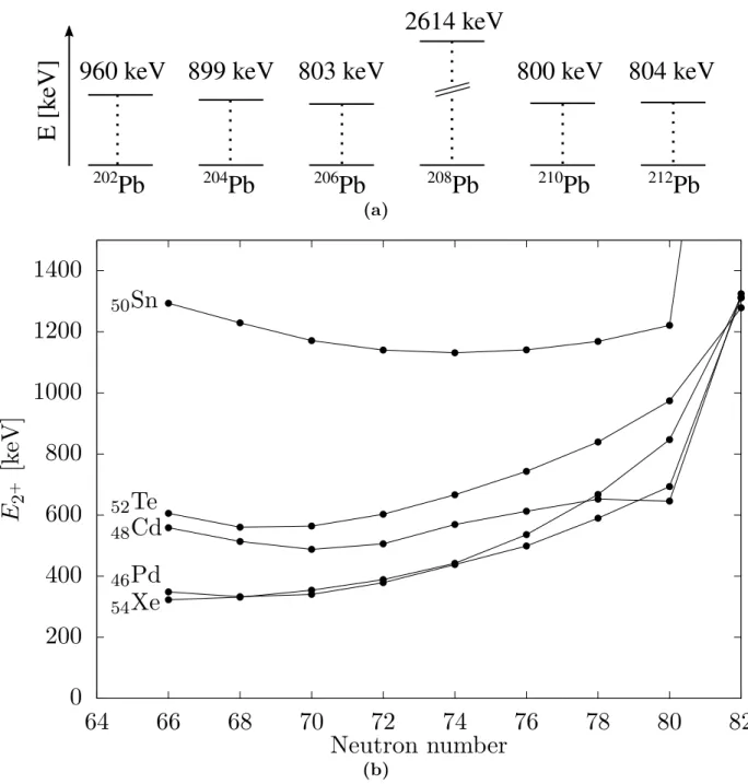
energy of the first excited state of nuclei with magic numbers is much higher compared to

their neighbors. This behavior is representatively shown, along the isotopic chain of lead,

in Fig. 2 (a). Figure 2 (b) illustrates this property along the isotopic chains of nuclei in

the vicinity of tin. The increased excitation energy for N = 82 is caused by the magic

configuration of neutrons in these nuclei. Furthermore, nuclei with configurations that

correspond to magic numbers have more stable isotopes and isotones compared to their

neighbors.

Figure 1: Two-neutron separation energy for isotopic chains including nuclei with magic

neutron configuration. At the classical magic numbers, sharp changes of the

tow-neutron energy can be observed. Otherwise the trend of the two-neutron

separation energy is smooth. Data taken from Ref. [3].

(a)

(b)

Figure 2: (a) Excitation energies for the first excited 2

state along the lead chain, including the doubly-magic

Pb. (b) First excited 2

state for isotopes of Sn, Te, Xe, Cd, Pd. For the Z = 50 shell closure (tin) the excitation energy is increased compared to the isotopes of the even-proton neighbors.

The excitation energy of the doubly-magic tin amounts to ∼ 4 MeV. Data

taken from Ref. [4].

1.2. Nuclear shell model

Atomic nuclei are many-body quantum systems, and can be partially compared to the electron cloud of an atom. The difference between this two systems, is the absence of a central potential inside a nucleus. Nevertheless, it is possible to treat protons and neutrons mathematically in a similar way, like it is done for the description of the electrons. For a nucleus with A interacting nucleons, the Hamiltonian can be written as a composition of kinetic energy and the interaction between all the nucleons. For protons also the Coulomb interactions has to be considered.

H =

i=1

T

+

i,j=1 i<j

V

(1.1)

In contrast to the electrons, the nucleon-nucleon interaction is not known from basic prin- ciples. However, binding-energy studies revealed that the nuclear interaction is predomi- nantly effective between two nucleons (two body interaction). This allows to describe the Hamiltonian of a nucleus with a nucleon-nucleon interaction V

:

H =

i=1

T

+

i,j=1 i<j

V

=

i=1

( T

+ V

) + (

i,j=1 i<j

V

−

A

X

i=1

V

) = H

+ H

, (1.2)

where V

is the mean field potential of the i th nucleon. For each nucleon the single-particle wave function φ

and the corresponding energy value

can be determined. A special solution for H

can be written as,

ψ =

i=1

φ

( ~ r

) . (1.3)

Protons and neutrons are fermions, thus they have to fulfill the Pauli-Principle. As a consequence, the complete solution of equation 1.2 has to be anti-symmetric. This can be achieved by the Slater-Determinant

ψ = √ 1

N ! Det |φ

( r ~

) | (1.4)

It can be shown that H

is the dominant contribution to the energy spectrum and H

is a small residual interaction [5]. In general H

can be interpreted as the description of A non-interacting single particles moving in an average potential produced by all A nucleons.

The residual interaction H

comprises the nucleon-nucleon interactions neglected by the simple approach of H

. For a theoretical treatment of the residual interaction see Ref. [5–

7]. Thus, this approximation fits better for nuclei with closed shells rather than mid- shell nuclei where many valence nucleons contribute to the final configuration. The first calculations for the mean-field potential were done with a harmonic oscillator potential and the Wood-Saxon potential. These approximations were able to predict first energy spectra and avoided the issue of the repulsive feature of the nuclear force. However, the predictions were not able to reproduce the phenomena of the discovered higher magic numbers. In 1949 Haxel, Jensen, Suess [1], and independently Maria Goeppert-Mayer [2, 8], proposed a strong spin-orbit coupling as an additional term for the nucleon-nucleon interaction, as it is done for the electrons in an atom.

V

= V ( ~ r ) + V

( ~ r )( ~l · ~ s ) (1.5) Where V ( ~ r ) is the central potential, V

( ~ r ) is a radial potential, which is basically the am- plitude of the spin-orbit coupling ( ~l· ~ s ) with ~l the angular momentum and ~ s the spin of the nucleon. This additional interaction enabled the theory to predict the nuclear magic num- bers “2,8,20,28,50,82,126” and in addition other properties (spins and magnetic moments) of many nuclei available at this time [1, 8]. Therefore, this theory was called ”nuclear shell model“. This modified nucleon-nucleon interaction induces an energy splitting for each state with total angular momentum j=l+s . Therein l is the orbital angular momentum and s is the spin, which can be parallel (+

) or anti-parallel ( −

) to the orbital angular momentum. Energy spectra for the three different potentials are shown in Figure 3. Only the first three magic numbers can be reproduced by the Wood-Saxon potential. The energy spectra for protons and neutrons with the spin-orbit coupling look almost identical, as long as the Coulomb interaction is not taken into account. However, recent experimental and theoretical findings indicate that magic numbers are not constant and valid for all nuclei.

For more exotic nuclei with high N/Z ratios new shell closures arise [10–13] indicating that

the configuration of spherical and more stable nuclei is related to the neutron-proton ratio.

Proton Neutron

126

82

50

28 20

8

2

Figure 3: Nucleon orbitals obtained via different shell-model calculations. (a) Harmonic

oscillator potential was used as the mean field. The resulting energy levels

are equidistant. (b) Wood-Saxon potential, which can describe the first three

magic numbers. (c) Strong spin-orbit coupling was implemented in addition

to the Wood-Saxon potential for the nucleon-nucleon interaction. Z indicate

the calculated orbits for protons and N for neutrons. This allows to reproduce

the magic numbers. See text for more details. Level configuration taken from

Ref. [9]

1.3. Experimental observables

The previous section indicated that there are still open questions in the understanding of nuclear structure, especially for exotic nuclei far from the so-called ”valley of stability“. The following sections focus on important observables that can be deduced from experiments and provide a better understanding of nuclear structure and nuclear force.

1.3.1. Binding energies

For the identification of shell and sub-shell closures primarily nuclear masses and binding energies are used. Figure 4 illustrates the difference between measured masses and results of the Bethe-Weizsäcker mass formula. The largest deviations are observed for the magic numbers, irrespective of the nucleon type. The reason is the increased binding energy for nuclei towards shell or sub-shell closures.

1.3.2. Proton and neutron separation energies

The two-nucleon separation energy is calculated from the binding energy S

= BE ( A, Z ) − BE ( A − 2 , Z ) and S

= BE ( A, Z ) − BE ( A − 2 , Z − 2). To compare the separation energy of neighboring nuclei the two-neutron and two-proton separation energy is considered, in order to neglect the effect of the pairing energy term in the Bethe-Weizsäcker formula.

As already seen in Figure 1, nuclei with magic numbers show larger separation energies compared to their next neighbor nuclei. The drop of the two-proton/neutron separation energy and the high excitation energies of the first excited states for magic numbers can be explained by shell closures of these nuclei (see Figure 3 (c)). Separation energies provide crucial information about the location of shell and sub-shell closures along the chart of nuclei.

1.3.3. Electric quadrupole moment

The nuclear shell model yields best results for nuclei with nearly or completely filled shells.

Nucleons of closed shells occupy all possible magnetic sub-states and lead to a spherical

density distribution of the nucleus. The nuclear electrical quadrupole moment Q is sensitive

to the charge distribution of the nuclear state. Therefore, Q vanishes for nuclei with magic

numbers and the absolute value increases towards mid-shell nuclei. Further information

can be deduced from the sign of the electrical quadrupole moment. Q < 0 corresponds to

a oblate shape of the nuclei, in a simple model it is related to particles outside of closed

(a)

(b)

Figure 4: Mass difference between experimental measured (M

) and calculated masses

with the Bethe-Weizacker formula (M

), for all measured isotones and iso-

topes. The largest deviations occur at magic numbers, due to the high binding

energies at closed shells. Experimental values taken from Ref. [3].

shells. Q > 0 corresponds to prolate shaped nuclei, induced by holes of fully filled shells.

Thus, Q is the quantum mechanical representation of the nuclear charge distribution, including the nuclear spin I and the projection of I onto the z-direction. This description of the nuclear deformation is illustrated in Figure 5. The quantity

is a measure for the nuclear deformation independent of the size of a nucleus. At all magic numbers the electric quadrupole moment reduce to zero and the deformation changes from prolate to oblate shaped nuclei. This behavior agrees with the aforementioned simple particle picture for the deformation. Therein, additional particles or holes in closed nuclei are related to the origin of nuclei deformation. In Figure 5 additional zero crossing points, besides the magic numbers, with Q > 0 to Q < 0 can be observed.

Q ZR

Figure 5: Quadrupole deformation of nuclei. The quantity

ZR²

is a size independent measure for the deformation of the nuclei with respect to a spherical nuclei.

The deformations are shown for different nuclei with odd number of protons or odd number of neutrons. Magic numbers are illustrated by dashed lines.

At the magic numbers the deformation get zero and a change from prolate to oblate shape is observed. This behavior is an indication for fully closed shells and, therefore, for magic numbers. Data taken from Ref. [14].

As mentioned before, new shell closures arise for nuclei far from stability. This was observed

for neutron-rich nitrogen, oxygen and fluorine nuclei with N = 16 [15, 16]. Nuclei with

forty protons or neutrons, also show properties of a shell closure [17]; however, forty is not

a classical magic number.

1.3.4. Transition strength

In section 1.1, energies of first excited states in nuclei demonstrated a clear increase at magic numbers. In addition to excitation energies also transition strengths of the electromagnetic radiation between nuclear states yield useful information about the underlying nuclear structure [18, 19]. Both quantities, excitation energy E ( I

) and reduced transition strength B( σλ ; I

→ I

), provide a signature for nuclear collectivity in even-even nuclei [9, 20].

The variables I

and I

denote the total angular momentum of the initial and final state of the nucleus, respectively. The character of the electromagnetic transition is represented by σ and can be electric E or magnetic M. The angular momentum carried by the emitted ra- diation is described by λ . The parity of electric multipole transition E λ is given by ( − 1)

and for magnetic multipole transition M λ the parity is determined by ( − 1)

. There- fore, even electric multipole transitions conserve the parity, whereas odd electric multipole transitions change the parity. For magnetic multipole transitions it is vice versa. Most low-lying nuclear states decay via electromagnetic processes i.e. γ -ray emission. These transitions can be described by reduced matrix elements h Ψ

| |M ( σλ ) | | Ψ

i , which provide information on the wavefunction of the inital and finale states [18, 19, 21]. Reduced matrix elements are identical for exciting and deexciting transitions with the same electromagnetic multipole operator M ( σλ ). The reduced transition probabilities are given by

B ( σλ, I

→ I

) = 1 2 I

+ 1

h Ψ

| |M ( σλ ) | | Ψ

i

(1.6) with Ψ

and Ψ

the initial and final state of the transition, respectively [9]. Reduced transition strengths for excitation and de-excitation, for the same set of states, are related by

B ( σλ, I

→ I

) = 2 I

+ 1

2 I

+ 1 B ( σλ, I

→ I

) . (1.7)

The reduced transition strength for electric multipole character is typically given in units

of e

b

and for magnetic multipole transitions µ

b

units are used. Thus, e denotes the

electric charge and µ

the nuclear magneton. Complementary to the ”direct“ measurement

of the transition strength via e.g. Coulomb excitation [22], it is possible to measure the

lifetime τ of an excited state. From the lifetime it is possible to determine the reduced

transition strength. The partial γ -decay rate of the emission of a γ ray of multipole λ ,

from the initial state I

into the final state I

can be calculated with

T ( σλ ; I

→ I

) = 8 π ( λ + 1) λ ~[(2 λ + 1)!!]

E

~ c

!2λ+1

× B ( σλ ; I

→ I

) . (1.8) If the decay, of the initial state into several final states is possible, these states have to be taken into account. Furthermore, the decay could also proceed via electron conversion.

Therefore, the conversion coefficient α ( λ ) has to be considered as well. Thus, the lifetime of the state I

can be described by:

τ ( I

) =



 X

I_f

X

λ

T ( σλ ; I

→ I

)[1 + α ( λ )]





−1

(1.9)

If only one final state and one multipole transition is possible, the reduced transition strength can be determined from the lifetime. For almost all even-even nuclei the first excited state is a 2

state and, therefore, a γ -ray decay only via a E2 transition into the 0

ground state is possible. In this special case the reduced transition strength can be written as:

B ( E 2; 2

→ 0

) = 8 . 16 × 10

[1 + α ( E 2)] E

τ (2+) . (1.10) The number of nucleons which contribute to an excitation of the nucleus can be roughly estimated with the so called Weisskopf units (W.u.) [9]. Therefore, the B ( Eλ ) and B ( M λ ) values are reevaluated in the following way:

B ( Eλ ; I

→ I

)

= 1 . 2

4 π

3 λ + 3

!2

A

, (1.11)

B ( M λ ; I

→ I

)

= 1 . 2

10 π

3 λ + 3

!2

A

. (1.12)

Equation 1.11 is expressed in e

fm

, whereas equation 1.12 in µ

fm

units. Weisskopf

units are used for single-particle transitions, where it is assumed that only one nucleon in

an average potential changes its orbit and contributes to the excitation. This is called the

0 20 40 60 80 100 120 140 160 180 200 220 240

0 20 40 60 80 100 120 140 160 180 200 220 240 260

B ( E 2;0

→ 2

) B ( E 2;0

→ 2

)

A

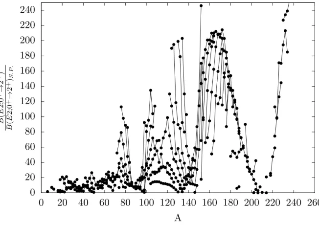
Figure 6: The reduced transition strength in Weisskopf units for 2

→ 0

transitions for all even-even nuclei. Nuclei with equal Z are connected by lines. The highest values are reached in mid-shell nuclei, whereas values around 1 are observed in closed-shell nuclei. This behavior can be explained by the high collectivity of mid-shell nuclei and the single-particle excitation of closed-shell nuclei. Data taken from Ref. [4].

single-particle picture [20]. A reduced transition strength of B ( E 2) ∼ 1 W.u. corresponds to a single-particle transitions, whereas higher values are expected for collective transitions with multiple nucleons contribute to the excitation. In Figure 6 the reduced transition strength is plotted in Weisskopf units. Peak maxima correspond to mid-shell nuclei and, hence, to collective excitation. The smallest values can be observed at magic numbers or closed-shell nuclei, where single-particle excitation is expected to dominate.

1.4. Coulomb excitation

Since the introduction of the Coulomb-excitation technique during the 1950s [18], this

method provided outstanding insight into e.g. collective properties of nuclei. In particular,

Coulomb excitation allowed to deduce a major part of the currently known transition probabilities and deformation parameters of atomic nuclei. Especially for exotic radioactive isotopes far from stability, Coulomb excitation provides a tool to access to B ( σλ ) values and potentially quadrupole moments, which are difficult to obtain via inelastic scattering and direct lifetime measurements.

*

*

Figure 7: Schematical illustration of a Coulomb scattering event in the center-of-mass system. At the point of closest ap- proach (d

) the interaction poten- tial V (~ r(t)) is strongest. After the in- elastic scattering, projectile and tar- get nuclei are excited indicated by as- terisks.

The goal of Coulomb excitation is to de- termine nuclear transition matrix elements by exciting atomic nuclei via pure electro- magnetic interaction. This implies, only the well understood electromagnetic in- teraction is contributing to the excitation and nuclear force effects can be neglected.

Therefore, a projectile nucleus with atomic

number Z

is guided onto a target nucleus

with atomic number Z

. If the energy of the

incident particle E

is below the Coulomb

barrier, the distance of closest approach

d

will be large enough to ensure no con-

tribution of the nuclear-force to the exci-

tation process. A schematical illustration

of this process is shown in Figure 7, in

the center-of-mass frame. It is immediately

clear that the excitation depends on E

, Z

,

Z

, the nuclei distance or the scattering an-

gle θ of the particles. The strongest inter-

action potential is reached at the point of closest approach and, hence, the excitation

probability is highest (see Fig. 7). To obtain the total excitation probability, the com-

plete particle trajectory has to be included in the calculation as the Coulomb force is a

long-range force. This boundary conditions and the well understood electromagnetic force

allow an accurate calculation of this processes involved i.e. the complex single and multiple

excitations. The theoretical procedure, which is used in Coulomb excitation calculation

codes e.g. GOSIA/GOSIA2 [23–25], was developed in the mid 50s and is presented in

detail in the paper of K. Alder et. al. [18]. In the following sections the basic concept will

be discussed.

Semiclassical approach

Apart of the quantum-mechanical approach in Ref. [18], Coulomb excitation can be treated in the semi-classical approximation, which presumes classical Rutherford trajectories along the whole scattering and excitation process. The electromagnetic excitation has a negligi- ble effect on the trajectories. Nevertheless, the excitation itself is treated fully quantum mechanically. This implies that the Coulomb-excitation cross section is a composition of the classical Rutherford scattering

and the quantum-mechanical probability for the excitation in which the particle was scattered into the solid angle d Ω. The quantum- mechanical probability P depends on the contributing nuclear states [19]. For a two-state model with initial level i and final level f the cross section is given by:

dσ d Ω

!

COU LEX

= dσ d Ω

!

RU T H

× P

. (1.13)

The classical Rutherford trajectories are preserved, if the size of the impinging projectile is much smaller than the size of the hyperbolic trajectory. This condition is expressed by the Sommerfeld parameter

η = d

2¯ λ

, (1.14)

where ¯ λ

is the de Broglie wavelength of the particle wave packet and d

/ 2 is half the distance of closest approach with

d

= Z

Z

e

E

= 2 Z

Z

e

mc

β

, (1.15)

where β =

is their impact velocity, m the reduced mass and Z

, Z

describe the proton number of projectile and target, respectively. The Sommerfeld parameter can be written as [9, 19]

η = Z

Z

e

~ ν = α Z

Z

β ≈ Z

Z

A

6 . 32 E

, (1.16)

with α = e

/ ~ c the unitless fine-structure constant and β =

2 E/mc

. For the present case

of Sn with a beam energy of 5.5 MeV/u impinging onto a Pb target, the Sommerfeld parameter equals η = 272. Hence, the semi-classical approach η 1 is applicable.

First-order perturbation theory

The excitation energy ∆ E also has impact on the excitation cross section. It is useful to define the adiabaticity parameter ξ , as the difference between incoming η

and outgoing η

,

ξ = η

− η

= Z

Z

A

∆ E

12 . 65 E

= η ∆ E

2 E

. (1.17)

For ξ ≤ 1 and small ∆ E a large excitation probability is expected, whereas for ξ 1 a vanishing excitation cross section will be the case, because high ∆ E hamper the Coulomb excitation [9]. Moreover, ξ can be interpreted as the ratio of the collision time relative to the time scale of internal motion of the nucleus.

ξ = τ

τ

(1.18)

If the collision time is much longer than the internal motion of the nucleus, the change of the electromagnetic field strength per time approaches the adiabatic limit and, hence no excitation is possible (adiabatic theorem) [26].

Considering the aforementioned semiclassical theory, excitation probabilities are deter- mined in time-dependent perturbation theory. Therefore, the condition of classical tra- jectories of the scattered particles has to be fulfilled. As equation 1.13 is valid for the projectile as well as for the target, both excitation probabilities and cross sections can be determined in an analog way by interchanging the corresponding properties of the calcu- lated nucleus. In perturbation theory the motion of the two particles is treated classically.

The time-dependent interaction potential V ( r ~ ( t )) originating from one collision partner influencing the second one, is used to calculate the excitation probability along the whole trajectory [21]. For unpolarized particles the probability P

from the state |iI

M

i to state |f I

M

i is expressed by

P

= 1 2 I

+ 1

X

M_iM_f

D

f I

M

b

iI

M

=

c

, (1.19)

with I

, M

and I

, M

, the spin and magnetic quantum number of the initial and final

state, respectively. The matrix elements b are given by

D

f I

M

b

iI

M

= 1 i ~

Z +∞

−∞

D

f I

M

V ( r ~ ( t ))

iI

M

e

dt, (1.20) with

= ω

. The excitation of the particles can be induced by either the electric V ( r ~ ( t ))

or the magnetic V ( r ( ~ t ))

component of the electromagnetic field. Thus, it is convenient to separate them. In the following the electric component is discussed and later on the magnetic contribution is reviewed. Performing a multipole expansion on the single components of the electric interaction potential the transition amplitude can be written as

D

f I

M

b

iI

M

= 4 πZ

e i ~

X

µλ

1 2 λ + 1

D

f I

M

M ( Eλ, µ )

iI

M

S

, (1.21)

where S

denotes the orbital integral along the classical trajectory r ~ ( t ):

S

=

−∞

e

Y

( r ~ ( t )) 1 r ~ ( t )

!λ+1

dt, (1.22)

with Y

( r ~ ( t )) the spherical harmonics [21]. The information about the nuclear structure is completely contained in the electric multipole matrix elements

D

f I

M

M ( Eλ, µ )

iI

M

, which can be defined as independent of the geometry of both nuclei by applying the Wigner-Eckart-Theorem:

D

iI

M

M ( Eλ, µ )

f I

M

= ( − 1)





I

λ I

−M

µ M





D

iI

|M ( Eλ, µ ) |

f I

. (1.23)

with the Clebsch-Gordan coefficient





I

λ I

−M

µ M





. The total transition probability is expressed as follows:

P

=

λ

P

( Eλ ) =

λ

4 πZ

e

~

!2

B(E λ ; I

→ I

) (2 λ + 1)

X

µ

S

, (1.24)

Figure 8: The integrated non-relativistic Coulomb-excitation function in dependency of the adiabaticity parameter ζ for electric multipole transitions with λ = 1, 2, 3, 4. Figure taken from [18] with kind permission from APS.

with the reduced transition strength B(E λ ; I

→ I

) defined in equation 1.6. The resulting differential cross section for a given electrical multipolarity λ is then described by

dσ d Ω

!

Eλ

= Z

e

~ ν

!2

d

2

!−2λ+2

B(E λ ; I

→ I

) f

( θ, ξ ) , (1.25) with the dimensionless non-relativistic Coulomb-excitation function f

( θ, ξ ) containing all information about the classical trajectory of the scattered particles. The dependency as a function of ξ is illustrated in Figure 8 for electric transitions up to λ = 4. For the magnetic part the excitation cross section is similar:

dσ d Ω

!

M λ

= Z

e

~ c

!2

d

2

!−2λ+2

B(M λ ; I

→ I

) f

( θ, ξ ) , (1.26)

From equation 1.25 and 1.26 can be deduced that a magnetic transition of the same mul- tipolarity is suppressed by a factor of β

= ( v

/c

), compared to a electric transition. At beam energies of 5.5 MeV/u for

Sn and a corresponding β ∼ 11%, electric transitions will dominate the Coulomb excitation process.

Second-order perturbation theory

In the framework of first-order perturbation theory, Coulomb-excitation probabilities are typically quite small P

1. However, for heavy-ion collisions the transition probabil- ity increases with the ion energy and, thus, the condition P

1 may not longer be satisfied and second-order effects have to be considered. This implies two consequences, i.e. first-order transition probabilities can be affected by second-order terms and states which were not accessible for example due to selection rules, can be populated via double excitation [27]. In this case the transition to the final state proceed via a multi-step ex- citation process. For multi-step excitation the probability increases with increasing beam energy [18, 19, 21]. To incorporate these effects, the perturbation of the nucleus by the changing electromagnetic field has to be considered up to higher orders, keeping the classi- cal trajectories. The transition probability for a multi-step excitation from the initial state i via an intermediate state m into the final state f is given by

P

=

c

+

m

c

2

=

c

+ 2 Re ( c

·

m

c

) +

X

m

c

2

, (1.27)

where c

is defined in equation 1.19 and

c

= 1 i ~

Z +∞

−∞

D

f I

M

V ( r ~ ( t ))

mI

M

e

× hmI

M

|V ( r ~ ( t )) |iI

M

i e

dt.

(1.28) From Equation 1.27 follows that the first-order and the second-order processes interfere [21].

Thus, it is important to include the second-order effects in the calculation, even for low

multi-step excitation probabilities. The interference between first-order and second-order

terms lead, e.g. to the reorientation effect. A typically occurrence of this effect is observed

by E2 absorption in even-even nuclei, where a transition from |mI

M

i to |f I

M

i with

m = f I

= I

can arise. Both state differ only in the magnetic sub-state of the same excited sate (usually 2

). In this case the matrix element

f I

M

M ( E 2)

mI

M

is proportional to the spectroscopic quadrupole moment

Q

=

v u u

t

16 πI (2 I − 1)

5( I + 1)(2 I + 1)(2 I + 3) × hI|M ( E 2) |I i . (1.29) For a spherical nucleus, e.g. the doubly-magic

Sn the quadrupole moment should be close to zero, as the quadrupole moment is a measure for the deformation of the nucleus.

With a precise determination of P

, the magnitude and the sign of Q

indicate the structure of the excited state.

Another consequence of second-order contribution is the two-step E2 excitation. In even- even nuclei the first 4

state can be excited either directly via an E4-transition or via a two-step excitation following the excitation scheme

0

− −→

2

− −→

4

. (1.30) Due to the much lower excitation probability of E4 compared to a E2 transition (cf. Fig. 8), the second-order contribution is essential. In almost all heavy-ion collisions the E4 first- order transition is superimposed by a much stronger excitation via the second-order two- step E2 transition. Both examples of the second-order perturbation theory are illustrated in Figure 9.

“Safe” Coulomb excitation

The so-called ”safe“ Coulomb excitation is characterized by a negligible effect of the nuclear force on the excitation of particles in a scattering experiment. The excitation of one or both scattering particles is induced by pure Coulomb interaction. A sufficient large distance between the two nuclear surfaces is necessary to satisfy this condition. The point of closest approach is restricted to

d

> R

+ R

+ ∆ D = 1 . 25( A

+ A

) + ∆ D, (1.31)

where R

, R

describes the nuclear radii of projectile and target, and ∆ D an addi-

tional “safe” distance.

Figure 9: Solid lines represent excitation, whereas dashed lines the de-excitation pro- cess. The schematic diagram show on the left side a one-step excitation from the initial level |ii to the final states |mi and |fi. On the right hand side the second-order processes are illustrated. The excitation to the final state |f i proceed via the intermediate state |mi. In addition, transitions within one state are possible, due to magnetic sub-state transitions. Further information in the text.

In reference [22] Cline et. al. determined an effect of less than 0.1% contribution of the nu- clear interaction in a Coulomb scattering experiment, with a safe distance of ∆ D = 5.0 fm.

Furthermore, the safe bombarding energy as a function of the scattering angle is calculated by

E ( θ

) = 0 . 72 Z

Z

d

A

+ A

A

1 + 1

sin

!

, (1.32)

with the scattering angle in the center-of-mass system θ

. Considering the conditions of the

Sn experiment, the point of closest approach for safe Coulomb excitation amounts to 18.75 fm. This would correspond to a safe bombarding energy of 3.9 MeV/u. To increase the Coulomb excitation cross section, an impinging energy of 5.5 MeV/u was chosen to facilitate the challenging experiment. However, for such beam energies the center- of-mass scattering angle has to be restricted to fulfill the safe Coulomb-excitation criterion.

The particle-scattering angles were restricted to 67 . 6

in the center-of-mass frame. This

corresponds to forward angles up to 42

with respect to the direction of the beam in the

laboratory frame.

Relative measurement of the transition strength

In Coulomb excitation experiments with insufficient knowledge of the beam current and its intensity, the Coulomb-excitation cross section can be determined relative to a well-studied transition. In the previous section it was explained that the number of scattered nuclei in a Coulomb-excitation experiment provides a direct measure for the excitation probability of the corresponding nuclei. This observable can be deduced from the measured γ -ray intensity after the de-excitation of the scattered particles.

N

( f → i ) =

b

σ

( f ) I ρd

N

A

(1.33)

The total number of detected γ -rays after an excitation of the projectile from an initial state |ii to the final state |f i followed by the deexcitation is determined by equation 1.33.

Therefore, the detection efficiency for the emitted γ -ray

, the branching ratio of the transition b

, the excitation cross section σ

( f ) for the final state, the beam intensity I and the number of scattering target nuclei ( ρd

N

) /A

has to be considered.

The number of target nuclei is expressed as the ratio of the product of target density times target thickness and the Avogadro constant divided by the atomic mass of the target nuclei.

The analog equation holds for the target excitation:

N

( f → i ) =

b

σ

( f ) I ρd

N

A

. (1.34)

From this follows that the ratio of the γ -ray intensities from projectile and target deex- citation is independent from the beam intensity. As the transition of the target nuclei is well known, all properties like branching ratios or excitation cross section are established with small errors. Thus the relevant excitation cross section can be written as

σ

( f ) = σ

( f ) N

N

b

b

. (1.35)

Using equations 1.25 and 1.26 the reduced transition strength can be determined with

the classical trajectories of the scattered particles and the corresponding solid angle. This

calculations are done with coupled-channel codes like CLX [28, 29] or GOSIA2 [23–25].

The physics motivation for the Coulomb-excitation experiment of the doubly-magic

Sn is described. In addition, previous results on a

Sn Coulomb-excitation experiment at HRIBF (Holifield Radioactive Ion Beam Facility) at ORNL are briefly discussed [30].

2.1. Properties of Z = 50 and N = 82 nuclei

More than 7000 nuclides are predicted to exist within the proton and neutron drip lines [31], until October 2016, nuclear ground-state properties for 3437 nuclei were observed in differ- ent experiments [32]. Astrophysical processes like the r-process (rapid neutron capture), which has a curcile role in the production of neutron-rich isotopes heavier than iron far from stability [33], proceed predominantly outside the area of known nuclei (cf. Figure 10).

N Z

126 82

50 20 28

82

50 28

8 20 8

r-process

_Sn

Figure 10: Nuclear chart with the magic numbers marked. The crossing points of magic proton and neutron numbers indicate the doubly-magic nuclei. Neutron-rich nuclei are marked in blue, neutron-deficient nuclei in red, stable nuclei in black and unknown nuclei in grey. One predicted r-process region is shown in blue. At N = 50, 82 and 126 the “waiting points” of the r-process are indicated. The r-process approaches very close to the doubly-magic

Sn.

132

Sn is the only neutron-rich doubly-magic nuclei above Z = 28 in the

region of the r-process predictions.

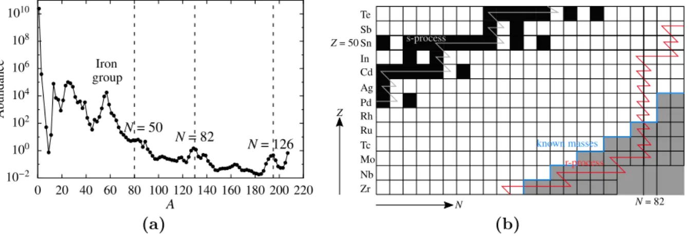
Thus, the origin and the exact progression of the r-process path are still unknown and remain an open question. The r-process proceeds along nuclei with constant neutron- separation energies to nuclei with increasing proton numbers, until the so called ”waiting points“ are reached. These ”waiting points“ correspond to nuclear-shell closures at N = 50, 82 and 126 [34], at which capture reactions and photodisintegration are in competition and further capture reactions to more neutron-rich nuclei get unlikely. Thus, the production of these nuclei are increased, and characteristic peaks in the mass abundance around A w 80, 130 and 195 are observed. The mass abundance in the solar system is illustrated in Figure 11 (a).

N = 50

N = 82

N = 126

A

(a)

N Z

known masses

N = 82 Z = 50

ZrNb Mo Tc RuRh Pd Ag CdIn SnSb Te

r-process s-process

(b)

Figure 11: (a) Nuclear abundance of the solar system. The characteristic peaks are produced by the r- and s-process of the nucleosynthesis. This increase in the abundance at A w 80, 130, 195 is related to the neutron shell closures at N = 50, 82 and 126. Data taken from Ref. [35]. Due to the increase of the neutron-separation energy and decrease of the neutron-capture cross section, the r-process proceeds along this so called “waiting points”, mainly via β-decay and neutron capture. (b) Theoretical r-process path (red) along the N = 82 magic number predicted in Ref. [36]. The white-grey path marks the s-process (slow-neutron capture) at the neutron-rich side of the valley of stability.

After reaching the “waiting points”, the weak interaction, in particular the β

-decay, drives the r-process along the chain of isotones up to nuclei with a magic proton configuration.

A theoretically predicted path of the described r-process around the shell closure N = 82

is shown in Figure 11 (b). For a detailed insight into this phenomenon, the knowledge of

nuclear properties, like the neutron-separation energy, the mass, the half-life ( T

) and the

neutron-capture cross section, especially at N = 50, 82, and 126 are mandatory in order to

perform r-process calculations, predictions and in order to improve the astrophysical un-

derstanding of the nucleosynthesis [37]. Therefore, extrapolations from theoretical models

(e.g. nuclear shell model), based on experimentally determined quantities of nuclei, are used to calculate the properties of unknown/unobserved nuclei. To perform extrapolations without exceeding the available computational power, closed-shell nuclei are essential, to accomplish the calculations for high nuclear masses. Including closed-shell nuclei in nuclear shell-model calculations, enables the investigation of nuclides in their vicinity by reducing the required model space. This limits the size of the Hamiltonian and the necessary compu- tational power. Hence, the properties of doubly-magic nuclei are of particular importance.

Out of the huge amount of today’s known nuclides, merely ten nuclei are observed that are classically doubly magic and, thus, exhibit fully filled proton and neutron shells (see section 1). Five of this nuclei i.e.

He,

O,

Ca,

Ca and

Pb are stable. The remain- ing five nuclei

Ni,

Ni,

Ni,

Sn and

Sn are radioactive. The properties of the stable doubly-magic nuclei are quite well studied [6]. For radioactive doubly-magic nuclei the situation is much more difficult, as the production of radioactive doubly-magic nuclei is challenging and in addition the experimental observation, too (see section 3). Nowadays,

132

Sn ( Z = 50 and N = 82) is the only observed doubly-magic nucleus above Z = 28 in the neutron-rich region far from stability and in immediate proximity to the r-process path. Thus, this nucleus is essential for efficient theoretical descriptions in this region.

The single-particle properties of this nucleus were already studied in the one particle/hole proton and neutron neighbors [38–41]. Besides single-particle properties, collective char- acteristics of nuclei are essential to develop and benchmark theoretical models e.g. nuclear shell-model interactions. The investigation of the collective properties of the doubly-magic

132

Sn nucleus, via Coulomb excitation, is presented in this work. In the following a brief summary of the experimentally determined characteristics of the shell closures at Z = 50 and N = 82 is given.

Figure 12: Shell-model orbitals forming the shell gaps at the magic numbers 50 and 82.

Shell closure along Z = 50

The nuclear shell gap at Z = 50 was investigated along the chain of tin isotopes, which includes the two doubly-magic nuclei

Sn and

Sn. This shell closure is created by fully filled orbitals up to the 0 g

orbital and the first empty orbitals 0 g

and 1 d

. Figure 12 illustrates the orbital configuration around the shell closures for Z = 50 and N = 82.

0 1 2 3 4

0 0.1 0.2 0.3

50 54 58 62 66 70 74 78 82

LSSM:

Energy(2+ 1)MeV

stable Sn isotopes

B(E2↑)[e2b2]

Neutron number

100Sn

90Zr

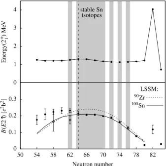
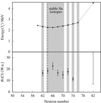
Figure 13: Top: Excitation energy of the first excited state 2

in even-even Sn nuclei along Z = 50. Bottom:

B(E 2 ↑) values along the isotopic Sn chain are illustrated. Data taken from Ref. [4]. Shell-model calcula- tions are from Ref. [42]. Values for

132

Sn were taken from Ref. [43].

In even-even tin nuclei the excitation en-

ergy of the first excited 2

state is nearly

constant between N = 52 and N = 84, ex-

cept for the magic number N = 82. The

upper plot of Figure 13 illustrates the mea-

sured excitation energies of the first excited

state along the Sn chain. The constant be-

havior of the excitation energies can be ex-

plained by the dense neutron-orbit distri-

bution between the shell gap N = 50 and

N = 82. The high density of states al-

lows for pairing correlations, which result in

similar excitation configurations [6]. Thus,

the 2

states around w 1 . 2 MeV are caused

by pure-neutron excitation. The small in-

crease of the excitation energy around N =

64 is an indication for a potential sub-shell

closure and a sub-shell gap between the

1 d

and 1 d

orbitals. At N = 82 the ex-

citation energy is increased, because the ex-

citation requires high energy for both, pro-

ton and neutron particles, to overcome the shell gap. Hence, the 2

state of the doubly-

magic

Sn is probably no longer of pure neutron character, it is rather a combination of

neutron and proton excitations. Further prove for the doubly-magic character of

Sn can

be deduced from the experimentally determined B ( E 2 ↑ ) value (preliminary value from

Ref. [43, 44]). In the bottom Figure 13, the B ( E 2 ↑ ) values for the even-even nuclei along

the isotopic tin chain are presented. For N > 64 the reduced transition strength follows

the parabolic trend of generalized seniority [45, 46], predicted by large-scale shell model

calculations [42]. For N < 64 a more constant behavior is apparent and, thus, indicate an