Broadband radio jet emission and variability of γ–ray Blazars
INAUGURAL-DISSERTATION
zur
Erlangung des Doktorgrades
der Mathematisch-Naturwissenschaftlichen Fakult¨at der Universit¨at zu K ¨oln
vorgelegt von
Ioannis Nestoras aus Larissa, Griechenland
K ¨oln 2015
Tag der letzten m ¨undlichen Pr ¨ufung: 22/06/2015
Abstract
AGN (Active Galactic Nuclei) and in particular their subclass blazars, are among the most energetic objects observed in the universe, featuring extreme phenomenological character- istics such as rapid broadband flux density and polarization variability, fast super–luminal motion, high degree of polarization and a broadband, double-humped spectral energy dis- tribution (SED). The details of the emission processes and violent variability of blazars are still poorly understood. Variability studies give important clues about the size, structure, physics and dynamics of the emitting region making AGN/blazar monitoring programs of uttermost importance in providing the necessary constraints for understanding the origin of energy production.
In this framework the F-GAMMA program was initiated, monitoring monthly 60 Fermi-GST detected AGN/blazars at 12 frequencies between 2.6 and 345 GHz since 2007.
For the thesis in hand observations and data analysis were performed within the realms of the F-GAMMA program, using the Effelsberg (EB) 100 m and Pico Veleta (PV) 30 m telescopes at 10 frequency bands ranging from 2.64 to 142 GHz. The cm to short-–mm variability/spectral characteristics are monitored for a sample of 59 sources for a period of five years enabling for the first time a detailed study of the observed flaring activity in both the light curve and spectral domains for such a large number of sources and such high cadence. Also the observing systems and methods are introduced as well as the data reduction techniques. The thesis at hand is structured as follows:
Chapter3presents the reduction methods and post measurement corrections applied to the data such as pointing offsets, gain–elevation and sensitivity corrections as well as specific corrections applied for each of the EB and PV observing systems respectively.
Chapter4presents the analysis tools and methods that were used such as: variability characteristics, flare amplitudes with a new method for estimating the intrinsic standard deviation, flare time scales using Structure Function analysis, spectral indices and spectral peak estimations.
Chapter5presents the results of the analysis performed upon the five year light curves.
The significance of variability through aχ2test is estimated as well as the flare amplitudes using the intrinsic variability of the light curves along with a new proposed k–index. The introduction of the k–index enables the characterization of the observed variability ampli- tudes across frequency, thus permitting us to limit the parameter space of various physical models. Also flare time scales, brightness temperatures and Doppler factors are reported.
Chapter6presents the corresponding analysis in the spectral domain, including results for spectral indices and an Smax–νmaxanalysis. By determining the spectral peak of every spectra for a selected number of sources, it is possible to track the evolution of the flaring activity in the Smax–νmaxplane, enabling us to discriminate between different underlying physical mechanisms that are in action. FinallyChapter7includes the overall discussion and a summary of results obtained.
Aktive Galaxienkerne (engl. AGN), insbesondere die Unterklasse der Blazare, z¨ahlen zu den energetischsten Objekten des beobachtbaren Universums. Sie zeigen extreme ph¨ano- menologische Charakteristika wie rapide Variation der Flussdichte und der Polarisation
¨uber den gesamten Spektralbereich, Bewegung mit scheinbarer ¨Uberlichtgeschwindigkeit, hohe Polarisation und eine spektrale Energieverteilung, die das gesamte Spektrum ab- deckt, mit einem typischem Verlauf , der zwei Maxima im niedrigen und hohen Energiebe- reich zeigt. Die Details der Emissionsprozesse und der drastischen Variabilit¨at sind bislang nicht vollst¨andig verstanden. Untersuchungen der Variabilit¨at geben Hinweise auf die Gr ¨oße, Struktur, Physik und Dynamik der strahlungsemittierenden Region. Daher sind kontinuierliche AGN/Blazar-Beobachtungskampagnen von h ¨ochster Bedeutung, um den Ursprung der Energieproduktion zu verstehen.
In diesem Rahmen wurde das F-GAMMA Programm initialisiert, in welchem seit 2007 monatlich etwa 60 von Fermi-GST identifizierte AGNs/Blazare in 12 Frequenzen zwis- chen 2.6 und 345 GHz beobachtet werden. F ¨ur diese Doktorarbeit wurden Beobachtun- gen am Effelsberg-100 m-Teleskop (EB) und am Pico Valeta-30 m-Teleskop (PV) in 10 Fre- quenzb¨andern von 2.64 bis 142 GHz durchgef ¨uhrt sowie die zugeh ¨orige Datenanalyse. Die Beobachtung von 59 Objekten in verschiedenen Frequenzen ¨uber einen Zeitraum von f ¨unf Jahren erlaubt zum ersten Mal das detaillierte Untersuchen von Intensit¨atsausbr ¨uchen (Flares) sowohl in den Lichtkurven als auch in den Spektren f ¨ur eine große Anzahl von Objekten bei so hoher Zeitaufl ¨osung. Die Beobachtungssysteme und -methoden werden in dieser Arbeit vorgestellt, ebenso wie die Methoden der Datenreduktion. Die Arbeit ist in nachfolgende Kapitel unterteilt.
In Kapitel3werden die Methoden der Datenreduktion vorgestellt, die nach der Beoba- chtung angewendeten Korrekturen, darunter Offsets der Teleskopausrichtung, Signalve- rst¨arkung, Sensitivit¨ats und spezifische weitere Korrekturen, die auf die Daten der EB und PV Systeme angewendet wurden.
In Kapitel4werden die Methoden der Datenanalyse dargestellt, darunter die Charak- terisierung der Variabilit¨at, der Flare–Amplituden mit einer neuen Methode zur Einsch¨at- zung der intrinsischen Standardabweichung, der typischen Flare–Zeitskalen mittels An- wendung der Strkturfunktion sowie Absch¨atzung der spektralen Indizes und der Maxima der spektralen Energieverteilung.
In Kapitel 5werden die Ergebnisse pr¨asentiert, die auf der Untersuchung der 5-Jahres- Lichtkurven basieren. Die Signifikanz der Variabilit¨at wird mittels einesχ2–Testes abgesch-
¨atzt sowie die Amplituden der Flares unter Verwendung der intrinsischen Variabilit¨at der Lichtkurven und dem hier neu eingef ¨uhrtem k–Index. Der k–Index erlaubt die Charak- terisierung der beobachteten Variabilit¨atsamplituden ¨uber den gesamten Frequenzbereich und erm ¨oglicht es somit Schranken f ¨ur die Parameter verschiedener physikalischer Mod- elle zu finden. Des Weiteren werden Flare-Zeitskalen, Strahlungstemperatur und Doppler- Faktoren diskutiert.
In Kapitel 6werden entsprechend die Ergebnisse der Spektralanalyse dargestellt, daru-
iii nter die Spektral-Indizes und die Smax– νmax Analyse. Indem das Maximum jeder spek- tralen Energiedichte verschiedener Objekte ermittelt wird, ist es m ¨oglich die Entwick- lung eines Intensit¨atsausbruches in der Smax–νmax Ebene zu verfolgen. Dies erlaubt ver- schiedene physikalische Prozesse zu unterscheiden, die Ursache f ¨ur dieses Verhalten sind.
In Kapitel 7werden die Ergebnisse dieser Doktorarbeit und deren Interpretation zusa- mmengefasst.
When I started writing the acknowledgements, I realized that the difference in choosing the proper words to express myself, from the somewhat proper words is similar to the difference between night and day. In that sense if I forgot someone or if someone feels not properly acknowledged please have in mind that I did my best to express my feelings and thoughts but certainly not succeeded completely.
First of all I would like to thank my family, my mother Elpiniki my brothers Alekos and Petros my uncle Petros and my grandmother Kiki. Without them I would not be the man I am now and certainly without their help I would not have been able to accomplish anything. The security I felt throughout the years being able to pursue my dreams, is something you can not buy, but only be given and only if you are lucky enough to be blessed with a family supporting you like mine. I don’t simply thank them but owe them everything. This thesis is devoted to all of them that are still here beside me and to those that have left from this life.
Secondly I would like to thank my friends, that stood beside me in good and bad mo- ments. Specifically I would like to thank my dear friends A. Tsitali and V. Karamanavis. I owe them a lot, without them I wouldn’t be able to finish this quest. Their help is far be- yond the simple and practical things and lies in true friendship that never dies or is forgot- ten. My dear friends I. Antoniadis, L. Tremou, I. Miserlis, K. Markakis, K. Papadopoulou, K. Metallinos, X. Milea, V. Oikonomou, K. Lazarides, H. Kalantarova, O. Vantzos, E. Kat- sikogiani and S. Lopez for being there when I needed them, I shall never forget the amaz- ing times we had together all those years. Living abroad without them would have been a torture. Also I could not have forgotten X. Spilioti for the long conversations by the Rhine and for her true friendship in bad times, I honestly thank her for that.
My gratitude to V. Papaioanou, it was an honour for me being my friend all those years, teaching me even until his last moments on how to truly live life and for playing a key role to experiences that can not easily be explained. Some memories are never forgotten and will always remain.
A special place in my heart has Prof. J. Seiradakis. Because of him I started my journey into astronomy, because of him I have so many more experiences that I wouldn’t be able to have in any other way. He was the beginning and thus I am infinitely grateful for all the knowledge and support he gave me in my humble beginnings.
Many people played a key role for the completion of the thesis in hand. I would like to thank my supervising professor Dr. A. Zensus, for the trust, resources, patience and overall support over the years. My advisor Dr. L. Fuhrmann, his guidance and comments all these years, in good and in bad times, played a key role to the success of this endeavour.
Special thanks goes to Dr. E. Angelakis for his help and support.
I truly thank Dr. V. Pavlidou, Dr. N. Marchili and Dr. T. Krichbaum for their significant help and contribution to several key scientific aspects of this work. Their contribution was of uttermost importance. I also thank all the people in the VLBI group for accepting me as one of their own. My office mates and colleagues Dr. F. Schinzel, Dr. M. Karouzos, Dr. M.
v
Mezcua and Dr. C. Fromm I thank them all for their friendship and patience with me. Also I would like to thank S. Kielhlmann for the quick translation of the abstract to the German language. Special thanks goes also to Kostas Markakis and Nadeen Sabha for their real help with the practicalities at the last moments. I can not forget also K. Gotzman for her help with all the trivial but important papers of the University. The secretaries of the MPI and IMPRS for their help all these years, Dr. Simone Pott and Beate Naunheim.
Also I would like to thank all the operators in both Effelsberg and Pico Veleta tele- scopes. All the countless nights and days of observing would have been far more difficult without their technical support and friendly company.
Last but not least, I would really like to thank all those that stood in my way trying to make my life difficult. Without them I could not have obtained the cast of mind and mental strength that is required to successfully accomplish anything in life. All of you, I thank you from the deepest part of my heart !!
“Words have no power to impress the mind without the exquisite horror of their reality”
Edgar Alan Poe
Contents
1 Introduction 1
1.1 Historical background . . . . 1
1.2 AGN structure . . . . 3
1.3 AGN Classification & Unification . . . . 4
1.4 Physical processes in Blazars . . . . 7
1.4.1 Relativistic beaming & Superluminal motion . . . . 7
1.4.2 Synchrotron emission & absorption . . . . 8
1.4.3 Inverse Compton Scattering: SSC & EC . . . . 10
1.5 Variability of Blazars . . . . 10
1.5.1 Shock–in–Jet model. . . . 10
1.5.2 Geometrical models . . . . 12
1.6 F-GAMMA Program description . . . . 13
1.7 Scope of current thesis . . . . 15
2 Observations 17 2.1 The Source sample . . . . 17
2.1.1 Redshift distribution of F-GAMMA Blazars . . . . 18
2.1.2 The Dataset . . . . 18
2.2 Observing methods . . . . 19
2.2.1 Observing modes . . . . 20
2.2.2 Switching Modes . . . . 22
2.2.3 Focus & Calibration . . . . 23
2.3 EB - PV cross calibration . . . . 24
2.4 Observing logistics . . . . 25
2.4.1 Time allocation . . . . 25
2.4.2 Coherence time and Sampling . . . . 26
3 Pico Veleta & Effelsberg data 29 3.1 The IRAM 30–m telescope . . . . 29
3.1.1 PV System Description . . . . 29
3.1.2 Data reduction . . . . 32
3.1.3 Post-measurement corrections . . . . 35
3.1.4 Error estimates . . . . 39
3.2 PV system studies . . . . 43
3.3 The Effelsberg 100–m telescope . . . . 47
3.3.1 System Description . . . . 47
3.3.2 The receivers . . . . 47
3.3.3 Data reduction and calibration . . . . 49
3.3.4 Post–measurement corrections . . . . 52
3.3.5 Error estimates . . . . 56
4 Analysis tools and methods 59 4.1 Significance of variability: theχ2–test . . . . 60
4.2 Intrinsic standard deviation . . . . 61
4.2.1 Gaussian flux distribution . . . . 63
4.2.2 Bi–modal flux distribution. . . . 64
4.3 Flare time scales . . . . 64
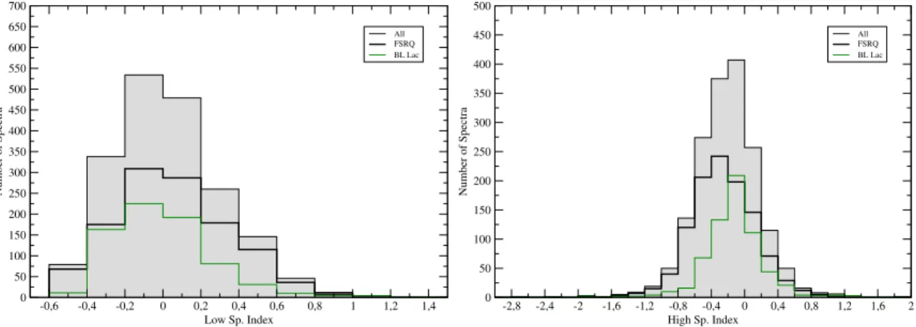
4.4 Spectral indices . . . . 66
4.5 Spectral peak analysis . . . . 67
5 Light Curve analysis 69 5.1 Observed light curves . . . . 69
5.2 Variability test . . . . 70
5.3 Variability amplitudes & k–index . . . . 72
5.4 Observed time scales . . . . 75
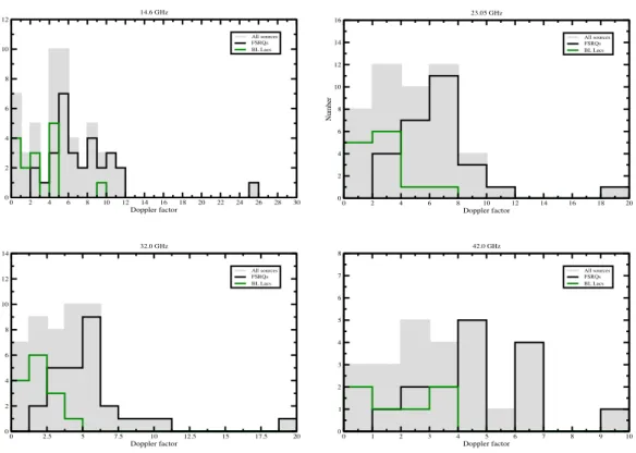
5.5 Brightness temperatures & Doppler factors . . . . 76
6 Spectral analysis 83 6.1 Observed spectra . . . . 83
6.2 Spectral indices . . . . 86
6.3 Smax–νmaxanalysis . . . . 89
6.3.1 Flare sample . . . . 89
7 Discussion and Summary 95 7.1 Discussion . . . . 95
7.2 Summary of Results. . . 100
7.3 Future work . . . 103
A Appendices 105 A.1 Data Tables. . . 105
A.2 Spectra . . . 113
A.2.1 Spectral plots . . . 113
A.2.2 Spectral indices plots . . . 124
A.3 Light Curves . . . 132
A.4 Smax–νmaxplots. . . 144
A.5 Kolmogorov–Smirnov Test . . . 148
CONTENTS ix
A.6 IDL Software description . . . 150
List of Figures 157
List of Tables 161
Bibliography 163
1
Introduction
With the opening of the radio window in the 60’s many great discoveries were made.
The discovery of the microwave background, pulsars and quasars are among the most important. The term “quasar” originally stood for “quasi–stellar radio source”, and refers to the fact that these type of objects are point like and appear very similar to stars when are observed in the optical. These sources belong to a class of objects called AGN, which stands for “Active Galactic Nuclei”. In the following a brief introduction to this type of objects and to their different observed flavours is given.
1.1 Historical background
In the beginning of the twentieth century,Fath(1909) made the first observations in order to clarify the nature of the “spiral nebulae”. The question back then was if these nebulae are similar to other well known objects as the Orion nebulae or a collection of unresolved stars.Seyfert(1943) began observations systematically of galaxies with emission lines. He obtained spectrograms of 6 galaxies with nearly stellar nuclei showing emission lines su- perimposed on a normal G-type star spectrum. These type of galaxies today are called Seyfert galaxies in honour of the work of Carl Seyfert. The next leap came with the de- velopment of radio astronomy in the 60’s. In 1963 the first quasars where discovered by Schmidt (1963) with the observations of 3C 273. These first results were also published in papers by Hazard et al.(1963);Schmidt(1963);Oke(1963);Greenstein and Matthews (1963) and their most reasonable explanation was that these objects were extragalactic in nature with redshifts that according to Hubble expansion where placing them far beyond our own galaxy. In particular 3C 48 was identified also in the optical as a variable source (Matthews and Sandage 1963), with strong emission lines in its spectrum. An example of
a quasar imaged in different wavelengths is shown in Fig.1.1.
Figure 1.1:A typical case of a quasar. Cen A at different wavelengths demonstrating the different morphologies observed in AGN.
Today we know that these objects exhibit a compact core at the center and extended radio structures and are the largest single known astronomical sources in the universe.
Their energy content is very large up to 1043erg/s. The origin of this energy and the way it is converted into relativistic particles and magnetic fields is one of the most challenging problems of modern astrophysics. Several properties of this new class of objects emerged:
• star like objects identified with radio sources
• time variable flux density
• large UV flux
• broad emission lines
• large redshifts
• compact nucleus and jet structures in the radio bands
Today these galaxies are part of what we call an AGN. So, at a basic level, AGN are simply the cores of galaxies that are in contrast to “normal galaxies” active. Not all AGN share all of the above properties.
One of the defining characteristics of quasars and AGN is their broad spectral energy distribution (SED). An example of an SED of the powerful blazar 3C 454.3 can be seen in Fig. 1.2. Typically AGN are among the brightest objects in the sky at every observable frequency. AGN spectra can not be described simply in terms of black body emission like in the case of stars. Non-thermal processes are needed to explain the observed shape of their spectra. The primary process is incoherent synchrotron radiation for the low SED bump (see Sect.1.4).
The radio morphology of AGN is described by extended structures that are resolved by modern imaging techniques. VLBI radio images show a very compact feature which is thought to be close to the “central engine” of the AGN producing the energy needed. The
production region a black hole fed by an accretion disk of falling material and launching relativistic jets alongside magnetic field lines. This AGN paradigm is graphically illus- trated in Fig.1.3. Broad emission lines are produced in clouds orbiting near the black hole.
A thick dusty torus obscures the broad-line region from transverse lines of sight. A hot corona above the accretion disk plays a role in producing the X-ray continuum. Narrow lines are produced in clouds farther away from the central engine. In summary the basic structure of an AGN includes:
• A black hole, acting as the central engine of the AGN, with a mass range of 106Mo
M 1010Mo.
• An accretion disk, matter with angular momentum, spirals into the black hole and forms a disk.
• An X–ray corona, surrounding the accretion disk. The X-ray emission is variable on short time scales implying a very compact region. Its luminosity is is linked to opti- cal/UV emission from the accretion disk.
• An obscuring torus, surrounding the black hole and accretion disk on parsec scales, absorbing some part of the radiation and re-emitting it in the infrared.
• Broad Line Region(BLR), a region of small fast moving clouds close to the black hole at a distance of 1017–1018cm and displaying spectral lines with large velocity widths.
They absorb 10% of radiation of the accretion disk, and re emit it in the form of lines.
• Narrow Line Region (NLR), similar to the BLR region but at larger distances of the order of 100 pc with less dense clouds that are moving with smaller speeds.
• Jets, about 10% of AGN exhibits two oppositely directed jets. The material inside the jets is moving at relativistic speeds causing relativistic effects. As it will be discussed later jets are the key ingredient for the range of phenomena observed.
1.3 AGN Classification & Unification
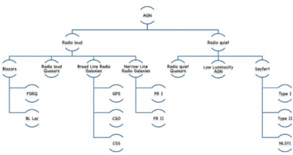
AGN exhibit a wide variety of different observational signatures. Some AGN produce powerful radio jets while others do not, some produce powerful X-ray andγ–ray emission as well as broad optical emission lines and are highly optical polarized and others are not, some are strongly variable while others are not. The main host galaxies of radio-quiet AGN seem to be spirals in contrast to powerful radio loud AGNs that are usually found only in ellipticals. Complicated at first glance a classification of all this phenomenology exists, as shown at Fig.1.4. The causes of these diverse characteristics can be traced down to the combination of the AGN structure and the angle of the jet towards earth i.e. the line of sight.
1.3 AGN Classification & Unification 5
Figure 1.4:Schematic view of the AGN classification with different types and sub-types according to our current understanding.
Two major sub-divisions exist, radio-loud and radio quiet AGN. The first quasars ever discovered were radio loud, but we now know that the majority is radio quiet and that radio loud AGN are only 10% of all AGN population. The separation in terms of radio loud and radio quiet is based on the flux density ratio at 5 GHz to optical flux in the B–
band, with radio loud AGN having ratios of Fradio Foptical 10 (Kellermann 1989). Radio loud AGN are further sub-divided into the classes of blazars, Broad Line Radio Galaxies (BLRG) and Narrow Line Radio Galaxies (NLRG). Radio-quiet AGN are sub-divided into radio quiet quasars, Low luminocity AGN (LLAGN) and Seyfert galaxies.
These classifications are based upon the observed characteristics that include spectral properties, structure at radio and other wavelengths. Blazars are furthermore divided into Flat Spectrum Radio Quasars (FSRQ) and BL Lac objects, NLRG are divided to FR I and II types, BLRG into GPS (GHz Peaked Sources), CSO (Compact Symmetric Objects) and CSS (Compact Steep Source) sources. Seyfert galaxies are further sub-divided into Type I and II and NLSY1 sources. The vast array of different phenomena and types can be unified under a relative simple model. This unified scheme is graphically demonstrated in Fig.1.5.
The main idea is that the type and thus the phenomena we observe from an AGN largely depend on the line of sight towards the observer. In principle all AGN have the same basic structure but their appearance changes with the angle that we look upon them. Below a brief explanation of the most important AGN sub-types is given :
• Blazars
An AGN is called a blazar in the case that the line of sight is aligned with the jet and thus the observer looks directly into the jet. This type of objects are the most variable and belong to the radio loud category of AGN. Relativistic boosting of the radiation along the direction of motion takes place in blazars and leads to the extreme apparent luminosity at all wavelengths. Other characteristics of blazars include powerfulγ–
ray emission, high and rapid optical polarization. Two main type of blazars exist,
Figure 1.5:Schematic representing our current understanding of the the AGN phenomenon accord- ing to the unified scheme. The type of object we observe depends on the viewing angle to the AGN. (graphic fromBeckmann and Shrader 2013)
namely FSRQs and BL Lacs. These two classes have many common features but also some differences that are summarized in Table 1.1. The main differences are their optical features, the integrated power and spectral energies.
Table 1.1:Main differences between the FSRQ and BL Lac radio-loud AGN classes.
FSRQs BL lacs
Optical features Em. Lines & Th. Bump NO Em. Lines & NO Th. Bump
Top energy L 1048 L 1046
Integrated power 10 GeV 10 TeV
Unlike other AGNs, they do not emit much power in the broad emission lines. There are two general classes of BL Lacs: High-Frequency Peaked BL Lacs (HBL) and Low- Frequency Peaked BL Lacs (LBL). The LBL class have their low frequency SED peak in the IR/optical, while the HBLs have their spectral break at UV/X-ray. Blazars and their sub-types are the focus of the current thesis.
• BLRG
Broad line region galaxies are divided into GPS, CSO and CSS sources. GPS sources emit in radio and have convex spectra peaking at GHz frequencies. The current view for these sources is that they are young, compact, and powerful AGN that have a large amount of gas in their central cores (Fanti et al. 1995). CSS source are quite similar to GPS sources, but with a spectral peak turnover at a few hundred GHz.
CSO sources are practically a GPS source but with a two-sided morphology. Also they are not so compact as CSS sources.
1.4 Physical processes in Blazars 7
• NRLG
NLRG class is sub-divided into FR I and FR II type of objects. FR I sources are best known for their distorted jets. Originally, the FR classification is based on the ratio between the distance from the core of the highest radio surface brightness to the distance of the low-power radio width. Sources are classified as a FR I if the ratio is 0.5. FR II galaxies are those radio galaxies with large extended radio lobes farther away from the central core. They typically have jets that appear undistorted.
• Seyfert galaxies
Different types of Seyfert galaxies were recognised by Khachikyan and Weedman (1971), based on the widths of their emission lines. Both types show powerful narrow forbidden lines from high excitation species. Some Seyfert galaxies also show broad ( 10000 km s 1) Balmer lines, while in others these lines are much more narrow (250 to 1000 km s 1)
• NLSy1
Narrow-line Seyfert 1 (NLSy1) share the same properties as Seyfert type 1 galaxies but with narrower Balmer lines (FWHM 2000 km s 1) and strong optical emis- sion. They are peculiar because of their soft X-ray excess and rapid X-ray variability.
Recently it was also found that the are strongγ-rays emitters.
1.4 Physical processes in Blazars
Several processes are actively producing the diversity of the observed phenomena in AGN and particularly in blazars. In this section these processes are presented in more detail, always from the perspective of the blazar subclass.
1.4.1 Relativistic beaming & Superluminal motion
One of the basic observational characteristics of blazars is relativistic beaming and super- luminal motion. Relativistic beaming is referred to the process of modifying the emission characteristics of emitting matter that is moving close to our line of sight at high relativistic speeds. It can be shown (seeGhisellini 2012) that for instance the intensity of an emitting region is modified due to relativistic effects according to Io δ3 a I, where Io is the ap- parent intensity as received by the observer,I is the intensity actually emitted andδis the relativistic Doppler factor:
δ 1
Γ 1 β cosθ (1.1)
where:
Γ : is the Lorentz factor
θ : is the angle between the line of sight and the direction of movement β : equals v/c where v is the intrinsic linear velocity and c the speed of
light.
Another effect for an emission element moving near the speed of light and close to the line of sight, is the illusion of apparent transverse motion which is greater than that of the speed of light i.e. superluminal motion. Relativistic beaming (Blandford et al. 1977;Bland- ford and K ¨onigl 1979) is widely accepted as the simplest way in explaining the observed phenomena. This effect occurs for emitting regions moving at actual speeds lower than the speed of light and with small angles to the line of sight (Rees 1966). Lets assume that a radiating feature is ejected from an AGN, with a velocity vand an angleθwith respect to the line of sight. After time t, the feature has moved a distance v t. This motion is projected along the line of sight and isvtcosθ and perpendicularlyvt sinθ. An observer in earth sees this emission delayed by∆t when compared to the time the feature was at the AGN source, according to:
∆t ct 1 cosθ (1.2)
Then the apparent transverse velocity seen by the observer is : va v sinθ
1 βcosθ (1.3)
Typical proper motions observed with Very Long Baseline Interferometry (VLBI) are in the range of 0.1 to 1 milliarcsecond per year. These motions are corresponding to apparent velocities of up to 30 times the light speed (e.g.Vermeulen and Cohen 1994). Relativistic effects are of profound importance for our understanding of quasars and AGNs.
1.4.2 Synchrotron emission & absorption
The electromagnetic radiation emitted when charged relativistic particles are accelerated radially is called synchrotron radiation. Usually the Lorentz force is responsible for the resulting radiation by means of gyrating particles around magnetic field lines. Our goal and what we need to know is the shape and characteristics of an ensemble of electrons that emit synchrotron radiation.
Two processes take place, synchrotron emission and absorption. What makes syn- chrotron radiation special is the fact that relativistic particles are the source of the radia- tion and that their energy distribution is not Maxwellian. Considering the emission part first, it is shown that the synchrotron flux received from a homogeneous and thin source of volumeV R3and at a luminosity distance dL, is given by :
1.4 Physical processes in Blazars 9
Fs ǫs ν V
d2L (1.4)
and if we replace the emissivity then we have :
Fs θs2 R K B1 α ν α (1.5)
where:
ǫs ν : is the frequency depended emissivity α : is the spectral index
B : is the magnetic field
Considering the absorption part as well, for an absorbed source the brightness temper- ature, that is defined by Eq.5.1, must be equal to the kinetic energy of the electrons. It can be proven that for the absorption from photons, the following relation holds :
I ν ν5 2
B1 2 (1.6)
To have the final expression for the flux we must integrate overθs. We obtain :
F ν θs2ν5 2
B1 2 (1.7)
The final spectrum emitted by a collection of electrons is shown in Fig.1.6
Figure 1.6:Spectrum of an ensemble of electrons from a partially self absorbed source. (Ghisellini 2012)
A very important point is the transition between the self-absorbed part to the optically thin part. This transition happens at the self-absorption frequencyνt. It can be shown that this frequency is given by:
νt R K Bp 2 2 2 p 4 (1.8) the quantity p is one of the indices of the original power law distribution : p 2 α 1 . The self-absorption frequency is a crucial quantity for studying astronomical sources exhibiting synchrotron radiation because the synchrotron spectrum peaks very close at the frequency ofνt. For a more detailed derivation seeGhisellini(2012).
1.4.3 Inverse Compton Scattering: SSC & EC
The mechanisms producing the high energyγ–ray peak in blazar SED is believed to be: (i) inverse Compton up-scattering of photons to high energies or (ii) proton induced cascades in hadronic models (Mannheim 1993). Inverse Compton scattering involves the scattering of photons from low to high energies by ultra–relativistic electrons whereas the photons gain and the electrons lose energy. In the framework these leptonic models target pho- ton fields for inverse Compton up-scattering are required(e.gB ¨ottcher 2007;Krawczynski 2004;Sikora and Madejski 2001). There are three main sources of target photons namely:
(a) the synchrotron photons themselves (Synchrotron Self-Compton, SSC), (b) external photons from the accretion disk (External Comptonization of Disk photons, ECD) (Sikora et al. 1994;Dermer and Schlickeiser 1993), (c) external photons from the BLR (Sikora et al.
1994) or the dusty torus (Bła ˙zejowski et al. 2000).
1.5 Variability of Blazars
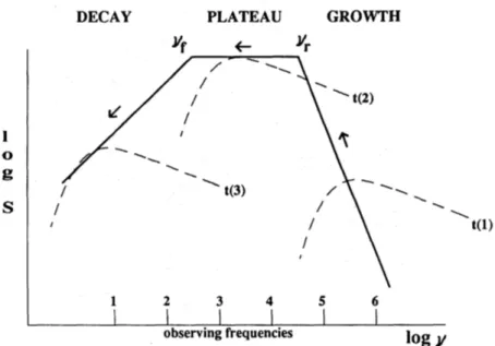
Up to now we have seen the various types of AGN observed and the various processes that produce the observed spectra in a specific time. Variability though have been ob- served from the early observations of AGNs with observed time scales of months, years or even minutes are frequently observed. The rapid blazar variability, probes spatial scales inaccessible even to interferometric imaging and has been explained in terms of e.g. rel- ativistic shock-in-jet models (e.gMarscher and Gear 1985;Valtaoja et al. 1992a,b;Stevens et al. 1994;T ¨urler 2011) or colliding relativistic plasma shells (e.g.Spada et al. 2001;Guetta et al. 2004). Quasi–periodicities seen in the long term variability curves on time scales of months to years, may indicate systematic changes in the beam orientation (Camenzind and Krockenberger 1992), possibly related to binary black hole systems, MHD instabili- ties in the accretion disks and/or helical/precessing jets (e.g.Begelman et al. 1980;Villata and Raiteri 1999;Chen et al. 2013). Bellow a short description of the shock in jet model is presented.
1.5.1 Shock–in–Jet model
The classical shock in a jet model of Marscher and Gear(1985);Valtaoja et al.(1992a,b);
Stevens et al.(1994);T ¨urler (2011) assumes a shock wave propagating through a conical
1.5 Variability of Blazars 11 jet accelerating relativistic particles at the shock front (Fig.1.7), while travelling behind the shock front these particles loose energy due to different mechanisms i.e. Compton synchrotron and adiabatic losses. The three distinct evolutionary stages can be described as follows:
Figure 1.7:Representation of a the shock in jet model. (image from:T ¨urler(2011))
the growth stage: The first is called the Compton stage due the dominant energy losses by Compton scattering. It is characterised by the increase of the observed turnover flux density and the decrease of the turnover frequency. This stage can be described by the following relations :
Sm νm11 α 2α 1 (1.8a)
νm R α 1 4 (1.8b)
where:
Sm : is the flux density at the turnover frequency νm : is the self absorbed turnover frequency α : is the spectral index
R : is the distance from the vertex of the cone
the plateau stage: The second is called the synchrotron stage were energy losses are dom- inated by synchrotron losses of the electrons. It is characterized by and almost constant value of the turnover flux density and the decay of the turnover frequency. The behaviour of the turnover flux density and frequency can then be described by :
Sm νm2s 5 2 3α 4s 2 3αs 1 (1.8c)
νm R 4s 2 3αs 1 3s 5 (1.8d)
where s is the slope of the spectral energy distribution.
the decay stage: The third and last is called the adiabatic stage and refers to energy losses due to adiabatic expansion. It is characterized by the decrease of both the turnover fre- quency and flux. In that case the above relations become :
Figure 1.8:Prototype behaviour according to the generalized shock–in jet model ofValtaoja et al.
(1992b)
Sm νm10s 1 7s 8 (1.8e)
νm R 7s 8 3s 4 (1.8f)
These three stages are demonstrated in Fig.1.8, tracing the self-absorbed turnover fre- quency of the shock spectrum as it evolves in the frequency-flux space. The standard Marscher and Gear(1985) model assumes a constant Doppler factor whereas the latter can strongly influence the slopes of the different evolution stages in the Smax–νmaxplane. This model is the basis that the generalized shock in jet model ofValtaoja et al.(1992b) is based upon.
1.5.2 Geometrical models
Apart from shock in jet model described above also geometrical effects can modulate the observed emission and can introduce variations in flux density on different long term time scales. One possible explanation is the emission regions moving alongside bend radio structures. Such bend jets are frequently found (e.gAgudo et al. 2012;Lobanov and Zen- sus 2001;Ly et al. 2007;Piner et al. 2009;Camenzind and Krockenberger 1992). Several the- oretical models exist i.e. oscillating bent jets, helical modes in hydrodynamic jets (Hardee
1.6 F-GAMMA Program description 13
1987) or in magnetized jets (Konigl and Choudhuri 1985). The basic idea is that when- ever an emission feature moves along alongside the helical or bend structures differential Doppler boosting occurs producing the observed variability.
1.6 F-GAMMA Program description
F-GAMMA stands for Fermi Gamma-ray Space TelescopeAGN Multi-frequency Moni- toringAlliance and comprises the coordinated efforts of a broad consortium of scientific groups and observatories with the aim to collect (quasi-) simultaneous and high–precision broadband monitoring data (total intensity and polarization) for a large number ofγ–ray sources in the ’‘low-energy” synchrotron part of blazar SEDs. Monthly monitoring obser- vations are performed for about 60 sources at frequencies between 2.6 and 345 GHz with the Effelsberg 100–m (EB), Pico Veleta 30–m (PV) and APEX 12–m telescopes including polarization at several bands.
Scientific motivation and goals of the program
Figure 1.9:The F-GAMMA program logo.
As already mentioned Blazars (FSRQs and BL Lacs) as AGN sub–class exhibit extreme phenomenological characteristics such as rapid broadband flux density and polariza- tion variability, high degree of polarization and a broadband, double–humped spectral energy distribution (SED) (e.g.Urry 1999).
The recent discovery of blazars as a group of bright and highly variable high energy γ–ray sources (Hartman et al. 1992) ex-
panded our knowledge but many questions remain unanswered. Is the jet composition leptonic or hadronic and which are the emission processes? What is the origin of their often violent broadband variability? Where in the jet are the high energyγ–ray photons produced? Is the production region located at the jet–foot point close to the SMBH or at several parsecs downstream?
The launch of theFermi Gamma-ray Space Telescope ((Fermi–GSTMichelson 2008) in June 2008, along with the Large Area Telescope detector (LAT,Atwood et al. 2009) on board Fermi and its dramatically improved capabilities compared to its predecessor EGRET, is providing spectacularγ–ray light curves and spectra resolved at a variety of time scales for a large number of AGN during the first years of operation (Abdo et al. 2009a,2010b;
Ackermann et al. 2011).
The new era in AGN astrophysics introduced by Fermi-GST will help answer still open questions, in particular the production and location of the γ–ray emission as well as the origin of the rapid (time scales of days to months/years) variability of the syn- chrotron and IC branch. The observed rapid blazar variability as already mentioned is
attributed to either intrinsic variability or geometrical models. Variability studies give important clues about the size, structure, physics and dynamics of the emitting region making AGN/blazar monitoring programs of uttermost importance in providing the nec- essary constraints for understanding the origin of energy production.
Detailed long term monitoring data sets of large source samples are rare at cm and short–mm bands. In this framework, and in order to fully explore the opportunities opened up byFermi–LAT, the F-GAMMA monitoring program (Fuhrmann et al. 2007;Angelakis et al. 2010b;Fuhrmann et al. 2014;Angelakis et al. 2015) was initiated in 2007, monitoring the variability and spectral evolution of 60Fermibright sources at frequencies between 2.6 and 345 GHz. It is the first AGN radio monitoring program that covers such a large frequency range in a highly homogeneous and coordinated manner.
Participating facilities and groups
The core facilities of the F-GAMMA program are the EB and the PV telescopes. A full and detailed description of the observations performed in these two telescopes is given in Sect.2, Sect.3.1.1and Sect.3.3.1.
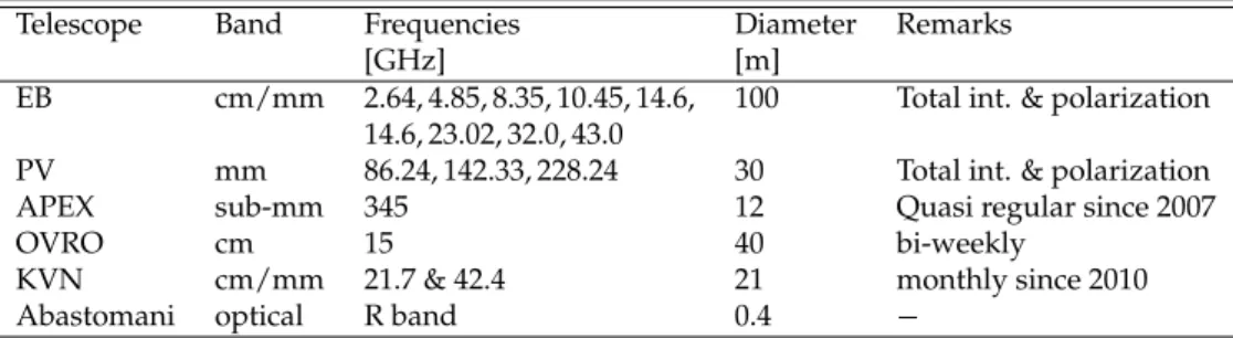
The F-GAMMA program is closely collaborating with a large number of other obser- vatories, programs and teams in the AGN community. A summary of all the participating facilities is shown at Table1.2. More specifically :
• the APEX 12-m telescope
Since 2008, the bolometer array LABOCA (Siringo et al. 2008) of the APEX 12-m telescope to obtain complementary observations at a frequency of 345 GHz. Quasi- regular flux density measurements are performed during several dedicated APEX LABOCA time-blocks per year. These, however, are not coordinated with the EB and PV measurements and instead depend on the scheduling of the regular LABOCA sessions. At APEX, a sub-sample of 25γ-ray blazars of the F-GAMMA sample are observed together with a sample of 14 southern hemisphereγ-ray AGN. Details in- cluding the first five years of data will be presented in Fuhrmann et al. (in prep). (see alsoLarsson et al. 2012).
• the Caltech/OVRO 40-m monitoring program
In 2007 a program complementary to F-GAMMA was commenced at the OVRO 40-m telescope. It is monitoring a statistically complete sample of about 1200 blazars. This sample also includes all the sources that are monitored by the F-GAMMA program.
The observations are performed at least twice a week making it a perfect companion to the monthly observations of the F-GAMMA program. For more details see also Richards et al.(2011)
• Abastomani Observatory optical monitoring program
Abastomani Observatory observes a large sample of AGN since 1997 at the optical R band using the 70-cm and 125-cm telescopes (Kurtanidze et al. 2009). There is a large
1.7 Scope of current thesis 15
overlap in monitored sources with the F-GAMMA sources.
• Korea Astronomy and Space Science Institute: monitoring program with the KVN
An F-GAMMA collaboration has been established with the Korean VLBI Network (KVN) team using the KVN antennas for single-dish monitoring ofγ-ray loud blazars at 22 and 42 GHz in total intensity and polarisation. The program started in 2010 and is performed monthly including most of the F-GAMMA sources.
Table 1.2:List of participating telescopes and projects in the F-GAMMA program.
Telescope Band Frequencies Diameter Remarks
[GHz] [m]
EB cm/mm 2.64, 4.85, 8.35, 10.45, 14.6, 100 Total int. & polarization 14.6, 23.02, 32.0, 43.0
PV mm 86.24, 142.33, 228.24 30 Total int. & polarization
APEX sub-mm 345 12 Quasi regular since 2007
OVRO cm 15 40 bi-weekly
KVN cm/mm 21.7 & 42.4 21 monthly since 2010
Abastomani optical R band 0.4
1.7 Scope of current thesis
The lack of continuous observations at a wide range of spectral bands and the lack of suf- ficiently dense sampled and long–term monitoring data prevented the detailed study of the broadband jet emission in the past. The analysis performed for the thesis in hand is ac- complished within the framework of the F-GAMMA program, analysing the variability of light curves and quasi-simultaneous spectra of the first five years of F-GAMMA observa- tions, allowing a detailed study of the broadband emission characteristics and variability scenarios.
While cm variability is believed to originate mainly at the outer parsec scales of jets, at higher frequencies the lower source intrinsic opacity allows a deeper and less obscured look into the central engine. Consequently, the variability in the mm bands probes the pro- cesses in the ultimate vicinity of the core and allows a far more direct study of the physics of the central engine than possible at cm bands. In the current thesis cm and short–mm variability is studied as a whole allowing for the first time to study the evolutionary paths of flares from frequencies as high as 142 GHz down to 2.6 GHz for such a large number of sources. Variability characteristics (amplitudes and time scales) and spectral characteris- tics (spectral indices, Smax–νmaxflare peak analysis ) are presented along with estimations of brightness temperatures and Doppler factors. The thesis is organized as follows:
Chapter 2 provides general information of the source sample characteristics and the dataset that is used for the analysis. The observing methods utilized for observations performed at EB and PV , as well as a cross calibration study of the two aforementioned telescopes. Finally information the observing logistics is provided.
Chapter3presents the data reduction methods and post measurement corrections ap- plied to the data acquired with EB and PV alongside with a detailed error budget analysis and a detailed study of the PV telescope system.
Chapter4describes the analysis tools and methods that are applied to the light curves and broadband spectra to obtain information such as: variability characteristics, flare am- plitudes, flare time scales, spectral indices and spectral peak estimations.
Chapter5 presents the results in the time domain of the analysis performed upon the five year of EB and PV combined light curves. The significance of variability through a χ2 test is estimated as well as the flare amplitudes using a new analysis method for the estimation of the intrinsic variability of the light curves along with a new proposed k–index to quantify the variability across frequency. Finally flare time scales, brightness temperatures and Doppler factors are reported.
Chapter6presents the corresponding analysis in the spectral domain, including results for spectral indices and an Smax–νmaxanalysis.
FinallyChapter7provides the overall discussion and summary of the obtained results and the contribution of the thesis at hand. Finally a short description of future studies that can be based on the results obtained here is provided.
2
Observations
2.1 The Source sample
Since January 2007 the F-GAMMA program has been monitoring about 60 sources on a monthly basis, consisting of the most prominent, famous, frequently active, and usually strong blazars. In June 2009 a revision of the sample took place making the total number of sources that were ever observed within the program 90. The source sample that is used for the analysis presented here consists of the 59 sources of the revised F-GAMMA sample. The selection criteria of the original and the revised samples can be summarized as follows:
The original F-GAMMA sample: The F-GAMMA source sample observed between January 2007 and June 2009 consisted of 69 sources with a declination limit ofδ 30 . A large fraction of these sources were selected on the basis of their previousγ–ray detec- tion with the EGRET detector on board the Compton Gamma Ray Observatory (CGRO) and their presence in the “high priority” AGN/blazar list announced by theFermi-LAT AGN group (Fuhrmann et al. 2007). Furthermore, the source selection was done so that a maximum overlap with existing cm and mm VLBI and other programs of similar kind is achieved. Of the 61 original sources monitored at PV , 35 sources were also part of the more general monitoring conducted by IRAM.
The revised F-GAMMA sample: After the launch and the first year ofFermi-GST oper- ations a revision of the original sample was performed in June 2009 to exclusively include Fermi-GST detected sources. Specifically, 38 sources of the revised sample have already been in the original sample, while 31 have been replaced by newFermiγ-ray sources. 34 sources are part of the more general monitoring conducted by IRAM. Furthermore, some of the new sources have data prior to June 2009, thanks to the IRAM program. The original
and revised samples are presented in TablesA.1andA.2along with some basic informa- tion.
It must be noted that the described F-GAMMA samples are not constructed accord- ing to strict selection criteria and are thus statistically incomplete. Generalizations of any findings must be made with caution. To address the incompleteness of the source sam- ple and to enable statistically robust population studies of the variability properties of blazars, a statistically complete parent sample is needed. For this purpose sources located atδ 20 where selected from CGRaBS (Healey et al. 2008) and are observed about twice each week at 15 GHz within the OVRO 40 m monitoring program (Richards et al. 2009).
2.1.1 Redshift distribution of F-GAMMA Blazars
For several studies that follow (Chapters6and5) the knowledge of redshift (z) for mon- itored sources is important. The distribution of z for the revised sample for the FSRQs and BL Lacs is presented in Fig.2.1. It is clear that FSRQs are systematically farther away compared to BL Lacs as expected. The mean value of z for all the sources in the sample is 0.77 with a median of 0.66 , while FSRQs exhibit a mean value of 1.18 and median of 1.14 and BL Lacs a mean value of 0.29 and median of 0.19.
0 0.3 0.6 0.9 1.2 1.5 1.8 2.1 2.4 2.7 3 3.3 3.6 3.9 Redshift
0 2 4 6 8 10 12 14 16 18 20 22 24 26 28
Number of sources
All sources FSRQs BLLacs Other
Figure 2.1:Redshift distribution of F-GAMMA blazars. All sources in Grey, BL Lacs in Red, FSRQs in Black and other types in Green.
For any physical quantities that are estimated from the analysis done for the current thesis (e.g brightness temperatures, Doppler factors, k-index), the redshift distribution is taken into account.
2.1.2 The Dataset
The dataset used for the following analysis covers the period from January 2007 to January 2012 i.e. the first five years of F-GAMMA observations. All sources in the revised sample