Structure of Hot Molecular Cores

(1)

Structure of Hot Molecular Cores

I n a u g u r a l - D i s s e r t a t i o n

zur

Erlangung des Doktorgrades

der Mathematisch-Naturwissenschaftlichen Fakult¨at

der Universit¨at zu K¨oln

vorgelegt von

Rainer Rolffs

aus Bonn

(2)

(Gutachter)

Prof. Dr. Karl Menten

Tag der m¨undlichen Pr¨ufung: 22. 6. 2011

(3)

Zusammenfassung

Massereiche Sterne entstehen tief im Inneren von dichtem molekularem Gas, welches sie aufgrund ihres hohen Energieausstoßes aufheizen und ionisieren. Während einer frühen Phase ist die Ionisation auf kleine Bereiche beschränkt und die stellare Strahlung wird von Staub absorbiert. Die hohen Temperaturen führen zum Verdampfen der Eismäntel der Staubkörner, und viele hoch angeregte und komplexe Moleküle können in diesen heißen molekularen Kernen beobachtet werden. In späteren Stadien wird die ganze Molekülwolke ionisiert und auseinanderge- rissen, und ein Sternhaufen wird sichtbar.

Diese Doktorarbeit hat zum Ziel, die Verteilung von Dichte, Temperatur, molekularer Häufigkeit und Ge- schwindigkeitsfeld in heißen molekularen Kernen näher zu bestimmen. Diese Schlüsselinformationen für die Entstehung massereicher Sterne und für die Astrochemie werden durch aufwendige Strahlungstransport-Modellie- rung sowohl von Einzelteleskop- als auch von Interferometer-Beobachtungen gewonnen.

Zwölf Quellen wurden mit dem APEX-Teleskop in Submillimeter-Linien der Moleküle HCN, HCO⁺und CO beobachtet, wobei ein weiter Bereich von Anregungen und optischen Tiefen abgedeckt wurde. Dies wurde mitt dem Herschel-Teleskops ergänzt, welches HCN-Linien in SgrB2-M bis zu hohen (THz-) Frequenzen und Anregun- gen beobachtete. Die Linienformen und -intensitäten wurden mit dem sphärischen Strahlungstransportprogramm RATRAN unter den Annahmen einer radialen Potenzgesetz-Verteilung der Dichte und eines zentralen Heizens modelliert.

Vibrationsangeregtes HCN und ionisiertes Gas wurden mit dem VLA-Radiointerferometer bei einer hohen Auflösung von 0.1^′′ (1000 AU) in G10.47+0.03, SgrB2-M und -N kartiert. Das SMA-Interferometer wurde eingesetzt, um Hunderte von Moleküllinien und Staubemission in G10.47+0.03 zu beobachten, wobei eine Fre- quenz von 690 GHz und eine Auflösung von 0.3^′′erreicht wurden. Die Daten wurden mit dem dreidimensionalen Strahlungstransportprogramm RADMC-3D modelliert, welches die Staubtemperatur aus dem stellaren Aufheizen berechnet.

Modellieren mit einer Potenzgesetz-Dichtestruktur reproduziert die meisten Einzelteleskop-Linien, aber die hochaufgelösten Daten zeigen eine zentrale Abflachung und eine schnelle radiale Abnahme der Dichte und ähneln einem Plummer-Profil. Das Modellieren der Linienformen deutet auf kleinskalige Dichteschwankungen hin. In- ternes Heizen durch massereiche Sterne ist konsistent mit den Daten und macht sich durch vibrationsangeregtes HCN um kleine Regionen von ionisiertem Gas bemerkbar. Strahlungsdiffusion aufgrund der hohen Säulendichten führt zu Hunderten von Sonnenmassen an heißem (>300 K) Gas. Die HCN-Häufigkeit nimmt mit der Temperatur zu und erreicht in heißem Gas hohe Werte der Größenordnung 10⁻⁵ relativ zu H2. Großskaliger Einfall macht sich durch asymmetrische Linienformen bemerkbar und ist langsamer als der freie Fall, während zur selben Zeit zentrale Expansionsbewegungen durch blauverschobene Absorption und eine sich mit höherer Anregung ändernde Asymmetrie nachgewiesen sind.

Ich stelle fest, dass heiße molekulare Kerne bei anhaltendem Gravitationseinfall durch die beginnende Rück- kopplung massereicher Sterne auf das Gas gekennzeichnet sind. Der erhöhte thermische, turbulente, windgetriebene und Strahlungsdruck im zentralen Bereich führt zu Expansionsbewegungen und zu einem zentralen Abflachen der Dichte. Hohe Temperaturen werden mittels Diffusion der Strahlung durch Staub erreicht.

5

(8)

(9)

Abstract

High-mass stars form deeply embedded in dense molecular gas, which they heat up and ionize due to their high energy output. During an early phase, the ionization is confined to small regions, and the stellar radiation is absorbed by dust. The high temperatures lead to the evaporation of ice mantles around dust grains, and many highly excited and complex molecules can be observed in these Hot Molecular Cores. At later stages, the whole molecular cloud is ionized and disrupted, and a star cluster becomes visible.

This PhD thesis aims at constraining the distribution of density, temperature, molecular abundances, and velocity field in Hot Molecular Cores. This key information for high-mass star formation and for astrochemistry is obtained by sophisticated radiative transfer modeling of both single-dish and interferometric observations.

With the APEX telescope, 12 sources were observed in submillimeter lines of the HCN, HCO⁺, and CO molecules, covering a wide range of excitations and optical depths. This was extended with the Herschel space telescope, which observed HCN lines in SgrB2-M up to high (THz) frequencies and excitations. The line shapes and intensities were modeled with the spherical radiative transfer code RATRAN, assuming a radial power-law density distribution and central heating.

With the VLA radio interferometer, vibrationally excited HCN and ionized gas was mapped at a high resolution of 0.1^′′(1000 AU) in G10.47+0.03, SgrB2-M and -N. The SMA interferometer was used to observe hundreds of molecular lines and dust emission in G10.47+0.03, reaching a frequency of 690 GHz and a best resolution of 0.3^′′. The data were modeled with the three-dimensional radiative transfer code RADMC-3D, which computes the dust temperature from stellar heating.

Modeling using a power-law density structure reproduces most single-dish lines, but the high-resolution data show a central flattening and a rapid radial decrease of the density, resembling a Plummer profile. Modeling of the line shapes indicates small-scale clumpiness. Internal heating by high-mass stars is consistent with the data and traced by vibrationally excited HCN around small regions of ionized gas. Diffusion of radiation due to the high column densities lead to hundreds of solar masses of hot (>300 K) gas. The HCN abundance increases with temperature, reaching high values on the order of 10⁻⁵relative to H₂in the hot gas. Large-scale infall is traced by asymmetric line shapes and is slower than free-fall, while at the same time central expansion motions are detected by blue-shifted absorption and a change of the asymmetry with higher excitation.

I conclude that Hot Molecular Cores are characterized by the beginning feedback from high-mass stars, while gravitational infall is ongoing. The increased thermal, radiative, turbulent, and wind-driven pressure in the central region leads to expansion motions and to a central flattening of the density. High temperatures are reached through diffusion of radiation by dust.

7

(10)

(11)

Chapter 1

Introduction

This PhD thesis was conducted at the Max-Planck-Institut f¨ur Radioastronomie in Bonn and the I. Physikalisches Institut at the University of Cologne. I worked on it from March 2008 to April 2011. The thesis advisor was Peter Schilke.

This introductory chapter gives background information and highlights the scientific context of the thesis, which is high-mass star formation. Starting from the conditions for star formation (Sect. 1.1), the peculiarities of the formation of high-mass stars are described in Sect. 1.2. Section 1.3 gives details about Hot Molecular Cores, an evolutionary stage of high-mass star formation prominent for molecular line emission. Problems in observations, analysis, and theory are discussed in Sect. 1.4. Finally, the aims of this thesis are defined in Sect. 1.5.

The next chapter (Chapter 2) describes the tools used in this work. As the measurement of electromagnetic radiation plays a key role for the whole science of astronomy, the first part (Sects. 2.1 to 2.4) is about radiative transfer, with an emphasis on molecular lines. Section 2.5 describes the observational techniques to measure radio and submillimeter wavelengths (single-dish and interferometry), and Sect. 2.6 introduces the modeling tools that are used to analyze the observational data. They basically simulate the radiative transfer and the observations of a model, to be compared to the real data.

Chapters 3 to 6 form the main part of the thesis. They rely on observations made with the APEX 12-m telescope (Chapter 3), the Herschel Space Observatory (Chapter 4), the VLA radio interferometer (Chapter 5), and the SMA submillimeter interferometer (Chapter 6). I present and discuss the observational data and the analysis with radiative transfer modeling in these chapters. They are based on papers that I have written. The papers of Chapters 3, 4, and 5 are refereed and published in the journal Astronomy&Astrophysics (Rolffs et al. 2011b, 2010, 2011a), the paper of Chapter 6 (Rolffs et al. 2011c) is submitted to the same journal. To Chapter 7 I contributed only the modeling part (Sect. 7.5), but reproduce the whole letter submitted to A&A (Qin et al. 2011) in order to embed Sect. 7.5 in its context.

In Chapter 8, I discuss the results from all observations and modeling, focusing on heating (Sect. 8.1), the density distribution (Sect. 8.2), the velocity field (Sect. 8.3), and the implications for astrochemistry (Sect. 8.4) and high-mass star formation (Sect. 8.5). Finally, I draw conclusions in Chapter 9 and give a short outlook in Chapter 10.

1.1 Pressure in the Interstellar Medium

The Interstellar Medium (ISM) is kept in the plane of the Galaxy by the gravitational potential of the stars. In addition, the dense (molecular) clouds are held together by self-gravity. Turbulence plays an important role on all scales, rendering the ISM highly dynamic (e.g. Ballesteros-Paredes et al. 1999; Mac Low & Klessen 2004). This is in contrast to the old picture of pressure equilibrium (Spitzer 1978), which is characterized by stable phases.

1.1.1 Heating and Cooling

The temperature of the ISM depends on (past and present) heating and the efficiency of cooling. Heating is basically the conversion of other forms of energy into thermal energy, which is genererally backed by the tendency to increase the entropy. Cooling is the conversion of thermal energy into photons, which are dispersed in space. It depends on the temperature, while heating is independent of it.

Above 10⁶ K, the gas cools slowly by free-free radiation. At lower temperatures, internal levels of the gas particles have to be excited by collisions to decay radiatively, which depends on the availability of levels that can be excited. Above 10⁴K, electronic levels of atoms and ions are easily excited, and cooling is very efficient, but

9

(12)

lower temperatures are not sufficient to excite these levels. Excitation of fine-structure lines, such as the C⁺line at 158µm, can cool down to about 100 K.

The formation of molecules starts the next step of cooling by providing further efficient mechanisms. As molecules have many low-lying rotational (and vibrational) levels, the gas can cool e.g. by rotational transitions of CO and H2O. In addition, dust (about 1% of the mass) cools by continuum radiation, and influences the gas temperature through collisions with the molecules, especially at high density.

Main heating sources of the ISM are stellar radiation and supernovae. The first provides an approximately constant heating through absorption of the local interstellar radiation field. The latter is a rare explosive event, inducing not only radiation energy, but especially kinetic energy. Shocks and the decay of turbulence subsequently heat up the gas. In dense molecular clouds, which are shielded from the interstellar star light, absorption of the cooling radiation itself, the conversion of gravitational energy, and cosmic rays provide additional heating, maintaining a minimum temperature of about 10 K, typical before the onset of star formation.

Considering the efficiency of cooling and heating by stellar radiation, three phases can be distinguished in a simplified picture of the ISM (McKee & Ostriker 1977) - a hot ionized phase of 10⁶K produced by supernovae, a warm phase of 10⁴K (which can have different degrees of ionization), and a cold neutral phase of about 100 K. The thermal pressure, which is the product of particle density and temperature, would be nT ≈3000 cm⁻³K outside of molecular clouds (where gravity is crucial), leading e.g. to a few dozen atoms per cm³for the cold phase. The volume of the Milky Way is thought to be about equally distributed between the hot and the warm phase, the gas mass (∼10¹⁰M_⊙¹) between the warm and the cold phase.∼10% of the gas mass is molecular.

The modern picture emphasizes much more the turbulent and dynamic nature of the ISM, which is out of equilibrium. The lifecycle of interstellar matter involves gradual cooling and contracting until star formation sets in, and subsequent heating and disruption of the remaining gas. Through star formation, the ISM loses mass, which could be partly replenished from the intergalactic medium.

1.1.2 Collapse

Pressure gradients drive the acceleration of matter. Different types of pressure can be distinguished, e.g. thermal, gravitational, turbulent, rotational, or magnetic pressure. Gravity is the driving force for collapse, while most pressure types provide support against collapse. Turbulence provides support on global scales, but can promote local collapse at the same time (Klessen et al. 2004).

At high densities, self-gravity becomes important, exerting a contraction force. Thermal and turbulent pressure represent microscopic and macroscopic motions of the particles, respectively. In addition, magnetic pressure tends to stabilize a cloud against collapse, since charged particles are coupled to the magnetic field, which resists compression. Neutral and charged particles can slowly decouple by ambipolar diffusion.

For collapse to occur, gravity has to ultimately win over all other forces. A simple approximation to estimate the critical mass, at which the cloud is stable, is to evaluate the energy balance in virial equilibrium

2T +2U+M+W=0 (1.1)

For a cloud of mass M and radius R, the internal energy (kinetic energy of macroscopic motion) isT ∝ Mv² with v the typical velocity, the thermal energy isU ∝MT , the magnetic energy isM ∝B²R³with the field strength B, and the gravitational (or potential) energy isW ∝ −^MR². For collapse, the gravitational energy must be larger than the rest. However, this is very simplified and ignores surface terms, also it is not always clear if the condition of equilibrium is fulfilled (Ballesteros-Paredes 2006).

A simple case is to consider only gravitational and thermal energy: Then U ∝ W, or T ∝ ^MR, therefore M ∝ρR³∝ρ^M_T₃³. Division by M and multiplication by ^T_ρ³ leads to the Jeans mass M_J ∝ q

T³

ρ. For a temperature of 10 K and a density of 10⁴H2 molecules per cm³, it is about 1 M_⊙, while for diffuse neutral gas it can be some 10⁴M_⊙.

In the complete absence of supporting forces, a cloud would collapse over the free-fall time t_ff. The core radius R is roughly the acceleration times the square of this time, R ≈ ^GM_R2t²_ff, so t_ff ≈ (Gρ)⁻¹². For a neutral cloud, the free-fall time is around 10⁷years, for a dense core only some 10⁴years.

With increasing density, self-gravity becomes stronger. Smaller masses can collapse and the timescales are shorter. Collapse thus proceeds first in the dense, inner regions, with outer regions following (inside-out collapse, Shu 1977). This might be different if the cloud is initially homogeneous, in which case the collapse propagates inward (Larson-Penston collapse, Larson 1969a; Penston 1969). A comparison between these solutions can be found in Zhou (1992).

1Astronomical constants in this thesis are solar mass M_⊙=1.98892×10³⁰kg, solar luminosity L_⊙=3.839×10²⁶W, the Astronomical Unit AU=1.49598×10¹¹m, and the parsec pc=3.08568025×10¹⁶m. Physical constants are Planck’s constant h=6.626×10⁻³⁴Js, the speed of light c=2.99792458×10⁸m/s, Boltzmann’s constant k=1.38×10⁻²³J/K, and the gravitational constant G=6.6739×10⁻¹¹m³/kg/s².

(13)

1.2. HIGH-MASS STAR FORMATION 11 The supporting force is here represented by thermal pressure. However, in molecular clouds turbulence and magnetic fields dominate, increasing the stable mass. The far greater contribution of turbulence than of thermal pressure can be seen in the line widths, which are much larger than the thermal line width. The line width to the power of three is contained in the Jeans mass.

Nevertheless, since higher densities increase the self-gravity, the stable mass decreases and consecutively lower masses can contract. This is triggered by turbulent contractions. This gravoturbulent fragmentation leads to strong density fluctuations (cores inside clumps) in Giant Molecular Clouds, which typically measure 50 pc and have masses of 10⁵M_⊙. Molecular clouds are probably in a non-equilibrium state of overall gravitational collapse with many local centers of collapse (Ballesteros-Paredes et al. 2011).

Collapse first proceeds in an isothermal way, as the energy released by contraction, converted to thermal energy, can be radiated away easily. This is essential for the fragmentation. However, as the density increases, it becomes harder to get rid of the additional thermal energy, because cooling lines become optically thick, leading to trapping of line photons, and later also the dust emission is increasingly absorbed. The dust optical depth becomes even larger with higher temperature, as the emitted radiation is shifted to shorter (infrared) wavelengths.

When the isothermal approximation breaks down due to the large dust optical depth, the collapsing core can cool only at its surface, where accretion is ongoing, and the temperature rises. A first hydrostatic core develops, where thermal pressure balances gravity (Masunaga et al. 1998). This is the seed of a star.

1.1.3 Expansion

As soon as stars have formed, they provide additional pressure to the ISM. They convert gravitational and nuclear binding energy into radiation, produce winds and, during the accretion, bipolar outflows.

These feedback mechanisms strongly enhance the turbulence and also the thermal pressure by heating the gas.

Especially the high-mass stars also provide radiation pressure and ionize the surrounding gas by their strong UV radiation. The ionized gas has high pressure due to its temperature of 10⁴K. The combined pressure from the fast stellar winds that high-mass stars drive, their radiation pressure, and the thermal pressure of the ionized gas finally removes the gas from a newly formed star cluster. Having lost a substantial part of their mass, the less massive clusters disssolve.

The feedback on the star formation process itself is mostly negative, since the additional pressure works against gravity. However, it can also be positive and trigger star formation elsewhere by compressing the gas locally (Deharveng & Zavagno 2008; Zavagno et al. 2007, 2010).

At later stages of stellar evolution, massive winds can lead to an expansion of stellar envelopes, and high-mass stars explode after a few million years as supernovae, sweeping up and heating the ISM on large scales. These processes enrich the ISM with metals and close the cycle of interstellar matter.

1.2 High-Mass Star Formation

A detailed overview of star formation, including also the topic of the last section (Sect. 1.1), can be found in the book by Stahler & Palla (2005). A review on high-mass star formation is Zinnecker & Yorke (2007).

1.2.1 Impact

The formation of high-mass stars, through its feedback on the ISM, regulates the star formation process. Together with the high energy output, it thus shapes and dominates the evolution and appearance of galaxies. This is particularly true for starburst galaxies and earlier cosmic epochs, which were characterized by high star formation rates triggered by galaxy mergers. The first stars in the universe must have had very high masses, as the gas temperatures were high due to the lack of cooling mechanisms. Mainly through the production and disposal of heavy elements, high-mass stars provide the conditions for the formation of dust, planets, and life.

High-mass stars have large enough masses that they collapse to a neutron star or a black hole when the raw material of nuclear fusion is exhausted and its support against gravity vanishes. The released potential energy causes a supernova explosion, outshining the whole galaxy and creating giant bubbles in the ISM. This criterion means that they have masses above∼8 M_⊙. According to the stellar initial mass function (IMF, Kroupa 2002), only 0.4% of newly formed stars have high enough masses. However, as the luminosity on the Main Sequence (MS, which relates the luminosity to the surface temperature of hydrogen-burning stars) is proportional to the mass to the power of about 3.5, they dominate the luminosity, but use up the hydrogen fuel very quickly (lifetime on the MS proportional to M/L, about 10¹⁰ years for the Sun). So high-mass stars are short-lived, and most of their material is recycled to the ISM. In contrast, the matter is essentially locked in the 94% of newly formed stars that have masses lower than 1 M_⊙.

(14)

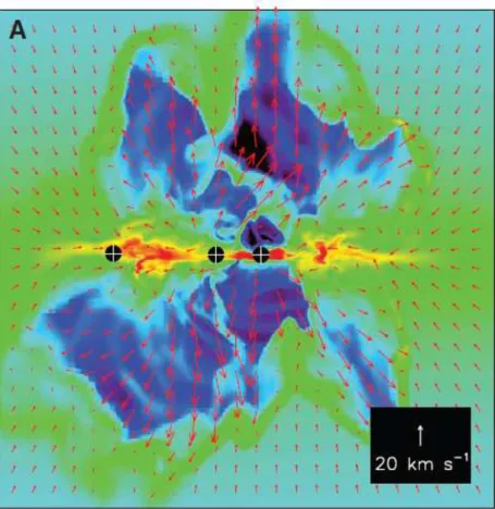
Figure 1.1: High-mass stars forming via disk accretion (simulation by Krumholz et al. 2009). The color scale represents logarithmic density, the arrows denote the gas velocity.

Already before the supernova explosions, high-mass stars have a far greater impact on their natal molecular cloud than the low-mass stars. They have high luminosities and hot surface temperatures, therefore an ionizing radiation field, producing Hiiregions and photon dominated regions (PDR), where the molecules are dissociated.

With their fast winds, they drive out the cluster gas.

1.2.2 Accretion

A fundamental difference between low-mass and high-mass star formation is that for low-mass stars hydrogen burning starts only after accretion and contraction have finished, while for high-mass stars it starts while still growing in mass. The virial equilbrium (Equation 1.1), which applies to a hydrostatic core, relates gravitational and thermal energy; hence contraction and higher mass mean higher temperatures, which eventually ignite hydrogen.

For high-mass star formation, the Kelvin-Helmholtz time scale R/R˙ = ^GM_RL², over which the luminosity could be maintained by contraction, is less than the collapse time scale M/M. The accretion rate ˙˙ M (infalling mass per time) produces a luminosity of ^GM_R M. It depends on stellar mass and environment, and a high-mass star reaches values˙ over 10⁻³M_⊙yr⁻¹(Beuther et al. 2002; Keto & Wood 2006).

The extreme luminosities of high-mass stars lead to high radiation pressure, which reverses any spherical accretion flow. Therefore, they can only form by an inhomogeneous non-spherical infall or by disk accretion.

This way, the accreting material is shielded from the radiation, which can escape through expanding low-density bubbles (e.g. Fig. 1.1, Krumholz & Matzner 2009).

Disk accretion is accompanied by bipolar outflows. In low-mass star formation, magneto-centrifugal outflows, powered by the accretion, are a common phenomenon. High-mass stars produce strong radiation-driven winds, which can entrail molecular gas in an outflow.

Outflows from young high-mass stars are much more massive (Beuther et al. 2002) and probably less collimated (Shepherd 2005) than from low-mass stars. Direct detection of disks is more difficult. Large massive but instable rotating structures, so-called toroids, have been observed (Beltr´an et al. 2005; Cesaroni et al. 2007).

The ionization is first quenched by accretion, i.e. the accretion rate is larger than the ionization rate and so no Hiiregion can be observed (Walmsley 1995). Accretion, with its large infalling momentum, can well proceed into Hiiregions as an ionized accretion flow (Keto 2003). Finally, the accretion disk is probably photoevaporated,

(15)

1.3. HOT MOLECULAR CORES 13 which puts an end to accretion (Hollenbach et al. 1994), and the Hiiregion undergoes the classical pressure-driven expansion (Spitzer 1978).

That accretion must occur through a disk is also set by the conservation of angular momentum. Forming stars have to get rid of angular momentum, which would prevent contraction otherwise. Therefore, matter has to flow in while angular momentum is transported outwards by friction in the disk or by outflows. Also the formation of binary or multiple stellar systems and of planets serve this purpose.

In addition to angular momentum, other factors limit and regulate star formation, whose relative importance is not clear though. Important contributions come from turbulence (Mac Low & Klessen 2004), likely replenished by outflows (Li & Nakamura 2006; Wang et al. 2010), and from magnetic fields (e.g. Hennebelle & Fromang 2008;

Peters et al. 2011). Also thermal pressure from heating, winds, and radiation pressure play a role.

While it has become clear that high-mass stars can form by accretion, although with substantial differences to low-mass stars, it is currently under debate how high-mass stars grow by accretion, with two rivaling theories.

Monolithic collapse of turbulent-supported cores (McKee & Tan 2003) assumes that a high-mass star has its own well-defined mass reservoir and accretion disk. In contrast, competitve accretion in a cluster environment (Bonnell et al. 2001, 2004) focuses on the global mass reservoir, accreted by the combined gravitational potential of the stars, which compete for this accretion flow by their location and their mass.

There is observational support for both scenarios, e.g. the outflows and the core mass function for monolithic collapse and the large-scale infall and the clustering of high-mass stars for competitive accretion. The truth lies probably in between, with aspects of both theories being real. In addition, stars may collide and merge in cluster centers, focused by their gravitational attraction. This coalescence scenario (Bonnell et al. 1998; Bally & Zinnecker 2005) of merging low-mass stars applies however only in exceptional cases.

To conclude, the high and hard luminosity that high-mass stars produce very early in their formation is an obstacle to accretion, but not an unsurmountable one. The exact way of accretion is not yet known, however. The radiation is likely to limit the stellar mass, e.g. by photoevaporation of the accretion disk.

1.2.3 An Evolutionary Sequence

In low-mass star formation, a well-established evolutionary scheme is based on the Spectral Energy Distribution (SED) of a protostar, which reflects the relative importance of envelope/disk and the star itself. As the star is hotter, the SED is shifted to shorter wavelengths with time. From a prestellar core, a class 0 protostar emerges, which emits only in the submm regime (Andre et al. 1993). The star, which is completely obscured by the envelope, drives an outflow. It first appears in the SED as an infrared protostar, with the submm contribution from envelope and disk still dominating (class I). In class II, there is no more outflow and only weak accretion from a circumstellar disk, which gradually disappears (due to planet formation). Class III (T Tauri star) is a contracting pre-MS star with only remnants of the disk present.

While low-mass protostars can even be distinguished on a plot of luminosity vs. effective (surface) temperature as colder stars gaining their luminosity from contraction, there is no high-mass protostar in the sense of a pre-MS star (before the onset of hydrogen burning), but high-mass stars instead evolve up the MS by growing in mass.

They cannot be observed optically there, however, as they are highly obscured by surrounding dust. Moreover, they evolve very quickly and do not form in isolation, but in a clustered mode. This makes it much more difficult to clearly define an evolutionary sequence for high-mass star formation.

Theoretically, Zinnecker & Yorke (2007) distinguish between four phases: compression to dense cores or filaments by gravoturbulent fragmentation, collapse of parts of these cores into small protostars, accretion onto these protostars, and disruption of the whole molecular cloud by feedback from the high-mass stars.

Observationally, the most likely sequence of events has distilled out as the following. The highest column densities are sites of future high-mass star formation (Krumholz & McKee 2008), and absorb the infrared radiation field. Visible as dark patches in the infrared background, they are called infrared dark clouds (IRDC, Menten et al.

2005; Rathborne et al. 2006). When high-mass stars have formed there, they first heat up the gas, giving rise to a Hot Molecular Core (HMC, Sect. 1.3). Next, they ionize the gas, and Hiiregions growing in size can be observed by their free-free radio emission (Hoare et al. 2007). Hypercompact Hiiregions have high densities (>10⁶electrons per cm³), a rising spectral index, they are very small (∼0.01 pc), and have broad radio recombination lines (Kurtz 2005). They probably evolve over ultracompact and compact to large, classical Hii regions. When they have expanded and disrupted the cloud, a star cluster or an OB association can be seen in visible light.

1.3 Hot Molecular Cores

As soon as stars have formed inside dense and cold cores, they heat up their surrounding gas. Ice mantles around dust grains evaporate, releasing complex molecules into the gas phase. Molecules are highly excited due to the

(16)

Figure 1.2: ATLASGAL map of a region of 0.4^◦diameter (80 beam sizes). The compact source on the right side is the Hot Molecular Core G10.47+0.03, the color scale is Jy/Beam.

large temperatures of over 100 K, and the large column densities together with the high temperatures lead to extraordinary emission of molecular lines. This stage is called a Hot Molecular Core.

It is characterized by the beginning of stellar feedback. Most obvious is the heating of dust and gas by the newly formed stars. The higher temperatures have also chemical implications, from the evaporation of grain mantles to gas-phase reactions that change the composition of the molecular gas.

Reviews of hot cores can be found e.g. in Kurtz et al. (2000), Churchwell (2002), van der Tak (2004), Cesaroni (2005), and Beuther (2007).

1.3.1 Discovery

Due to the high dust column densities, these sources are obscured in the mid-infrared and at shorter wavelenghts, so they look simply dark with classical optical telescopes. The frequency-dependence of dust absorption originates in the size distribution of dust grains, which are more abundant the smaller they are, and the properties of their coupling to electromagnetic radiation, which is stronger with higher ratio of grain size to wavelength.

With the advent of spectrally resolved radio astronomy and, in conjunction, molecular astrophysics, the exis- tence of HMCs could be revealed. The long wavelength is needed to see through the dust, and the molecular lines to estimate the temperature by relative intensities of lines from different excitation states.

An important molecule was, and is, ammonia (NH₃). The inversion transitions of its metastable states lie relatively close in a well-observable frequency range (1.3 cm), and the hyperfine structure allows a derivation of optical depth (e.g. Morris et al. 1980; Cesaroni et al. 1994). But also CH₃CN was used early to derive a temperature of 275 K in Orion (Loren & Mundy 1984). A later example is the use of the vibrational states of HC₃N (Wyrowski et al. 1999).

The SED that hot cores emit peaks at around 100µm, in the far infrared. This wavelength regime is completely absorbed by the Earth’s atmosphere and not observable from the ground. In 1983, the space telescope IRAS (Infrared Astronomical Satellite) surveyed the whole sky at 12, 25, 60, and 100 µm, albeit with low angular resolution. HMC candidates can be selected by color criteria from the point source catalog, and investigated by further continuum and line observations (Sridharan et al. 2002; Araya et al. 2005; Dedes et al. 2011). SED (and line) studies of HMCs are about to improve significantly with data from the Herschel space telescope.

For high column densities (∼10²⁵ H2 cm⁻³), dust changes between optically thin and thick at around 1 mm.

In this regime, most of the dust emission can be actually seen, and HMCs appear as the strongest sources in the sky due to their large masses and high temperatures. For instance, in the 850µm survey of the inner Galactic plane ATLASGAL (APEX Telescope Large Area Survey of the Galaxy, Schuller et al. 2009), HMCs stick out prominently as compact and strong sources (Fig. 1.2).

(17)

1.3. HOT MOLECULAR CORES 15

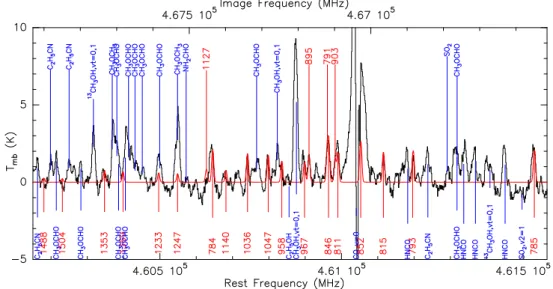
Figure 1.3: APEX observations of the Hot Molecular Core G327.3-0.6 (double-sideband mode), overlaid with a model from myXCLASS for CH3CN,v8=1 (red, the size is 1.5^′′, the temperature 300 K, the line width 4 km/s and the CH3CN column density is 10¹⁷cm⁻²). The energy of the lower level is given in K.

Embedded high-mass stars, whose entire radiation is absorbed by dust and converted to the infrared, can already have developed an Hiiregion, which emits free-free radiation in the radio regime. As their dust emission shows up in the IRAS maps, Wood & Churchwell (1989) searched for ultracompact Hiiregions in color-selected IRAS sources. Due to the clustering of high-mass stars, one can expect to find HMCs close to them. Also, HMCs can be heated by the star(s) in the UCHiiregions, in which case it is considered as external heating, in contrast to heating by internal sources which have not yet developed a UCHiiregion.

Finally, HMCs are often associated with water masers (at 22 GHz), which require several hundred K and>10⁸ cm⁻³ to be excited. Also OH and CH3OH masers occur. Masers are very strong, non-thermal lines which arise from population inversion. They are very compact and easily detectable.

Ouflows also often appear in HMCs, but to definitely detect a hot core, the spectrum has to show many lines from complex organics and highly excited states (e.g. Fig. 1.3).

1.3.2 Chemistry

Chemistry in the ISM differs signifcantly from chemistry on Earth due to the low number densities, which prevent three-body encounters (e.g. Tielens 2005). Therefore, reactions with a single product cannot happen due to energy and momentum conservation. Also the low temperatures typical in molecular clouds (∼10 K) prevent endothermic reactions or reactions with an activation barrier . Instead, charge-transfer reactions between neutral and ion dominate the gas-phase chemistry. A typical sequence of events is the ionization of H2by cosmic rays, the formation of H⁺₂, H⁺₃, and HCO⁺by collisions with H2and CO. Subsequent reaction pathways can lead to larger molecules, which finally recombine with an electron and lose (at least) a hydrogen atom. The products of such gas-phase reactions tend to be rather poor in hydrogen (e.g. carbon-chain molecules).

The majority of molecules in the ISM were found in HMCs, including complex molecules (Herbst & van Dishoeck 2009). With the high temperatures and large densities, gas-phase chemistry in HMCs is somewhat richer than in other molecular environments, in particular activation barriers can be overcome and endothermic reactions can occur. Probably even more important is grain-surface chemistry, as the released binding energy can be given to the dust grain and more reactions are possible. Atoms and molecules stick to the grains when they collide, and ice mantles form at low temperatures. Hydrogen atoms can move on the surface, and at higher temperatures also heavier atoms/molecules can move. This way, the hydrogen atoms scan the grain until they find a reaction partner and form the most abundant molecule H2 (Duley & Williams 1993) as well as saturated molecules such as H2O (water), NH3(ammonia) and CH3OH (methanol).

The astrochemistry of HMCs thus develops from freezing out of molecules to form ice mantles around dust grains in a cold phase, the warm-up with increased mobility and reacitivity and eventual evaporation of the ices when the newly formed stars provide heating, and gas-phase chemistry in a hot phase. Garrod et al. (2008) have simulated the reactions occuring in gradual warm-up of the grain mantles and the gas-phase, leading to varying abundances of the molecules. In principle, such simulations can provide age estimates of HMCs, as chemical timescales are long enough in interstellar conditions and the gas does not reach a chemical equilibrium. However,

(18)

this requires detailed knowledge of the history of collapse and warm-up for different parts of the cores, as well as reliable reaction networks also at high temperatures.

An indication of age could be e.g. the abundances of SO and SO2, as they seem to differ substantially between sources. Sometimes, N- and O-bearing molecules are found at different locations, which could be an age or temperature effect (Rodgers & Charnley 2001). Very complex reaction networks and history determine the abundances of the different molecules, starting from the elemental abundances, which in the solar neighborhood are relative to hydrogen 0.07 (He), 6.8×10⁻⁴(O), 3.7×10⁻⁴(C), 1.2×10⁻⁴(N), and 1.6×10⁻⁵(S) (Cameron 1973).

1.3.3 Physical Structure

The physical structure of HMCs is not well known, and differs from source to source. Most sources have masses on the order of 10³M_⊙, and luminosities on the order of 10⁵L_⊙, which is reprocessed by dust and mostly emitted in the far infrared.

The density reaches values well above 10⁷ H2 cm⁻³in the central region and falls offwith radius. This con- densation of matter is expected from collapse. Some HMCs show fragmentation in the sense of multiple centers.

It is not clear how to define the size for a continuous density distribution; the area where most of the dust and line emission is concentrated (if observed with an interferometer) is typically on the order of 0.1 pc.

The temperature is higher in the inner part than further outside. This temperature gradient points to internal heating by the formation of embedded stars or protostars. Average temperatures, deduced from line ratios, are 100–300 K, but probably all temperatures up to the dust sublimation temperature of around 1500 K are present on small scales.

Apart from turbulence, which is imprinted in the line widths, there are many indications for systematic motions such as outflows, rotation, and collapse. Velocity gradients seen at high spatial resolution can be interpreted as rotating massive disks or toroids (Beltr´an et al. 2005, 2011; Zapata et al. 2010). Outflows can be observed on larger scales and in high-velocity line wings. Simultaneous infall often shows up in asymmetric line profiles or in red-shifted absorption (e.g. Qiu et al. 2011; Furuya et al. 2011).

1.3.4 Sources

A few dozen sources are currently known in the Galaxy, and they display a high individuality. The sources investigated in this thesis are briefly described in Chapter 3, as they were all observed with the APEX telescope (Table 3.1). These are G10.47+0.03 (Sect. 3.8.1), IRAS 16065-5158 (Sect. 3.8.2), G327.3-0.6 (Sect. 3.8.3), G34.26+0.15 (Sect. 3.8.4), G31.41+0.31 (Sect. 3.8.5), IRAS 12326-6245 (Sect. 3.8.6) , IRAS 17233-3606 (Sect. 3.8.7), NGC6334-I (Sect. 3.8.8), W51e (Sect. 3.8.9), W51d (Sect. 3.8.10), SgrB2-M (Sect. 3.8.11), and SgrB2-N (Sect. 3.8.12).

SgrB2-M was also observed with Herschel (Chapter 4), and G10.47+0.03, SgrB2-M and -N with the VLA (Chapter 5) and the SMA (G10.47+0.03 in Chapter 6, continuum of SgrB2 in Chapter 7). They are all extremely massive HMCs associated with HCHiiregions.

Among the other HMCs, Orion-KL is the most prominent source with a distance of only 414 pc (Menten et al.

2007). It could be an unusual hot core though, heated by a nearby explosive event rather than internal high-mass stars (Zapata et al. 2009b, 2011).

1.4 Problems

The understanding of high-mass star formation and of astrochemistry has to face several problems in theory, observations, and analysis. Some of them are described in the following.

1.4.1 Theory

Although much progress has been made in the last years, it is still not well understood how high-mass stars form.

Examples of problems include the relative contribution of different forms of pressure to the support against gravity, the exact ways of collapse and accretion, and the effects of feedback.

High-mass stars form only in clusters (Lada & Lada 2003) and usually in multiple systems, while low-mass star formation can also occur in relative isolation. Furthermore, they are concentrated in cluster centers (mass segregation), and it is under debate if they formed there or have migrated there due to dynamical interactions.

Apart from that, the stellar initial mass function seems to be very universal, and the core mass function follows a similar slope. It is not clear what regulates the IMF, and what the connection to the core mass function is.

(Magneto-)hydrodynamical simulations of the star formation process can hardly include all the physics that is involved (e.g. detailed time-dependent heating/cooling), and lack the resolution to handle all relevant structures due to limited computing power. The latter hurdle is bypassed by sink particles, which form ad-hoc stars once

(19)

1.4. PROBLEMS 17

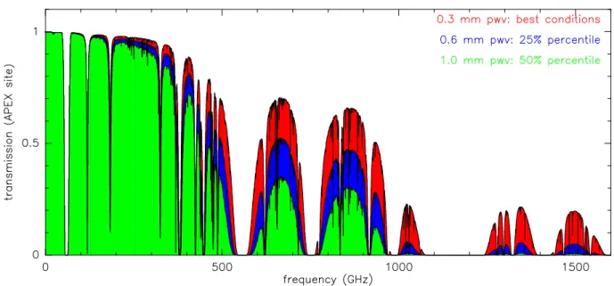
Figure 1.4: Atmospheric transmission at the APEX site, for columns of precipitated water vapor of 0.3, 0.6 and 1 mm (courtesy: P. Schilke).

the density gets too high. Still, even if the evolution is computed correctly, the outcome depends on the initial conditions, which have to be set a priori. It is not yet possible to compute several models, since one run takes several months to complete on the best available computers.

Astrochemical calculations need a complete network of reaction rates, as well as dust properties and time- dependent physical conditions. The latter could come from hydrodynamical simulations.

1.4.2 Observations

High-mass stars are rare and undergo a fast formation and evolution process. Therefore, not many in a given stage of formation are present in the Galaxy, and they are mostly far away.

Moreover, the structures are very compact, and the cores from individual stars overlap due to the strong clustering of high-mass stars. Hence, very good angular resolution is a critical issue.

Due to the large dust column densities and the frequency-dependent dust opacity, most of the sources are obscured at short wavelengths. In the optical and infrared, one can only see a cold surface, while the hot core is hidden and only visible at submillimeter and radio wavelengths. These in turn are partly obscured by the Earth’s atmosphere, in particular by water vapor. The transparency depends on weather and location. Figure 1.4 shows the transparency of the atmosphere as function of observing frequency for one of the best sites, under different weather conditions.

1.4.3 Analysis

The extreme richness of spectral lines that HMCs exhibit leads to spectral confusion and blending, i.e. line overlap.

While this is less of a problem for strong lines (e.g. from simple molecules that have only relatively few transitions), it makes the detection of complex molecules, which have many weak transitions, very difficult and in many cases impossible, regardless of sensitivity. But also in the analysis of profiles of strong lines one has to be aware of possible blending by neighboring lines.

The individuality of the sources impedes a comparison to simulations, which have necessarily different initial conditions. This makes it difficult to test theories, which lack clear observational predictions.

The observed radiation depends on the physical structure, and it is not straightforward to derive physical and chemical quantities such as temperature, density, and molecular abundances. The abundances can vary with physical conditions, which renders the problem even more difficult.

For a proper analysis of the observations, one needs radiative transfer modeling. The models should be as simple as possible to allow a combination of parameters to reproduce the observations. Defining parameters and scanning the parameter space for solutions poses a giant challenge.

The modeling needs physical inputs, many of which are very uncertain or not yet measured or calculated.

(20)

These include dust opacities, collision rates of molecules (collected at the database LAMDA²and BASECOL³), and line frequencies (collected at the databases CDMS⁴and JPL⁵).

1.5 Aims

The aim of this thesis is to constrain the structure of HMCs (their density, temperature, velocity, and abundance distribution) in order to facilitate future progress in high-mass star formation and in astrochemistry. This shall be achieved by exploring four ground-breaking techniques, two on the observational and two on the analytical side.

1.5.1 High Submillimeter Frequencies

High submillimeter frequencies (>600 GHz) are challenging due to atmospheric absorption (Fig. 1.4) and receiver technology. New instruments, namely APEX, the SMA, and Herschel, open up these frequency windows and provide the opportunity to use them in my research (Chapters 3, 4, and 6). Compared to lower frequencies, rotational transitions trace higher energy levels and the larger dust opacity facilitates absorption features, which are sensitive probes of the source structure. Also the continuum gives hints on the structure, as dust becomes optically thick.

1.5.2 High Resolution

High angular resolution requires a large aperture D, because the beam size (FWHM) is 252^′′^λ[mm]_D[m]. As the wavelength λ has to be long enough to penetrate the foreground dust, this means interferometers (see Sect. 2.5).

Currently the best possible resolution provides the VLA in its most extended configuration and at its shortest wavelength (7 mm, Chapter 5). However, the brightness sensitivity decreases with higher resolution. At shorter wavelengths, where the dust emits stronger, the SMA can be used (Chapter 6). Spectral resolution is essential to measure line shapes, a resolution of around 1 km/s is sufficient and provided by the heterodyne receivers.

1.5.3 Modeling Line Shapes

Not only the intensity of spectral lines contain important information, but lines have different optical depths at different velocities (frequency offsets from the rest frequency). While optically thin lines have usually a Gaussian shape, optically thick lines trace different parts of the source at different velocities. This offers access to the line-of- sight structure such as the excitation temperature profile and the velocity field (systematic motions like outflows, rotation, and infall) and can even constrain sub-beam size structures by detailed radiative transfer modeling, e.g.

with RATRAN (Chapters 3 and 4).

1.5.4 Three-dimensional Modeling

Although models should be as simple as possible to reproduce the observations, real sources are not that simple.

In particular, as high-resolution maps show, multiple cores and stars have formed, so spherical or cylindrical symmetry does not apply. Instead, one has to go for true three-dimensional models, at best in combination with computation of the dust temperature. This can be done with RADMC-3D (Chapters 5 and 6).

2http://www.strw.leidenuniv.nl/˜moldata

3http://basecol.obspm.fr

4http://www.cdms.de

5http://spec.jpl.nasa.gov

(21)

Chapter 2

Radiative Transfer

This chapter starts with brief descriptions of molecular energy levels and radiative transitions between them (Sects. 2.1 and 2.2). The determination of the level populations is discussed in Sect. 2.3. Section 2.4 deals with the resulting radiation. These sections are based on my diploma thesis (Rolffs 2007), and illustrated with examples from the HCN molecule¹, which plays an important role in this thesis. The radiative transfer theory is also described e.g. in Rybicki & Lightman (1979), Genzel (1991), and Rohlfs & Wilson (2004).

How to measure the radiation with single-dish and interferometric telescopes is described in Sect. 2.5. Radiative transfer modeling is discussed in Sect. 2.6.

2.1 Molecular Energy Levels

2.1.1 Rotational Levels

The rotational energy of molecules has discrete levels due to the quantization of angular momentum L (e.g. Haken

& Wolf 2003). For linear molecules, it is given by E_rot= L²

2Θ = h²

8π²ΘJ(J+1) (2.1)

with the moment of inertiaΘ = Pm_iR²_i (m being the mass of a nucleus and R its distance from the center of mass). J is the quantum number of angular momentum. Its projection onto an arbitrary direction is another quantum number, whose possible values are J,J−1, ...−J. These 2J+1 projections have the same energy, so the energy level is degenerate and its statistical weight is 2J+1.

Θdepends on the equilibrium distances of the nuclei. These can be distorted by rotation or vibration. Due to centrifugal forces, R and thusΘincreases with rotation, so high-J states have a somewhat lower energy than they would have for constantΘ. Including this effect, the energy levels can be approximated by Erot = BJ(J +1)− D(J(J+1))²with the molecular constants B and D. Substituting one nucleus with a heavier isotope changesΘand hence the rotational energy levels.

2.1.2 Vibrational Levels

Vibrational levels have higher energies than pure rotational levels. According to quantum mechanics, a harmonic oscillator has a vibrational energy proportional to (v+¹₂). v is the vibrational quantum number, and even for v=0 there are fluctuations which cause a substantial minimum vibrational energy (as the molecule cannot go lower in energy, it can be set to zero in practice). The proportionality constant depends on the force gradient and the (reduced) mass. For an anharmonic oscillator, a term proportional to (v+¹₂)²and to the inverse of the dissociation energy has to be subtracted.

Different modes of vibration can be distinguished. Stretching vibrations are periodic changes of the bonding length, while bending vibrations change the angles between the bonds. The latter occur only for molecules with more than two atoms and usually require less energy. The energies depend on the atomic masses and the bonding length. Anℓ-type finestructure arises due to the vibrational deformation of the molecule and the coupling between vibration and rotation.

1On Earth, HCN (hydrogen cyanide) is known as hydrocyanic or prussic acid (in German Blaus¨aure) when it is dissolved in water. It is very poisonous: by reacting with iron of a certain enzyme, it blocks the respiration mechanism of cells and prevents the incorporation of oxygen from the blood. For prebiotic chemistry, it is important as a building block of amino acids.

19

(22)

Electronic levels (the excitation of electrons) are generally so high in energy that they are not excited in star- forming regions.

2.1.3 Example: HCN Levels

The molecular constants that describe the rotation of HCN are B=1.478222 cm⁻¹ =2.127 K=44.316 GHz²and D=2.91×10⁻⁶cm⁻¹ =4.2×10⁻⁶K=87.2 kHz. As the quadrupole moment of the¹⁴N nucleus couples to the gradient of the electric field, a hyperfine splitting of the energy levels occurs. This is important only for the lowest rotational states. The 1–0 transition is split into 3 lines which differ by 3.5 MHz (12 km s⁻¹), while the six 4–3 transitions are distributed over 3 km s⁻¹, with 95% of the line strength in the central transitions.

Vibrational modes of HCN are stretching of the C-N or the C-H bonds and bending of the C atom perpendicular to the NH line. The energy of the C-H stretch vibrational mode is about v1×4764 K (the quantum number v1denotes the number of quanta in this mode), the C-N stretch mode has v3×3017 K (less than CH due to the higher reduced mass). The designation (1 or 3) is sometimes reversed. Bending vibrations require v2×1027 K.

While the stretching vibrations keep the linear structure of the molecule, the bending vibrations can occur in the plane of rotation or perpendicular to it, so the bending mode is actually split into two, slightly different modes.

If the orientation of each of the v₂quanta is+or−, the sum is the quantum numberℓ, which therefore goes from v2to−v2in steps of 2.ℓcouples rotation and vibration, and is actually another rotational quantum number: Due to the bending deformation, rotation around the axis becomes possible. The result of the two simultaneous rotations is that J cannot be smaller thanℓand that a bending mode of quantum number v2splits into v2+1 levels, whose energies depend mainly on the absolute value ofℓand slightly on its sign (the direction of rotation), which is (−1)^J for the lower levels. An alternative designation is e for the lower levels (and the ground vibrational state) and f for the upper levels.

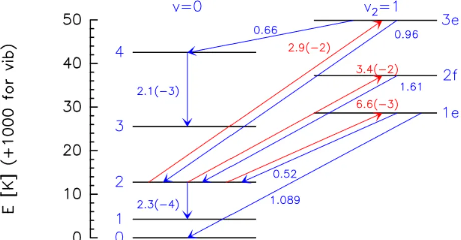
The energy level diagram of HCN is summarized in Figure 2.1 (based on Maki 1974; Maki et al. 2000).

2.2 Radiative Transitions

2.2.1 Einstein Coefficients

The probabilities for radiative transitions are described by the Einstein Coefficients (Einstein 1916). Considering two levels, the populations nuand nl(number densities of upper and lower level, respectively) change according to

dn_u dt =−dn_l

dt =−Aulnu−BulJulnu+BluJulnl (2.2) nucan decrease by spontaneous emission, which is proportional to nuitself and to the A coefficient. The B coeffi- cients describe transitions induced by radiation. The probabilities are proportional to the mean intensity Jul, which is the intensity from all directions weighted by the profile functionΦ(Sect. 2.4.4; it is centered atνul = Êû⁻_hÊ^l, where E denotes the energy), Jul =R _dΩ

4π

R dνIΦ. Induced emission, described by the second term, means that a passing photon of the right frequency is doubled. This process is thus proportional to nu. The last term describes the absorption of a passing photon, which causes the transition from the lower to the upper level.

The Einstein B coefficients are proportional to the A coefficient (Sect. 2.3.2). The strength (Einstein A coeffi- cient) of a transition is calculated quantum-mechanically from the wave functions of the two states. For electric dipole transitions, it is proportional toµ²ν³with the dipole momentµ. For forbidden (multipole) transitions, it is very low. Hence, radiative transitions are unlikely if they violate certain selection rules, and are more likely the larger the energy gap is. The selection rules describe the conditions for allowed (strong) transitions. For instance,

∆J=1 is necessary for a rotational transition, since the photon carries one quantum of angular momentum.

2.2.2 Example: HCN Transitions

Due to the corresponding energy gaps, directℓ-type transitions occur in the radio regime, rotational transitions in the mm to far-infrared regime, vibrational transitions in the infrared (14µm for∆v2=1) and electronic transitions in the ultraviolet (190 nm for the electronic state of HCN).

The selection rules are bit more complicated when the vibrational levels are included. Pure rotational transitions stay within a certain vibrational state. Rovibrational transitions (which change the vibrational state) require∆J=1 for the lower level of anℓ-type doublet and∆J =0 for the upper level. Directℓ-type transitions are not electric dipole transitions and hence weak. They exchange upper and lower level of the same J with∆ℓ=2.

2All units denote the energy, making use of E=kT=hν=^hc_λ

(23)

2.2. RADIATIVE TRANSITIONS 21

Figure 2.1: Energy levels of HCN. The left panel shows the vibrational levels, the central panel the lowest rota- tional levels and the right panel shows levels of the first vibrational state. Some transitions with their Einstein A coefficient (numbers in parenthesis are powers of 10) are indicated.