Globalisation, Domestic Political Institutions, and Cli- mate Commitment and Performance
Annex
Dissertation zur Erlangung des Doktorgrads an der Fakultät für Philosophie, Kunst-, Geschichts- und Gesellschaftswissenschaf-
ten der Universität Regensburg
Vorgelegt von Romy Escher geb. in Ludwigsburg
Regensburg 2020
Table of Contents
A6 Research design 4
A6.1 Developed country sample 4
A6.2 Measurement of ideology heterogeneity among veto players 6 A6.3 Validity and reliability of measurement approaches of
political corruption 8
A6.4 Validity and reliability of measurement approaches of
vertical accountability 10
A6.5 Validity and reliability of measurement approaches of
horizontal accountability 11
A6.6 Validity and reliability of measurement approaches of
civil rights 12
A6.7 Validity and reliability of measurement approaches of types of
autocracy 14
A7 Climate commitment 19
A7.1 Univariate statistics 19
A7.2 Bivariate correlations 20
A7.3 UNFCCC ratification 25
A7.4 Kyoto Protocol ratification 37
A7.5 Analysis of the model assumptions 48
A7.5.1 Model fit 48
A7.5.2 Test of the model assumptions 49
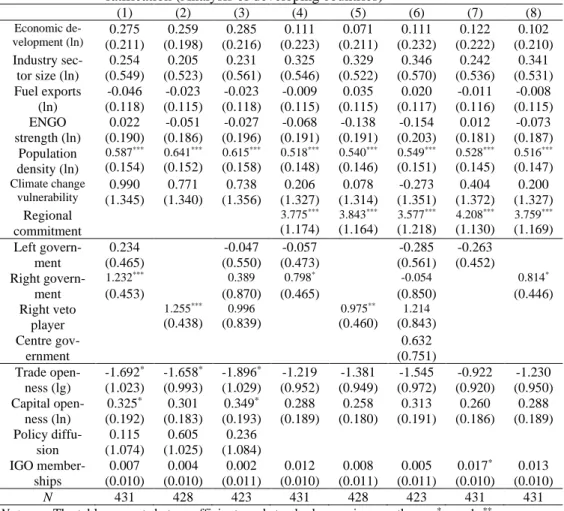
A7.6 Robustness analysis 60
A8 Climate performance 62
A8.1 Analysis of the model assumptions of TSCS 62
A8.2 Developed countries 66
A8.2.1 Univariate statistics 66
A8.2.2 Bivariate correlations 68
A8.2.3 Additive effects of international integration: Regression tables 71
A8.2.4 Analysis of the model assumptions 90
A8.2.5 Robustness analysis 90
A8.3 Developing countries 96
A8.3.1 Univariate Statistics 96
A8.3.2 Bivariate correlations 97
A8.3.3 Globalisation, domestic political institutions and climate
performance 101
A8.3.4 Analysis of model assumptions 108
A8.3.5 Robustness analysis 110
A6 Research design
A6.1 Developed country sample
Table A6.1 presents countries that are Annex I parties of the UNFCCC. It illustrates that post-communist countries as defined by McCormick (2001) are classified by the UNFCCC as economies in transition. Moreover, not all Annex I countries are classified as developed countries based on the World Bank criteria (high-income country). In my analysis of developed countries, I focused on Annex I countries that are classified as high-income and having a population of at least 500,000 individu- als. High-income countries that are not Annex I parties to the climate treaty include Andorra, Antigua and Barbuda, The Bahamas, Bahrain, Barbados, Brunei Darus- salam, Israel, Kuwait, Puerto Rico, Qatar, San Marino, Saudi Arabia, Seychelles, Singapore, South Korea, St. Kitts and Nevis, Trinidad and Tobago as well as the United Arab Emirates. Furthermore, states with missing data for independent and dependent variables were not included. Bold printed countries in Table A6.1 were selected. The table reveals that my developed country sample is a homogeneous group of established democracies that are all classified by McCormick (2001) as liberal democracies.
Table A6.1 Annex I Countries
Country EiT HIE LD NIC Post-C <500,000 No Data
Australia X X
Austria X X
Belarus X X
Belgium X X
Bulgaria X X
Canada X X
Croatia X X
Cyprus X X X
Czech Re- public
X X X
Denmark X X
Estonia X X
Finland X X
France X X
Germany X X
Greece X X
Hungary X X
Iceland X X X
Ireland X X
Italy X X
Japan X X
Notes: Source: UNFCCC (2014); EiT = Economies in transition (UNFCCC 2014); HIE = High-income economy in 2005 (GNI per capita >=10.725) World Bank; LD = Lib- eral democracy (McCormick 2001); NIC = Newly industrializing country (McCor- mick 2001); Post-C= Post-communist country (McCormick 2001); < 500,000 = Population size during the research period is below 500,000 citizens; No data = Data on independent and/or dependent variables is completely missing. Bold printed countries are selected for my analysis of developed countries.
Table A6.1 Annex I Countries (continuation)
Country EiT HIE LD NIC Post-C <500,000 No Data
Latvia X X
Liechten- stein
X X X
Lithuania X X
Luxembourg X X X
Malta X X X
Monaco X X X
Netherlands X X
New Zea- land
X X
Norway X X
Poland X X
Portugal X X
Romania X X
Russian Fed- eration
X X
Slovakia X X X
Slovenia X X X
Spain X X
Sweden X X
Switzerland X X
Turkey X
Ukraine X X
UK X X
USA X X
Notes: Source: UNFCCC (2014); EiT = Economies in transition (UNFCCC, 2014); HIE
= High-income economy in 2005 (GNI per capita >=10.725) World Bank; LD = Liberal democracy (McCormick, 2001); NIC = Newly industrializing country (McCormick, 2001); Post-C= Post-communist country (McCormick, 2001); <
500,000 = Population size during the research period is below 500,000 citizens; No data = Data on independent and/or dependent variables is completely missing.
Bold printed countries are selected for my analysis of developed countries.
A6.2 Measurement of ideology heterogeneity among veto players
This section examines the political constraints variables from Henisz (2002) to es- tablish to what extent these measures are valid and reliable measures of ideological heterogeneity among veto players. As political constraints, Henisz (2002, 2000) considers the number of veto players in the governmental system, the policy pref- erences of veto players and the preference coherence of legislative veto players (Henisz, 2002, p. 380). He provides two measures: POLCON3 and POLCON5.
While POLCON3 counts the executive, the lower house and the upper house as institutional veto players, POLCON5 additionally includes federalism and judiciary (Henisz, 2002, p. 380). The executive is treated as present in all political systems
(Henisz, 2000, p. 27). Henisz (2002) assumes a unidimensional policy-space of pol- icy preferences of veto players. Regarding concept specification, POLCON5 is overly maximalist (Jahn, 2010, p. 57). It considers with the judiciary a veto player that is not always relevant for policy outputs (Tsebelis, 2002, p. 205). POLCON3 is overly minimalistic (Jahn, 2010, p. 57). It neglects to count the president as a po- tential veto player. Regarding concept logic, Henisz (2002) counts both bicameral- ism and federalism as separate veto players (redundancy) (see Chapters 4 and 5; see also Jahn, 2010, p. 54; Tsebelis, 2002, p. 205). In accordance with the veto player concept, both measures consider the policy preferences of veto players as well as the absorption rule by counting only veto players that are not redundant regarding their party composition. Henisz's (2002) conceptualisation, however, is a mixture of the veto player and veto point concept. The number and preferences of veto play- ers are weighted equally.
To consider the absorption rule, Henisz (2002) compares the partisan composition of the executive with each legislative chamber. However, he only considers the names of the political parties. These names change over time within his dataset.
Because of data availability and comparability, Henisz (2000, p. 5; Henisz, 2002, p.
380) uses estimated preferences. He assumes that preferences of veto players are distributed randomly around the status quo (Henisz, 2002, p. 380; see also Henisz, 2000, p. 5). He defines the utility of each veto player from a policy x as |x-xI|. The assumption that all preference orderings have the same likelihood enables him to estimate preferences using a spatial model of political interaction (Henisz, 2002, p.
363; Henisz, 2000, p. 6). In the case of neither completely aligned nor completely independent legislative veto players from the executive, the index considers prefer- ence cohesion of legislative veto players (Henisz, 2002, pp. 364, 383). For this pur- pose, he weights legislative veto players with the partisan fractionalisation of the total legislative chamber (number of all parties in parliament) (Tsebelis, 2002, p.
205). The indicators of potential legislative veto players are problematic. For in- stance, he does not regard the German Bundesrat as potential veto player. Secondly, POLCON3 and POLCON5 are based on estimated instead of empirically observed policy preferences (Jahn, 2010, p. 59). Third, the indicator of cohesion of legislative veto players does not measure internal cohesion of collective veto players (Jahn, 2010, p. 55; Tsebelis, 2002, p. 205). Henisz (2002) provides his disaggregated data for further research online (replication).
Henisz's (2002, p. 380) political constraints measures result from the subtraction of the level of political discretion from 1. The level of political discretion is ‘the ex- pected range of policies for which all political actors with veto power can agree upon a change in the status quo’ (Henisz, 2002, p. 380f.). Based on his assumptions, he proposes that the difference between randomly distributed preferences of two veto players is 1/(n+2) (n= number of actors) (Henisz, 2002, p. 381; Henisz, 2000, p. 6). In the case of two veto players, six possible preference orderings are possible (Henisz, 2002, p. 381). Consequently, POLCON3 and POLCON5 result from the average of the political constraints measures regarding the possible preference or- derings (Henisz, 2002, p. 382). While this aggregation rule fits the veto player con- cept (Jahn, 2010, p. 55), it measures only the average expected distance between veto players. Moreover, he weights the average distance between veto player with
the fractionalisation of legislative veto players. Thus, variation in the Henisz (2002) measures within countries and between countries results only from different num- bers of veto players and political parties in the upper and lower chambers. Jahn (2010, p. 55) concludes that ‘[i]t remains unclear though what this dimension is intended to represent.’ Replicability is given in the case of the political constraint's measures.
To conclude, the underlying concept of Henisz (2002) differs considerably from Tsebelis's (2002) veto player approach. Both measures show validity and reliability problems in the three phases of index construction. Finally, in contrast with the as- sumptions of veto player theory, variation on Henisz's measures results from the number of veto points and the fractionalisation of legislative chambers.
A6.3 Validity and reliability of measurement approaches of political cor- ruption
This section outlines that both the political corruption index (CPI) from Transpar- ency International and the control of corruption measure from the World Govern- ance Indicators (WGI) (Kaufmann et al., 2010) have validity and reliability prob- lems in all three phases of index construction. They are frequently used in cross- national research.
Conceptualisation. Both measures intend not to capture political corruption itself but public perceptions of political corruption. The CPI further limits its concept to public sector corruption as it focuses on public perceptions of corrupt behaviour within the public sector (Transparency International 2016b, no page number). It does not define public sector corruption. Kaufmann et al. (2010) do not specify their concept beyond a short definition of political corruption. The relationships among the elements of political corruption and their relative importance remain unclear.
The CPI additionally does not specify its underlying concept and differentiate it from related concepts. Moreover, the underlying concepts of both the CPI and the World Bank indicator have changed over time (Knack, 2006, p. 18).
Measurement. The methodological literature suggests that the reliability of compo- site measures is increased by the use of multiple data sources. The CPI and the WGI both have the advantage of relying on multiple data sources (McMann et al., 2016, p. 13; Transparency International, 2016b, no page number). The former summarises data from independent research institutions and business information (Transparency International, 2016b, no page number); the latter is based on indicators from re- search institutes, international and domestic governmental institutions and interna- tional surveys from the business sector (The World Bank Group, 2019b). Both measures also consider multiple data types. The CPI summarises survey data and expert evaluations (Transparency International 2016b, no page number). The con- trol of corruption measure includes survey data of households and firms; data from expert evaluations; data from commercial business information providers and non- governmental institutions; and information from public international and domestic institutions (Kaufmann et al., 2010, p. 5; The World Bank Group, 2019b, 2017).
The WGI corruption measure considers indicators of different forms of corrupt be- haviour of the government, the legislative branch, the judicial branch, public offi- cials, political parties and the media (The World Bank Group, 2019b). With the
inclusion of indicators of corrupt behaviour of non-political actors and its institu- tions, the WGI corruption measurement refers to a broader definition of political corruption than its conceptualisation. In addition, it is based on indicators of other concepts, such as political trust (trust in politicians). Finally, Treisman (2007, p.
215) notes that the control of corruption measure summarises indicators of different types of corruption and different characteristics of corruption (frequency, severity).
He finds it is unclear what it measures (Treisman, 2007, p. 215). In comparison to the conceptualisation of the CPI, Transparency International considers data on pub- lic sector and private sector corruption (McMann et al., 2016, p. 9).
The CPI includes only country-years for which at least three data sources are avail- able (Transparency International, 2016a, p. 4). However, its values are only com- parable over time since 2012 (Transparency International, 2016a, p.1; Transparency International, 2016b, p. 2). Data sources changed again in 2016 (Transparency In- ternational, 2016b, p. 2). An additional problem of the CPI is that it uses the same data in several country-years (Treisman, 2007, p. 217). The WGI include most countries but are only available for few country-years from to 1997-2015. Moreo- ver, the indicators are not comparable over time. This stems from the variation of data sources over time, the inclusion of additional data and changes in the weights to aggregate the data sources (Kaufmann et al., 2010, p. 6; The World Bank Group, 2017). Moreover, not all data sources are available for all countries (The World Bank Group, 2017).
To conclude, while both measures consider multiple data sources and data types, both measures consider indicators that do not fit their underlying concepts and both are not comparable over time.
Aggregation. Transparency International first standardises the indicators using a z- transformation re-scaled to a scale from 0 to 100 and then aggregated using the mean (Transparency International, 2016a, p. 2f.). The WGI authors standardise the indicators and averages indicators that measure the same concept (Kaufmann et al., 2010, p. 2). They then aggregate these indicators using a weighted average (Kauf- mann et al., 2010, p. 2). For this purpose, they use an unobserved components model (Kaufmann et al., 2010, p. 9). Kaufmann et al. (2010) assume that the global average of their corruption measure is constant over time. Consequently, their corruption measure cannot be used to analyse country trends over time (Kaufmann et al., 2010, p. 12). Knack (2006, p. 18) argues that the CPI and the WGI measures are not trans- parent regarding their weighting. The WGI authors additionally publishes most of the indicators of their composite indices (Kaufmann et al., 2010, p. 7). In sum, both measures show validity problems in the aggregation phase.
To conclude, while the CPI and the Control of Corruption indicators from the WGI have the advantage of multiple data types and data sources, they show considerable validity problems as indicators of political corruption in all three measurement phases. Crucially, they do not measure political corruption but public perceptions of corruption. The WGI index is additionally broader than the political corruption concept in its measurement.
A6.4 Validity and reliability of measurement approaches of vertical ac- countability
Besides the Vertical Accountability Index, the political rights measure from Free- dom House and the index of democratisation from Vanhanen (no year) offer world- wide panel data on vertical accountability. This section shows that both have valid- ity and reliability problems as indicators of vertical accountability.
Conceptualisation. The authors of Freedom House neither specify their concept nor differentiate it from related concepts. Freedom House understands political rights as political participation rights (Pickel & Pickel, 2006, p. 210). Beyond this defini- tion, the underlying concept of the Freedom House measure is not explained (and there is no transparency). Secondly, based on the four categories of their indicators, it is not parsimonious. While the authors consider all relevant elements of vertical accountability—universal active suffrage, universal passive right to vote, free and fair elections, and elected political representatives (Merkel, 2016, p. 261; Merkel, 2004, p. 38, 42)—they also include elements of related concepts, for example, gov- ernment corruption. Regarding concept logic, Freedom House does not address the vertical and horizontal relationships between the elements of its concept. Following Dahl, Vanhanen (no year) defines democracy as participation and contestation. Both dimensions are regarded as necessary conditions of democracy. His concept had variable performance with regard to its validity in the conceptualisation phase. On the one hand, it is transparent, applicable worldwide and distinguished from related concepts; it also shows no problems with regard to conflation and redundancy. On the other hand, it neglects relevant elements of vertical accountability. Its underly- ing concept is only partially coherent. It specifies the horizontal relationship be- tween participation and competition, but it neither identifies sub-components nor specifies their horizontal and vertical relationships.
Measurement. The Freedom House measures each subcategory by 10 indicators (Freedom House, 2017, no page number). The first category consists of items that measure whether political authorities are elected in free and fair elections. The sec- ond category includes items that measure the opportunity of citizens to organise and participate in parties, the possibility that the opposition takes over, the independence of citizens’ votes from the influence of powerful groups and active suffrage of dif- ferent social groups. The final category encompasses items that measure the author- ity of the freely elected government, corruption, and vertical accountability between elections. Their measure additionally evaluates traditional monarchies and unequal treatment of ethnic groups by the government (Freedom House, 2017, no page num- ber). Each indicator is coded on a scale from 0 to 4 by experts, including native coders based on multiple sources from the media, science, NGOs, and professionals (Freedom House, 2017, no page number; Pickel & Pickel, 2006, p. 211). The Free- dom House Political Rights index shows deficits regarding validity. Several indica- tors—for example, ‘Is the government free from pervasive corruption?'—do not measure aspects of vertical accountability. Some indicators are not unidimensional (Lauth & Kauff, 2012, p. 11). Finally, the measurement level is not explained. Free- dom House does not provide coding criteria (Pickel & Pickel, 2006, p. 219). While Freedom House provides annual values for nearly all countries, the comparability
over time is limited as the methodology has changed over time (Freedom House, 2017, no page number; see also Pickel & Pickel, 2006, p. 219). Disaggregated data is only available for the most recent years.
The competition indicator from Vanhanen’s index (Vanhanen, no year) results from the subtraction from 100 of the percentage of votes for the largest party in parlia- mentary elections, or alternatively, the subtraction from 100 of the percentage of votes for the successful candidate in presidential elections. Participation is meas- ured by the percentage of citizens of the total population that participated in the last national election. In semi-presidential systems, Vanhanen considers both and weighs them based on their importance. Vanhanen's indicators are reliable. They are based on statistical data. The estimation rule is constant across countries and over time. Both indicators are available for nearly all countries worldwide and cover my entire research period. In contrast, the content validity for both indicators is questionable. It does not capture the overall concept of vertical accountability. It neglects restrictions on opposition parties and their independence from the ruling party. The validity of the participation indicator is restricted as it is dependent on demographic developments (Pickel & Pickel, 2006, p. 197). Vanhanen (no year) neglects to consider active suffrage and to what extent elections are free and fair.
Moreover, he at most indirectly considers whether the chief of executive is elected.
The competition indicator does not consider the difference between elections sys- tems—such as majority or proportional vote (e.g., Pickel & Pickel, 2006, p. 197).
Aggregation. The index of democratisation performs well in aggregation. It results from the multiplication of the participation and competition indicators. This aggre- gation rule fits Vanhanen’s assumption that both dimensions are of equal im- portance and necessary conditions of democracy. The political rights measure is an additive index. The aggregation rule and weighting are not explained.
In sum, the Freedom House Political Rights index, as well as the index of democ- ratisation, show considerable validity and reliability problems as indicators of ver- tical accountability. This applies to all three phases of index construction for the Freedom House measure and to the conceptualisation and measurement phase for the index of democratisation. While the concept of the former is overly maximalist, the latter neglects relevant elements of vertical accountability. Indicators from both measurements exhibit problems with regard to content validity and comparability over time. The aggregation rule of the political rights measure is not explained.
A6.5 Validity and reliability of measurement approaches of horizontal ac- countability
This section explains why the executive constraints (EXCONST) indicator from Pol- ity IV has not been used to measure horizontal accountability. It captures ‘the extent of institutionalised constraints on the decision-making powers of chief executives’
(Marshall et al., 2016, p. 24) by so-called ‘accountability groups’ (Marshall et al., 2016, p. 24). From this definition, it follows that EXCONST focuses on constraints on the executive that are outlined in the constitution (that is, rules in law vs. rules in use). It captures constraints by the legislative branch, the judicial branch in de- mocracies and ruling parties, important advisers or councils, and the military in au- tocracies (‘accountability groups’) (Marshall et al., 2016, pp. 24f.). Marshall et al.
(2016) assume that autocratic governments, similar to their democratic counter- parts, differ in the extent of constraints that limit their behaviour (Marshall et al., 2016, p. 62). From the perspective of the horizontal accountability concept, the un- derlying concept of EXCONST is characterised by conflation (see also Lührmann et al., 2017, p. 10). It includes ‘non-democratic forms of constraints such as the ruling party in a one-party state or a powerful military’ (Lührmann et al., 2017, p. 10).
Polity IV acknowledges this difference between its measurement concept and the horizontal accountability concept (Marshall et al., 2016, p. 62). Simultaneously, it neglects forms of checks and balances in semi-presidential and parliamentary sys- tems as it evaluates executive constraints from the perspective of the US presidential system (Pickel & Pickel, 2006, p. 191). The data from Polity IV rests on expert evaluations based on multiple sources. The executive constraints measure is solely based on one indicator. Experts code the extent of institutional constraints on the executive on a scale from 1—'unlimited authority' of the executive—to 7— 'execu- tive parity or subordination of the executive—relative to accountability groups (Marshall et al., 2016, pp. 62, 24f.). In accordance with its concept, it considers non- democratic accountability groups. The measurement level is not explained. It does not consider rules in use. The data is comparable across countries and over time. In sum, the underlying concept of the EXCONST indicator and its measurement is characterised by conflation. The reliance on a single indicator in its measurement restricts its reliability and validity.
A6.6 Validity and reliability of measurement approaches of civil rights The Freedom House civil liberties measure and the rule of law index of the WGI both exhibit validity and reliability problems as indicators of civil rights.
Conceptualisation. The Freedom House civil liberties measure and the rule of law indicator from the World Governance indicators show problems in concept specifi- cation and logic. Freedom House defines civil liberties as the protection of the in- dividual from the state (Pickel & Pickel, 2006, p. 210). It does not provide a de- scription of their concept (no transparency). In their measurement, they distinguish four subcategories of civil liberties: freedom of expression and belief, associational and organisational rights; rule of law; and personal autonomy and individual rights (Freedom House, 2017, no year). This means that the underlying concept considers also political rights. It is, therefore, unsuitable for the separate analysis of the sepa- rate effect of civil rights. The rule of law indicator from the WGI aims to measure 'perceptions of the extent to which agents have confidence in and abide by the rules of society, and in particular of contract enforcement, the policy and the courts, as well as the likelihood of crime and violence' (The World Bank Group, 2019a, no page number). A further specification of its underlying concept is not available.
While this definition includes with rule of law some elements of civil rights, it omits other elements and identifies elements that do not fit the common understanding of the rule of law concept (Thomas, 2010, p. 40) (for example, likelihood of crime and violence). In sum, it neglects relevant aspects of civil rights and is not clearly dif- ferentiated from related concepts. Furthermore, the World Governance indicator does not address the relationship between the elements within its concept. Finally, its underlying concept has changed over time (Thomas, 2010, p. 36). Before 2008,
it was supposed to measure the extent of rule of law itself and not perceptions (Thomas, 2010, p. 36).
Measurement. As has been explained above, the political rights and civil liberties measures from Freedom House are based on expert evaluations. Four subcategories of civil rights are identified, and each is measured by multiple indicators: freedom of expression and belief, associational and organisational rights, rule of law, and personal autonomy and individual rights (Freedom House, 2017). Civil rights are measured by 15 indicators (Freedom House, 2017). Several indicators are not uni- dimensional. Civil rights are also based on policy outcome measures (for example,
‘Is there equality of opportunity and the absence of economic exploitation?’) More- over, some indicators do not measure aspects of civil liberties (for example, ‘Is there freedom from war and insurgencies?’). In addition, the Freedom House civil liber- ties measure overlaps with regard to its indicators with the Freedom House Political Rights measure (Lauth & Kauff, 2012, p. 10f.). It faces the same reliability problems in the measurement phase as the political rights indicator from Freedom House. In- ter-coder-reliability is restricted as the assignment of the values on the 0 to 4 scale is neither described nor explained. With regard to its data availability and compara- bility, the conclusions from the discussion of the Freedom House Political Rights indicator apply as well. It shows considerable problems with regard to the content validity of its indicators. While Freedom House provides data for a large country sample and time period, the values are not comparable over time, as the measure- ment approach has been changed. Disaggregated data is available.
The rule of law indicator is based on numerous indicators from multiple data sources. It relies on data from research projects, international institutions and coun- try risk rating agencies that include representative citizen surveys and expert eval- uations. Lauth and Kauff (2012, p. 14) argue that the rule of law indicators cover the most important data set on this variable. However, these indicators also include existing summary measures as indicators. The construct validity of the indicators of the World Bank rule of law measure has been questioned. Firstly, Kaufmann and his colleagues do not theoretically or empirically explain the selection of the indi- cators of their rule of law indicator (Thomas, 2010, p. 42, 46). Secondly, many in- dicators are not publicly available and, therefore, cannot be discussed regarding their validity (Thomas, 2010, p. 47). While the rule of law indicator covers most countries of the world, it is only available for a few years of my research period.
The comparability of the values of the summary measure over time and across coun- tries is restricted because of the variation in data availability of the indicators. In sum, the validity and reliability of the indicators from Freedom House and WGI in the measurement phase can be questioned. Moreover, the indicators partly do not fit the concept of civil rights.
Aggregation. The rule of law measure results from three aggregation steps. Having identified relevant indicators of governance and standardised, Kaufmann and his colleagues assign each indicator to one of six clusters (Thomas, 2010, p. 35). Firstly, a cluster represents a dimension of governance (Thomas, 2010, p. 35). The assign- ment of the indicators to these clusters is not theoretically or empirically explained (Thomas, 2010, p. 46). Secondly, the average of indicators from the same data source is estimated to reduce correlated errors (Thomas, 2010, p. 35). Thirdly, the
indicators of each cluster are aggregated by a linear function that considers meas- urement error (Kaufmann et al., 2010; Lauth & Kauff, 2012, p. 14; Thomas, 2010, p. 35). The function assumes that the mean of the error terms is 0 across variables and countries and that its variance is equal across countries (Thomas, 2010, p. 369).
In addition, the indicators are weighted. The weights have been questioned (e.g., Arndt & Oman, 2006, pp. 58f.; Lauth & Kauff, 2012, p. 14). Lauth & Kauff (2012, p. 14) argue that the rule of law indicator is unidimensional and discuss the uncer- tainty of the measurement. However, Thomas (2010) notes that the governance in- dicators are highly correlated with each other to the point that it is questionable whether they measure separate dimensions of governance (Thomas, 2010, p. 45).
The previous section has explained that the aggregation rule from Freedom House is not theoretically explained.
In sum, both measurement approaches show problems with validity and reliability in all three phases of index construction as indicators of civil rights.
A6.7 Validity and reliability of measurement approaches of types of autoc- racy
This chapter discusses the reliability and validity of datasets to measure types of autocracy with regard to my research question (Cheibub et al., 2010; Geddes 1999;
Hadenius et al., 2017; Hadenius & Teorell, 2007; Wahman et al., 2013). Based on this discussion, I captured the effect of military, monarchic and civil autocracies using data from the Democracy and Dictatorship dataset from Cheibub et al. (2010).
Most scholars define autocracy as non-democracy. As explained in Chapter 4.1.1, in the analysis of systematic differences between democracies and autocracies, re- gime type should be conceptualised as a binary variable. Thus, in my analysis of the effects of types of autocracy, I adopted a binary democracy concept. As described in Chapter 4, a minimalist democracy concept should be applied in the analysis of regime type differences.
All three datasets adopt dichotomous democracy understandings. While Geddes et al. (1999) and Cheibub et al. (2010) adopt a minimalist definition of autocracy as non-electoral democracy, Hadenius et al. (2017) defines autocracies as either non- electoral democracies or as non-liberal democracies (Roller, 2013, p. 51). Cheibub et al. (2010) and Geddes et al. (1999, p. 116) define democracies as political systems with competitive elections. Accordingly, autocracies are understood as non-elec- toral democracies (Roller, 2013, p. 38).1 Hadenius et al. (2017; Hadenius & Teorell, 2007; Wahman et al., 2013) use an empirical criterion to distinguish autocracies from democracies. They estimate the mean threshold value of democracy indices from Cheibub et al. (2010); Boix et al. (2013) and Bernhard et al. (2001); Freedom House electoral democracy index and Polity IV (Hadenius & Teorell, 2017, p. 15;
Wahman et al., 2013, p.23). On this basis, they classify countries with values of 7.0 or lower (0—no democracy—to 10—perfect democracy) as autocracies (Hadenius et al., 2017, p. 5; Wahman et al., 2013, p. 23). In earlier publications, the cut-off
1 Geddes et al. (2014a,b) regard non-independent, occupied countries, countries with a pro- visional government or no central government neither as democracies nor as autocracies (Geddes et al., 2014a, p. 317; Geddes et al., 2014b, pp. 4f.).
value was 7.5 (Hadenius & Teorell, 2007, p. 145). With the present threshold, they prefer the Freedom House criteria of electoral democracy index over the categori- sation of states as free by Freedom House (Wahman et al., 2013, p. 23). Roller (2013, pp. 41f.) concludes that they now apply a more minimalist democracy un- derstanding. However, their dataset allows the testing of multiple threshold values (Wahman et al., 2013, pp. 23f.). The problem with their concept and threshold val- ues lies therein: the political rights measure and Polity IV index are not limited to contested elections.
Cheibub et al. (2010, p. 83ff.) distinguish monarchic, military and civil dictatorships based on the characteristics of the institutions and persons that are able to remove the dictator from power, that is, ‘family and kind networks along with consultative councils’ (Cheibub et al., 2010, p. 87) in monarchies, ‘key potential rivals from the armed forces’ in military dictatorships and party rivals in civil dictatorships. Mon- archies are thus defined as autocracies with a king as the effective head of govern- ment with a hereditary successor and/or predecessor’ (Cheibub et al., 2010, p. 87).
Military dictatorships are ruled by an effective head of government that is a current or past member of the armed forces (Cheibub et al., 2010, p. 87). Autocracies that are neither monarchies nor military dictatorships are classified as civilian dictator- ships (Cheibub et al., 2010, p. 86). Cheibub et al. (2010, p. 84) claim that this clas- sification of autocratic regimes provides observable criteria for measurement.
The Democracy and Dictatorship dataset from Cheibub et al. (2010) distinguishes based on the regime classification from Przeworksi et al. (2000) democratic and autocratic regime types. Countries are coded as democracies when the following criteria are fulfilled:
‘1. The chief executive must be chosen by popular election or by a body that was itself popularly elected. 2. The legislature must be popularly elected. 3. There must be more than one-party competing in the elections. 4. An alternation in power under electoral rules identical to the ones that brought the incumbent to office must have taken place.’ (Cheibub et al., 2010, p. 69).
The authors of the Authoritarian Regimes Dataset define five autocratic regimes (Hadenius & Teorell, 2007, p. 148) based on distinguishing three mechanisms that maintain power in autocracies: ‘1) hereditary succession, or lineage; 2) the actual or threatened use of military force; and 3) popular election’ (Hadenius et al., 2017, p. 5; see also Hadenius & Teorell, 2007, p. 146; Wahman et al., 2013, pp. 20f.).
‘Monarchies are those regimes in which a person of royal descent has inherited the position of head of state in accordance with accepted practice or the constitution’
(Hadenius & Teorell, 2007, p. 146, emphasis in original, see also Hadenius & Te- orell, 2017, p. 5). Military regimes are characterised by the direct or indirect influ- ence of the armed forces on the government (Hadenius & Teorell, 2017, p. 5; Had- enius & Teorell, 2007, p. 146). Electoral regimes are characterised by popular elec- tions of the legislative or the executive branches (Hadenius & Teorell, 2017, p. 5;
Hadenius & Teorell, 2007, p. 146). In contrast to Cheibub et al. (2010), Hadenius et al. (2017) differentiate electoral regimes based on the degree of party competition including no-party, one-party and multiparty autocratic regimes (Hadenius & Te- orell, 2017, p. 5; Hadenius & Teorell, 2007, p. 147; Wahman et al., 2013, pp. 20, 26). Roller (2013, p. 43) criticises this by stating that their typology of autocracy
regimes considers party composition to be a dimension of democracy quality. In addition to these, Hadenius et al. (2017, p. 5) assume that mixed types of autocracies are possible (Hadenius & Teorell, 2007, p. 146; Wahman et al., 2013, p. 28). Finally, they specify ‘minor types of authoritarian regimes’ (Hadenius & Theorell, 2007, p.
148) (for example, theocracies, transitional regimes, occupation, civil war and rebel regimes) (Hadenius & Teorell, 2017, p. 7; Hadenius & Theorell, 2007, p. 148).
Geddes et al. (1999) identify personal, military and single-party regimes based on the ‘control over access to power and influence’ (Geddes, 1999, p. 123) of the lead- ership group that ‘makes key policies; and regime leaders must retain the support of its members to remain in power, even though leaders may have substantial ability to influence the group’s membership’ (Geddes et al., 2014a, p. 315). In military regimes, a group of officers rule (Geddes, 1999, p. 123). Autocracies led by mem- bers of the military that are not controlled by military officers are personalist dicta- torships (Geddes, 1999, p. 124). In single-party autocracies, a party influences ac- cess to power and has some control over political leaders (Geddes, 1999, p. 124).
Geddes et al. (2014b, pp. 12, 16) summarise monarchies, oligarchies, indirect-mil- itary regimes and mixed regime types into four types: party-based, military, person- alist, and monarchical regimes.
All three measurement approaches distinguish among monarchies, military regimes and party regimes and provide definitions of the regime sub-types. Geddes et al.
(1999) also consider personalism as a regime type. In comparison to Geddes (1999) and Cheibub et al. (2010), Hadenius et al. (2017) provide a differentiated measure- ment of party regimes (Roller, 2013, p. 49). Geddes et al. (1999) and Hadenius et al. (2017) also differentiate mixed and sub-types of autocracies (Roller, 2013, p.
51). Hadenius et al. (2017) differentiate based on the degree of party competition, including no-party, one-party and multiparty autocratic regimes (Hadenius & Te- orell, 2017, p. 5; Hadenius & Teorell, 2007, p. 147; Wahman et al., 2013, pp. 20, 26). Roller (2013, p. 43) critiques that their typology, therefore, considers party composition a dimension of democracy quality. Geddes et al.'s (1999) theories ex- hibit a mixed performance with regard to concept specification. Some scholars question the treatment of personalism as an individual autocracy regime type (e.g., Hadenius & Teorell, 2007, p. 149). The conceptualisation of Cheibub et al. (2010) is transparent. It also performs well in concept specification. It differentiates auto- cratic regimes from democracies, is applicable to all countries and is parsimonious.
Roller (2013, p. 43) states that with regard the number of autocratic regimes, the classification from Cheibub et al. (2010) is’parsimonious and elegant’ (Roller, 2013, p. 43). However, the measures from Geddes et al. and Hadenius et al. (2012) can be reduced to main types or can distinguish the different regime types with greater precision (Roller, 2013, p. 43). All measurement projects provide precise definitions of autocratic regime types. The measure of Cheibub et al. (2010) addi- tionally shows no problems with regard to its concept logic (no conflation, no re- dundancy).
Cheibub et al.’s (2010, pp. 88f.) coding of non-democracies as monarchic, military or civil dictatorships rests on three questions: 1. ‘Does the head of government bear the title of ‘King’ and have a hereditary successor and/or predecessor?’ 2. ‘Is the head of government a current or past member of the armed forces?’ 3. ‘Is the head
neither monarchic nor military?’ Their indicators are characterised by content va- lidity. Their indicators are in accordance with their conceptual and operational def- initions. However, the validity of the indicator in identifying military dictatorships is questionable. An autocracy with a political leader that is a current or former mem- ber of the military is not necessarily a military dictatorship. Hadenius et al. (2017)
‘do not code all regimes with a former member of the armed forces as their head of state as being military in character’ (Wahman et al., 2013, p. 25). Cheibub et al.
(2010) perform better regarding reliability. They offer clear and transparent coding rules (Cheibub et al., 2010, p. 74). They maintain that their indicators are easily observable and that their coding is based on observable ‘objective facts’ (Cheibub et al., 2010, p. 74). Inter-coder reliability is not discussed. It can also be argued that their regime type classification rests on only one indicator for each regime type.
Wahman et al. (2013, p. 31) argue that Cheibub et al. (2010) focus too much on reliability and neglect the validity of their indicators. Finally, the data from Cheibub et al. (2010) is available and comparable for the complete research period and my whole country sample.
The approach from Hadenius et al. (2017) performs relatively well in the measure- ment phase. The measures of types of autocracy are based on multiple valid and reliable indicators. Hadenius et al. specify three criteria to classify monarchies (Roller, 2013, p. 47). They classify autocracies as military regimes if the armed forces directly or indirectly exercise power (Roller, 2013, pp. 47f.). Countries are coded as party regimes when their government are selected through elections (Roller, 2013, p. 48). The indicators are characterised by content validity. They cap- ture their conceptual definition completely. Hadenius et al. (2017, p. 6) use multiple sources from international and national research projects to code types of autocracy.
The data set of Hadenius et al. (2012) covers data from 192 countries, from 1972 to 2014 (Hadenius et al., 2017, p. 2). Inter-coder reliability is not addressed. The meas- urement level of the indicators is also not discussed. The indicators are coded based on multiple sources. Their dataset covers my research period and country selection.
The dataset from Geddes et al. performs well in the measurement phase. It is based on comparable valid and reliable indicators. With regard to the validity of the indi- cators, the operational definition of democracy has been criticised in the literature.
Geddes et al. (2014b, p. 6) code states as democracies if the government is elected by a ‘reasonably fair competitive election in which at least ten percent of the total population (equivalent to about 40 percent of the adult male population) was eligible to vote; or indirect election by a body at least 60 percent of which was elected in direct, reasonably fair competitive elections.’ Others have critiqued that full suf- frage is not chosen as an indicator of competitive elections. The dataset performs well with regard to reliability. With the exception of the coding of monarchies, Ged- des et al. provide detailed information on the coding rules and explanations. The measures from Geddes et al. are also based on multiple indicators and sources. Their dataset provides comparable indicators for my entire research period and country sample. Roller (2013, p. 45) argues that the coding rules of Geddes et al. (2017) are the most precise. They also explain deviations from the classification of Cheibub et al. (2010) (Roller, 2013, p. 43). The codings of military and party autocracies are based on multiple items (Roller, 2013, p. 46). If a country fulfils a certain proportion
of the criteria of these items, it is classified as the respective autocratic regime type (Roller, 2013, p. 46). However, Geddes et al. do not specify monarchies on the measurement level (Roller, 2013, p. 47). Geddes et al. (2014b) also publish the sources of their information. Data from Geddes et al. (2012a) is available for all countries with at least one million citizens from 1946-2010 (Geddes et al., 2014a, p. 317).
The three datasets perform relatively well in the aggregation phase. Cheibub et al.
(2010) provide dichotomous measures of regime types and autocratic regime types.
Countries are classified as monarchic, civil or military dictatorships when the re- spective criteria are fulfilled. The aggregation level and rule of the measures of Cheibub et al. (2010) are in accordance with their concept. They consider democ- racies and dictatorships as well as autocratic regime types as distinct political re- gimes (Cheibub et al., 2010, p. 78); and their aggregation rule is clear and transpar- ent (Cheibub et al., 2010, p. 74). The measures from Hadenius et al. (2017) and Geddes et al. (1999) also perform well with regard to the validity of their aggrega- tion level and rule. Geddes et al. (1999) enable a differentiated analysis based on minor and mixed autocracy regime type measures. Hadenius et al. (2007) addition- ally provide, besides their differentiated autocracy measures, a collapsed measure that only distinguishes the basic types of autocracy. Thus, their dataset allows a parsimonious or detailed classification of autocracies (Wahman et al., 2013, p 28).
All datasets offer disaggregated information. The three measurements come to nearly the same classifications of democracies and autocracies (Roller, 2013, p. 46).
With few exceptions, all three datasets code the same countries as monarchies (Roller, 2013, p. 48). Roller (2013, p. 48) notes that the coding rules for military regimes are less complex in the case of Cheibub et al. (2013). It rests only on one indicator (Roller, 2013, p. 48).
In sum, the three datasets perform relatively well in the conceptualisation, measure- ment and aggregation phases of index construction. In the following empirical anal- ysis, the regime classification from Cheibub et al. (2010, 2009b) was applied. It was likewise used in a previous analysis of environmental performance (e.g. Wurster, 2013). In comparison with Geddes et al., it enabled me to analyse the effect of the basic regime types that are identified in all conceptions of types of autocracy. In comparison to Hadenius et al. (2010), it distinguishes democracies from autocracies based on a minimalist democracy conception. The indicators are reliable and, with one exception, valid. Its data covers my research period and country sample. In contrast with Cheibub et al. (2010), Hadenius et al. (2017) and Geddes et al., it additionally enabled an analysis of mixed systems and minor types of autocracy. In the following empirical analysis, I was primarily interested in basic autocracy re- gime types (Roller, 2013, pp. 51f.). The variable ‘regime’ in Cheibub et al. (2009a, pp. 9f., 2009b) identifies a political system as a parliamentary democracy, a semi- presidential democracy, a presidential democracy, a civil dictatorship, a military dictatorship and a royal dictatorship in a country year. Based on this information, I created three dichotomous variables that indicated whether there was a civilian, mil- itary or royal dictatorship in a country year. The reference category encompasses parliamentary, semi-presidential and presidential democracies.
A7 Climate commitment A7.1 Univariate statistics
This chapter presents univariate statistics of the independent variables in my analy- sis of UNFCCC and Kyoto Protocol ratification (Table A7.1.1 & A7.1.2). The sta- tistics were based on the pooled sample of all available countries.
Table A7.1.1 Univariate statistics of independent variables (1992-2006)
Mean Std Mini-
mum
Maxi- mum
N Economic development (ln) 8.869 1.300 5.861 11.717 1752
Economic growth 3.554 5.488 -50.248 35.224 1751
Industry sector size (ln) 3.367 .365 1.840 4.422 1748
Fuel exports (ln) 1.866 1.409 -.004 4.611 1731
ENGO strength (ln) 1.302 .918 .000 4.174 1738
Population density (ln) 4.006 1.299 .731 8.754 1752 Population growth (ln) 1.508 1.518 -6.343 16.640 1752 Urban population 53.448 23.324 6.288 100.00 1752 Climate change vulnerability .473 .121 .261 .897 1752
Regional commitment .762 .287 .000 1.000 1755
Left government ideologya - - .000 1.000 1715
Right government ideologya - - .000 1.000 1715
Centre government ideologya - - .000 1.000 1715
Rightist veto playera - - .000 1.000 1703
Government fragmentation (ln) .527 .643 .000 2.833 1747
Bicameralisma - - .000 1.000 1734
Presidential veto playera - - .000 1.000 1734
Executive corruption .501 .300 .011 .977 1748
Legislative corruption .102 1.277 -3.424 2.973 1639 Vertical accountability .609 .812 -1.585 1.851 1748 Horizontal accountability .420 .988 -1.812 2.381 1748
Political rights .676 .907 -1.705 2.110 1748
Civil rights .669 .266 .019 .995 1748
Trade openness (lg) -.007 .195 -.823 .746 1749
Capital openness (ln) 2.700 1.000 .000 5.373 1751
Policy diffusion .876 .246 .000 1.000 1635
State memberships in IGOs 64.946 20.794 11.000 129.000 1635 IGO network centrality 5.327 1.250 .234 7.979 1401 Notes: a = dichotomous variable.Analysis units = country-years.
Table A7.1.2 Univariate statistics of independent variables (1998-2006)
Mean Std Mini-
mum
Maxi- mum
N Economic development (ln) 8.666 1.273 6.320 11.717 873
Economic growth 4.394 4.326 -28.100 33.736 873
Industry sector size 31.466 12.780 8.536 83.277 869
Fuel exports (ln) 2.014 1.529 .000 4.612 852
ENGO strength (ln) 1.299 .870 .000 3.891 860
Population density (ln) 3.946 1.339 0.890 8.755 873
Population growth 1.765 1.524 -2.851 16.640 864
Urban population 50.430 23.410 7.830 100.000 864 Climate change vulnerability .490 .121 .269 .897 873
Regional commitment (mean) .385 .320 .000 1.000 873
Left government ideology a - - .000 1.000 840
Right government ideologya - - .000 1.000 840
Centre government ideologya - - .000 1.000 840
Left right polarizationa - - .000 1.000 836
Rightist veto playera - - .000 1.000 836
Government fragmentation (ln) .439 .631 .000 2.833 869
Bicameralisma - - .000 1.000 860
Presidential veto playera - - .000 1.000 860
Vertical accountability .455 .769 -.158 1.704 869
Horizontal accountability .220 .913 -1.81 2.258 869
Political rights .507 .863 -1.621 2.094 869
Civil rights .620 .248 .019 .992 869
Legislative corruption .435 1.010 -2.942 2.973 873
Executive corruption .576 .269 .016 .972 869
Trade openness (lg) .004 .198 -.540 .746 871
Capital openness (ln) 2.904 .902 0.055 5.373 872
Policy diffusion .388 .382 .000 1.000 776
State memberships in IGOs 63.574 15.884 29.00 104.000 776 State centrality in IGO net-
works 5.709 .934 2.484 7.519 582
Notes: a = dichotomous variable.Analysis units = country-years.
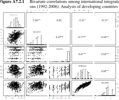
A7.2 Bivariate correlations
This chapter presents the bivariate correlations among independent variables. As explained in Chapter 7, the ratification of the UNFCCC was first analysed based on the developing-country sample. Therefore, Figures A7.2.1-A7.2.4 present the cor- relations for the developing-country sample from 1992-2006. In accordance with the analysis of the Kyoto Protocol ratification in Chapter 7, Figures A7.2.5-A7.2.8 present the bivariate correlations among independent variables for the pooled sam- ple from 1998-2006.
Figure A7.2.1 Bivariate correlations among international integration dimensi- ons (1992-2006): Analysis of developing countries
Notes: Analysis units = country-years.
Figure A7.2.2 Bivariate correlations among government ideology, veto player heterogeneity, and veto points (1992-2006): Analysis of develo- ping countries
Notes: Analysis units = country-years.
Figure A7.2.3 Bivariate correlations among political corruption dimensions (1992-2006): Analysis of developing countries
Notes: Analysis units = country-years.
Figure A7.2.4 Bivariate correlations among regime type, and democracy qual- ity measures (1992-2006): Analysis of developing countries
Notes: Analysis units = country-years.
Figure A7.2.5 Bivariate correlations among international integration indicators (1998-2006): Global comparative analysis
Notes: Analysis units = country-years.
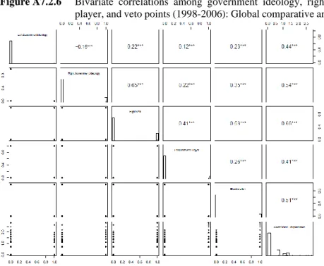
Figure A7.2.6 Bivariate correlations among government ideology, right veto player, and veto points (1998-2006): Global comparative analysis
Notes: Analysis units = country-years.
Figure A7.2.7 Bivariate correlations among political corruption dimensions (1998-2006): Global comparative analysis.
Notes: Analysis units = country-years.
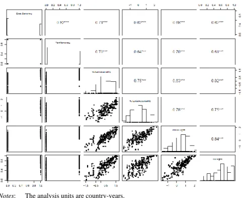
Notes: The analysis units are country-years.
A7.3 UNFCCC ratification
This chapter displays the results of the analysis of the additive effects of globalisa- tion and domestic political institutions on UNFCCC ratification. As described in Chapter 7, multiple models were estimated to reduce model complexity.
Figure A7.2.8 Bivariate correlations among regime type and democracy qualities in-
dicators (1998-2006): Global comparative analysis
Table A7.3.1 International integration and UNFCCC ratification (Global comparative analysis)
(1) (2) (3) (4) (5) (6)
Economic de- velopment
(ln)
-0.018 -0.032 -0.026 -0.022 0.005 -0.0358 (0.123) (0.121) (0.123) (0.125) (0.127) (0.132) Industry sec-
tor size (ln)
-0.386 -0.386 -0.400 -0.513 -0.412 -0.472 (0.354) (0.350) (0.353) (0.342) (0.366) (0.359) Fuel exports
(ln)
-0.065 -0.048 -0.064 -0.065 -0.008 0.040
(0.096) (0.095) (0.097) (0.096) (0.097) (0.099) ENGO
strength (ln)
0.458*** 0.448*** 0.477*** 0.480*** 0.358*** 0.428***
(0.130) (0.130) (0.130) (0.132) (0.134) (0.132) Population
density (ln)
-0.020 -0.017 -0.036 -0.053 -0.025 -0.019 (0.088) (0.086) (0.087) (0.085) (0.087) (0.086) Climate
change vul- nerability
-4.080*** -4.154*** -3.849*** -3.670*** -4.509*** -4.641***
(1.082) (1.072) (1.054) (1.048) (1.064) (1.069) Regional
commitment
3.630*** 3.677***
(0.666) (0.685) Annex I -0.631* -0.669* -0.683** -0.738** -0.876** -0.789**
(0.350) (0.350) (0.346) (0.348) (0.359) (0.347) Trade open-
ness (lg)
-1.181* -1.167* -0.737 -0.994 -0.919
(0.664) (0.664) (0.553) (0.678) (0.681)
Capital open- ness (ln)
0.161 0.168 0.0285 0.138 0.166
(0.133) (0.133) (0.109) (0.130) (0.129)
Policy diffu- sion
1.277** 1.299** 1.263**
(0.599) (0.601) (0.596)
IGO member- ships
0.016** 0.020*** 0.019*** 0.020*** 0.014**
(0.007) (0.006) (0.006) (0.006) (0.006) Network cen-
trality
0.253**
(0.121)
N 412 412 412 413 412 410
Notes: The table presents beta coefficients and standard errors in parentheses. * p < .1, **
p < .05, *** p < .01. Analysis units = country-years.
Table A7.3.2 Veto points and UNFCCC ratification (Global comparative ana- lysis)
(1) (2) (3) (4) (5) (6) (7) (8)
Economic devel- opment (ln)
-0.014 0.011 -0.003 -0.037 0.006 0.027 0.020 -0.011 (0.125) (0.123) (0.121) (0.124) (0.129) (0.127) (0.126) (0.127) Industry sector
size (ln)
-0.246 -0.332 -0.340 -0.288 -0.333 -0.382 -0.391 -0.348 (0.357) (0.353) (0.353) (0.358) (0.365) (0.364) (0.364) (0.366) Fuel exports (ln) -0.104 -0.100 -0.087 -0.074 -0.030 -0.0313 -0.027 -0.009 (0.100) (0.100) (0.098) (0.100) (0.100) (0.099) (0.098) (0.097) ENGO strength
(ln)
0.565*** 0.526*** 0.569*** 0.469*** 0.436*** 0.405*** 0.431*** 0.378***
(0.145) (0.137) (0.143) (0.133) (0.145) (0.140) (0.144) (0.136) Population den-
sity (ln)
-0.006 -0.013 -0.016 -0.010 -0.016 -0.017 -0.025 -0.016 (0.086) (0.087) (0.086) (0.087) (0.085) (0.086) (0.085) (0.086) Climate change
vulnerability
-4.153*** -4.167*** -4.197*** -4.011*** -4.581*** -4.594*** -4.615*** -4.467***
(1.104) (1.087) (1.090) (1.102) (1.088) (1.071) (1.076) (1.079) Regional commit-
ment
3.538*** 3.606*** 3.596*** 3.562***
(0.665) (0.665) (0.665) (0.665) Annex I -0.598 -0.512 -0.738** -0.521 -0.869** -0.795** -0.963*** -0.791**
(0.373) (0.356) (0.354) (0.357) (0.384) (0.364) (0.366) (0.366) Government frag-
mentation (ln)
-0.051 -0.342 -0.002 -0.249
(0.269) (0.220) (0.269) (0.215)
Bicameralism -0.504 -0.551* -0.385 -0.415
(0.367) (0.315) (0.365) (0.314)
Presidential veto player
-0.692 -0.728* -0.573 -0.598
(0.454) (0.423) (0.448) (0.412)
Trade openness (lg)
-1.157* -1.176* -1.156* -1.204* -0.935 -0.969 -0.921 -1.013 (0.662) (0.658) (0.669) (0.658) (0.677) (0.672) (0.684) (0.671) Capital openness
(ln)
0.108 0.139 0.161 0.106 0.100 0.121 0.133 0.101
(0.137) (0.134) (0.134) (0.137) (0.132) (0.130) (0.131) (0.132) Policy diffusion 1.487** 1.378** 1.450** 1.344**
(0.590) (0.596) (0.594) (0.595)
IGO memberships 0.017** 0.017*** 0.017** 0.016** 0.015** 0.015** 0.015** 0.014**
(0.007) (0.007) (0.007) (0.007) (0.007) (0.006) (0.007) (0.006)
N 406 411 407 407 406 411 407 407
Notes: The table presents beta coefficients and standard errors in parentheses. * p < .1, **
p < .05, *** p < .01. Analysis units = country-years.
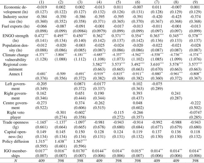
Table A7.3.3 Government ideology, right veto player, and UNFCCC ratifica- tion (Global comparative analysis)
(1) (2) (3) (4) (5) (6) (7) (8) (9)
Economic de- velopment (ln)
-0.019 0.002 0.002 -0.013 0.011 -0.007 0.011 -0.007 0.001 (0.127) (0.122) (0.127) (0.132) (0.126) (0.131) (0.128) (0.129) (0.129) Industry sector
size (ln)
-0.384 -0.350 -0.386 -0.395 -0.395 -0.391 -0.420 -0.425 -0.374 (0.360) (0.352) (0.358) (0.371) (0.365) (0.370) (0.367) (0.368) (0.368) Fuel exports (ln) -0.066 -0.087 -0.091 -0.001 -0.017 -0.013 -0.011 -0.001 -0.013
(0.098) (0.099) (0.0984) (0.0979) (0.099) (0.099) (0.097) (0.097) (0.099) ENGO strength
(ln)
0.472*** 0.495*** 0.450*** 0.362** 0.371*** 0.354** 0.363*** 0.345*** 0.378***
(0.141) (0.134) (0.140) (0.142) (0.137) (0.142) (0.136) (0.133) (0.137) Population den-
sity (ln)
-0.012 -0.020 -0.003 -0.025 -0.024 -0.020 -0.022 -0.021 -0.028 (0.088) (0.086) (0.085) (0.087) (0.086) (0.086) (0.087) (0.087) (0.087) Climate change
vulnerability
-4.371*** -3.804*** -4.181*** -4.685*** -4.357*** -4.562*** -4.558*** -4.736*** -4.374***
(1.128) (1.088) (1.112) (1.108) (1.073) (1.102) (1.085) (1.099) (1.076) Regional com-
mitment
3.582*** 3.573*** 3.492*** 3.610*** 3.578*** 3.577***
(0.663) (0.665) (0.663) (0.670) (0.663) (0.663) Annex I -0.681* -0.509 -0.691* -0.919** -0.815** -0.911** -0.880** -0.961*** -0.808**
(0.376) (0.356) (0.372) (0.382) (0.368) (0.382) (0.360) (0.372) (0.367) Left govern-
ment
-0.205 0.0871 -0.0177 0.102 -0.075
(0.349) (0.372) (0.337) (0.363) (0.289)
Right govern- ment
0.162 0.651 0.190 0.393 0.241
(0.346) (0.444) (0.344) (0.437) (0.287)
Centre govern- ment
-0.273 0.374 -0.262 0.048 -0.222
(0.522) (0.606) (0.515) (0.602) (0.502)
Right veto player
-0.301 -0.602* -0.115 -0.266 -0.0747
(0.274) (0.358) (0.272) (0.357) (0.285)
Trade openness (lg)
-1.165* -1.137* -1.097* -0.981 -0.943 -0.914 -0.992 -0.988 -0.943 (0.661) (0.664) (0.665) (0.678) (0.680) (0.684) (0.677) (0.679) (0.680) Capital open-
ness (ln)
0.149 0.145 0.150 0.128 0.124 0.119 0.137 0.136 0.118
(0.134) (0.134) (0.134) (0.131) (0.131) (0.132) (0.130) (0.130) (0.132) Policy diffusion 1.315** 1.438** 1.567***
(0.595) (0.601) (0.596) IGO member-
ships
0.017** 0.016** 0.0170** 0.0144** 0.014** 0.015** 0.014** 0.014** 0.014**
(0.007) (0.007) (0.007) (0.006) (0.006) (0.007) (0.006) (0.006) (0.006)
N 409 398 398 409 398 398 409 409 398
Notes: The table presents beta coefficients and standard errors in parentheses. * p < .1, **
p < .05, *** p < .01. Analysis units = country-years.
Table A7.3.4 Political corruption and UNFCCC ratification (Global compara- tive analysis)
(1) (2) (3) (4) (5) (6) (7) (8)
Economic de- velopment (ln)
-0.082 -0.117 -0.0463 -0.116 -0.081 -0.145 -0.031 -0.134 (0.133) (0.141) (0.126) (0.144) (0.135) (0.144) (0.130) (0.146) Industry sector
size (ln)
-0.255 -0.212 -0.334 -0.220 -0.242 -0.151 -0.347 -0.178 (0.373) (0.379) (0.358) (0.381) (0.384) (0.392) (0.370) (0.392) Fuel exports (ln) -0.048 -0.053 -0.053 -0.041 0.007 0.003 0.005 0.019
(0.097) (0.097) (0.097) (0.098) (0.098) (0.098) (0.098) (0.098) ENGO strength
(ln)
0.404*** 0.420*** 0.456*** 0.411*** 0.284** 0.300** 0.353*** 0.291**
(0.136) (0.131) (0.130) (0.134) (0.139) (0.134) (0.134) (0.136) Population den-
sity (ln)
-0.053 -0.051 -0.021 -0.040 -0.070 -0.069 -0.024 -0.052 (0.090) (0.090) (0.087) (0.088) (0.088) (0.088) (0.086) (0.086) Climate change
Vulnerability
-4.369*** -4.347*** -4.056*** -4.154*** -4.850*** -4.924*** -4.436*** -4.589***
(1.123) (1.106) (1.091) (1.090) (1.097) (1.085) (1.073) (1.067) Regional com-
mitment
3.707*** 3.789*** 3.612*** 3.722***
(0.664) (0.668) (0.664) (0.664) Annex I -0.814** -0.815** -0.697* -0.790** -1.168*** -1.224*** -0.974*** -1.164***
(0.384) (0.378) (0.362) (0.374) (0.402) (0.402) (0.376) (0.398) Executive cor-
ruption
-0.750 -1.060*
(0.596) (0.592)
Public sector corruption
-0.779 -1.200**
(0.544) (0.545)
Legislative cor- ruption
-0.088 -0.113
(0.104) (0.108)
Political corrup- tion
-0.840 -1.240*
(0.656) (0.662)
Trade openness (lg)
-1.122* -1.184* -1.255* -1.261* -0.847 -0.950 -1.055 -1.046 (0.668) (0.665) (0.669) (0.672) (0.689) (0.682) (0.680) (0.686) Capital open-
ness (ln)
0.146 0.151 0.151 0.141 0.093 0.107 0.114 0.087
(0.134) (0.133) (0.134) (0.134) (0.134) (0.131) (0.133) (0.133) Policy diffusion 1.209** 1.171** 1.218** 1.201**
(0.591) (0.591) (0.598) (0.592) IGO member-
ships
0.016** 0.017*** 0.016** 0.017** 0.014** 0.016** 0.014** 0.015**
(0.007) (0.007) (0.007) (0.007) (0.006) (0.006) (0.006) (0.006)
N 412 412 412 412 412 412 412 412
Notes: The table presents beta coefficients and standard errors in parentheses. * p < .1, **
p < .05, *** p < .01. Analysis units = country-years.