FAKULT ÄT F ÜR INFORMATIK DER TECHNISCHEN UNIVERSIT ÄT M ÜNCHEN

(1)

FAKULT ¨ AT F ¨ UR INFORMATIK

DER TECHNISCHEN UNIVERSIT ¨AT M ¨UNCHEN

Bachelorarbeit in Informatik

Probabilistic Cellular Automata

(2)

(3)

FAKULT ¨ AT F ¨ UR INFORMATIK

DER TECHNISCHEN UNIVERSIT ¨AT M ¨UNCHEN

Bachelorarbeit in Informatik

Probabilistic Cellular Automata Probabilistische Zellul¨are Automaten

Author: Carlos Camino

Supervisor: Univ.-Prof. Dr. Dr. h.c. Javier Esparza

(4)

(5)

I assure the single handed composition of this bachelor’s thesis only supported by declared resources.

(6)

(7)

Acknowledgments

I gratefully thank my advisor, Jan Kˇret´ınsk ´y, for his helpful comments and his infinite patience. I am also deeply grateful to Franziska Graßl, Pamela Flores and my brother Guillermo Camino for their unconditional help and support.

(8)

(9)

Abstract

Cellular Automata are mathematical, discrete models for dynamic systems. They consist of a large set of space-distributed objects that interact locally. It is known that the Major- ity Problem can only be solved by Cellular Automata with some limitations. This thesis presents Cellular Automata with a probabilistic extension and examins the performance of these Automata when solving this problem. These so-called probabilistic Cellular Au- tomata proved to perform better than the ordinary ones. However, another important criteria to be considered is the running time. This criteria is also examined.

Zusammenfassung

Zellul¨are Automaten sind mathematische, diskrete Modelle f ¨ur dynamische Systeme.

Diese bestehen aus einer großn Menge an räumlich verteilten Objekten die local wechsel- wirken. Es ist bekannt, dass das Mehrheitsproblem (Majority Problem) nur mit einigen Einschränkungen von zellulären Automaten gel öst werden kann. Diese Arbeit zeigt zel- luläre Automaten mit einer probabilistischen Erweiterung auf und untersucht die deren Leistung beim L ösen des Mehrheitsproblems. Diese sogenannte probabilistische zelluläre Automaten erwiesen sich als leistungsfähiger als gew öhnliche zelluläre Automaten. Den- noch ist die Laufzeit ein weiterer wichtiger Maßstab, der betrachtet werden muss. Dieser wird ebenfalls untersucht.

(10)

x

(11)

Outline of the Thesis

Part I: Introduction and Theory

CHAPTER1: PURPOSE OF THETHESIS

This chapter presents an overview of the thesis and its purpose.

CHAPTER2: INTRODUCTION TOCELLULARAUTOMATA

A short summary of the history of Cellular Automata and some examples of their applications are discussed here.

CHAPTER3: CHARACTERIZATION OFCELLULARAUTOMATA

In this chapter Cellular Automata are described in a more deeply and formal way including some variations of them.

CHAPTER4: MAJORITYPROBLEM

This chapter describes the Majority Problem for Cellular Automata. It also shows some of the most important published contributions to solve it.

Part II: Analysis and Conclusions

CHAPTER5: APPROACH

This chapter will give an overview about the implemented procedure of analyzing probabilistic Cellular Automata.

CHAPTER6: THETOOL

In order to analyze probabilistic Cellular Automata, a simulating tool is needed. The structure and functions of the implemented tool are presented here.

CHAPTER7: RESULTS

The most important results from the simulations are shown in this chapter.

CHAPTER8: CONCLUSIONS

The conclusions on this work will be discussed here.

(14)

(15)

Part I.

Introduction and Theory

(16)

(17)

1. Purpose of this Thesis

The task of programing massively parallel computing devices for solving problems has turned out to be difficult. One well known type of massively parallel computing systems are the so-called Cellular Automata. These are by definition very simple objects that can show behaviours of very high complexity. In order to analyze their computational power it is necessary to submit them to a well defined computational task. For Cellular Automata this task is par excellence theMajority Problem.

This thesis will aim to examine the computational power of Probabilistic Cellular Au- tomatausing the example of the Majority Problem. The search for a solution to it has concerned many theoretical computer scientists and mathematicians. Although it is known that it cannot be perfectly solved by ordinary Cellular Automata, there have been many attempts to get as close as possible to a perfect solution. This thesis will analyze a possible solution using Cellular Automata with a probabilistic extension and examine the circum- stances under which that solution is optimal. The nature of the topic dictates both the discussion of theoretical considerations and the use of a simulating tool in order to support them. This tool will mainly cover the following features:

1. Given the set of parameters that define a Probabilistic Cellular Automaton, a concrete problem specification and the maximum amount of time units, simulations of runs will be visualized. The tool will be able to recognize if the problem was correctly solved, if the computed solution was not correct or if the given maximum time units did not suffice to finish the computation. In addition it will output the amount of time steps needed for the run.

2. Providing the possibility to set any of the parameters as random values, the tool will be able to iteratively execute the same run a specified number of times providing the user with a statistic. This statistic will contain all the important information for the user to evaluate the performance of the Cellular Automaton defined by the given set of parameters. This information will regard the goodness and the average time units of the run.

3. In order to analyze the influence of a specific parameter on the performance of a Cellular Automaton, a last feature is required. This will allow the user to select one specific parameter and run many statistics, each of them with a different value for the chosen parameter, which will be increased gradually. The tool will finally display a graph showing the performance of the Cellular Automaton against that parameter.

Simulations ran using this tool will demonstrate the effects of probability and will give some evidence of what we can gain using Cellular Automata with a probabilistic extension.

(18)

1. Purpose of this Thesis

4

(19)

2. Introduction to Cellular Automata

ACellular Automaton(CA) is a mathematical, discrete model for dynamic systems. De- spite the simplicity of their construction CAs can exhibit very complex behaviors. This property makes CAs very popular among researchers from different areas including not only mathematicians and computer scientists, but also biologists, physicists, chemists, physicians, cryptographers, geographers, etc.

CAs are computational models based on some homogeneous components which can have one of a finite number of states. The state of each component changes through discrete time steps according to a defined transition rule and to the state of the components next to him. This is why, since their appearance in the 1950’s, CAs have mainly been used to model systems which can be described as a large set of space-distributed objects interacting locally, e.g. traffic flow, cells evolution, urban development,etc.

2.1. History of CA

CAs were introduced by John von Neumann in the late 1940’s while he was working on the problem of self-replicating systems [21]. Von Neumann had the notion of a machine constructing a replica of itself, but as he developed his design he realized that the costs of building a self-replicating robot were too high. Following a 1951 suggestion of Stanislaw Ulam (von Neumanns colleague at that time) he reduced his model to a more abstract, mathematical model. This reduction ended up 1953 in the first CA: one in which the components were ordered on a two-dimensional grid and each of them could have one of 29 different states and included an algorithmically implementation of his self-replicator. Von Neumann then proved the existence of a particular pattern which would make endless copies of itself within the given cellular universe. This design is known as the tessellation model and is called an universal constructor [20].

Later, in the 1960’s, CAs began to be studied as one type of dynamical systems and in 1970 a CA namedGame of Lifestarted to become widely known through the magazineSci- entific Americanby Martin Gardner [15]. This CA was invented by John Horton Conway and is one of the most known CAs today. Game of Life consists of a two-dimensional lattice in which each cell is colored black if the cell is “alive” and white if it is “dead”. The neighborhood is the so-called Moore-neighborhood: it consists of the 4 neighbors of von Neumann’s defined neighborhood (left, right, top and bottom side neighbors) and the 4 diagonal neighbors [22]. The transition rule for each cell is the following: 1) A dead cell becomes alive if it has exactly 3 living neighbors. 2) A living cell dies if it has less than 2 or more than 3 living neighbors (loneliness or overpopulation). 3) Otherwise a cell stays the same. In this game it is possible to build a pattern that acts like a finite state machine

(20)

2. Introduction to Cellular Automata

connected to two counters. The computational power of this machine is equivalent to the one of an universal Turing machine. This is why Game of Life is Turing complete, which means, that it is in theory as powerful as any computer with no memory limit and no time constraints [3].

Since 1983 Stephen Wolfram has done a lot of research in the field of CAs. He observed the evolution of one-dimensional CAs with 2 or 3 states and classified their behavior into 4 classes [25].

2.2. Applications

Despite their strong link to theoretical computer science CAs can be used in many other disciplines. In this section some concrete examples will be presented.

2.2.1. Mathematics

Wolfram [26] suggested in 1986 an efficient random sequence generator based on CA. For this he analyzed a one-dimensional CA in which each cell had one of only two states:

0 and 1. He discussed the use of rule 30 which shows, despite its simplicity, a highly complex evolution pattern which seems to be completely random (see figure 2.1). The time sequences created by this CA were analyzed by a variety of empirical, combinatorial, statistical, dynamical systems theory and computation theory methods.

Figure 2.1.: Chaotic behavior of rule 30 after 250 time steps. The rule was applied on an initial configuration consisting of only one black cell (state 1) surrounded by white cells (state 0). Source:

http://mathworld.wolfram.com/Rule30.html.

2.2.2. Biology

Green [16] has applied CAs in the field of ecology. He used CAs to represent tree loca- tions in simulations about forest dynamics. With these simulations he showed that forest dynamics are seriously affected by spatial patterns associated with fire, seed dispersal,

6

(21)

2.2. Applications

and the distribution of plants and resources. Ermentrout and Edelstein-Keshet [11] have applied CAs in other fields, such as developmental biology, neurobiology and population biology. They also described CAs that appear in models for fibroblast aggregation, branch- ing networks, trail following and neuronal maps.

2.2.3. Cryptography

Cryptographic systems are mathematical systems for encrypting or transforming information. In 1987 Guan [17] found that public-key cryptosystems could be based on CAs.

Having a string of binary bits (the plain text) which is supposed to be sent to a specific receptor, the major task of the cryptographic system is to cut the plain text into blocks of a specific length, saym, and then apply an invertible functionf :{0,1}^m→ {0,1}^mon each of them. This function should be easy to compute (for enciphering), its inverse should be hard to find (for deciphering by intruders), but with some key information the inverse im- age should be easy to compute. Considering the complex behavior of CAs, Guan proposed the use of aninvertibleCA to perform this conversion. He argues that the running time of all known algorithms for breaking the system grow exponentially withm.

2.2.4. Medicine

CA-models have been used to model many aspects of tumor growth and tumor-induced angiogenesis. Alarc ´on, Byrne and Maini [1] used a two-dimensional CA in which the cells could have one of 4 states: empty cell, cancer cell, normal cell and vessel. In order to consider blood flow (which most of the existing mathematical models at that time did not do) they developed their model in two steps. 1) First they determined the distribution of oxygen in a native vascular network. 2) Then they studied the dynamics of a colony of normal and cancerous cells placed in the resulting environment of step 1. Their most important result was that the heterogeneity of the oxygen distribution plays an important role in the restriction of cancerous colonies growth.

2.2.5. Geography

In 1993 Deadman, Brown and Gimblett [10] used a CA-based model to predict patterns of residential development. They used rules that changed according to the changing conditions and policies of the location and compared the obtained spatial patterns with mea- sured data. Their model presented strong structural significance, but also some predictive significance. As they write “It has the potential to be run into the future to predict the out- come of policy decisions”. A similar approach was carried out some years later by White, Engelen and Uljee [24]. They used a CA to represent the evolution of urban land-use patterns and got similar results: the predictions of their model were relatively accurate and suggested that CA-based models may be useful in a planning context.

(22)

2. Introduction to Cellular Automata

8

(23)

3. Characterization of Cellular Automata

There is no widely recognized formal and mathematical definition of CAs. Nevertheless it is important to have a formal description as a starting point. For this, a very general but formal characterization of CAs will be presented. This characterization will comprehend most of the CAs described in the literature. Hence, a more concrete definition of CAs will be presented and at the end of this chapter we will discuss some special type of CAs and some important properties of them.

3.1. General definition

Despite the fact that no established definition of CAs exists, a CA is a tuple(S,C, η, C₀, φ,) where:

• Sis a finite set ofstates,

• Cis a (potentially infinite) set ofcells,

• η:C → C^kis a neighbourhood function,k∈N,

• C₀:C →Sis aninitial configuration(we can also denoteConf =S^CandC₀∈Conf), and

• φ:S^k→Sis the so-calledtransition rule(also known as thelook-up tableor simply rule)

To describe the temporal behavior of the CA, a last function is needed. Let us call it thetransition functionΦ. This function is thenΦ : Conf → Conf defined byΦ(C)(c) = ϕ(C(c₁), . . . , C(c_k))where(c₁, . . . , c_k) =η(c).

This definition of CAs is very general and additionally too abstract for this purpose. For this reason it is appropriate to present an alternative, more concrete one.

3.2. Alternative definition

Both in the application areas for CAs presented in section 2.2 and in the CAs presented in the second part of this thesis, the arrangement of the cells within the configuration plays a significant role. For this reason it is required to make an alternative definition by changing the configuration from a multiset of unordered elements to a d-dimensional lattice. The other elements are defined almost analogously. In order to understand the idea of this new definition let us first introduce it ford= 1. Subsequently, the casesd= 2andd >2 will be sketched.

(24)

3. Characterization of Cellular Automata

3.2.1. One-dimensional lattice For the moment letdbe 1.

• Theconfigurationat timetis an infinite vector containing the ordered cells:

c_t= (. . . , c⁻¹_t , c⁰_t, c¹_t, . . .).

• For simplicity reasons let the set ofstatesbeS ={0,1, . . . , q−1}.

• Theneighborhoodof a cellcⁱ_tat timetis parameterized by aradiusrand is defined asη(cⁱ_t) = (c^i−r_t , . . . , cⁱ_t, . . . , c^i+r_t )∈S^2r+1. Each cell has then2r+ 1neighbors.

• Thetransition ruleis also parameterized byrbut its functionality stays the same. It maps the state values of all neighbors from one cell to its new state value:φ(η(cⁱ_t)) = cⁱ_t+1.

Thetransition function Φfor describing the temporal behavior of the CA has also the same functionality as described in section 3.1. The only difference is the formal definition of the mapping:Φ(c_t) = (. . . , φ(η(c⁻¹_t )), φ(η(c⁰_t)), φ(η(c¹_t)), . . .) =c_t+1. A one-dimensional (d = 1), two-state (q = 2), three-neighbor (r = 1) CA is called an elementary Cellular Automaton.

3.2.2. Two-dimensional lattice

Let nowdbe 2. Consider the cellsc^i,j_t to be ordered in respect of two indexesiandjon a two-dimensional lattice. The set of states and the look-up table remain the same, whereas the configuration, the neighborhood, and the transition function can be described using matrices instead of vectors. We obtain:

• Theconfigurationat timetas a matrix containing the ordered cells:

c_t=







. .. ... ... ... ...

· · · c^−1,−1_t c^−1,0_t c^−1,1_t · · ·

· · · c^0,−1_t c^0,0_t c^0,1_t · · ·

· · · c^1,−1_t c^1,0_t c^1,1_t · · · ... ... ... ... . ..







• The same set ofstates:S ={0,1, . . . , q−1}.

• The neighborhoodof a cellc^i,j_t at timetincluding all cells within the radiusrboth vertically and horizontally:

η(c^i,j_t ) =







cî−r,j−r_t · · · cî−r,j_t · · · cî−r,j+r_t ... . .. ... ... ... cî,j−r_t · · · cî,j_t · · · cî,j+r_t

... ... ... . .. ... cî+r,j−r_t · · · cî+r,j_t · · · cî+r,j+r_t







∈S(2r+1)×(2r+1)

10

(25)

3.3. Variations

Each cell has then(2r+ 1)²neighbors.

• The functionality of thetransition rulestays the same again:φ(η(cⁱ_t)) =cⁱ_t+1.

The functionality of the transition function Φalso stays unchanged. The difference is, again, the arrangement of the resulting elements:

Φ(c_t) =







. .. ... ... ... ...

· · · φ(η(c^−1,−1_t )) φ(η(c^−1,0_t )) φ(η(c^−1,1_t )) · · ·

· · · φ(η(c^0,−1_t )) φ(η(c^0,0_t )) φ(η(c^0,1_t )) · · ·

· · · φ(η(c^1,−1_t )) φ(η(c^1,0_t )) φ(η(c^1,1_t )) · · ·

... ... ... ... . ..







=c_t+1

3.2.3. d-dimensional lattice

For d ∈ N, d > 2 the cells cⁱ_t⁰^,i¹^,...,i^d−1 are ordered in respect to dindexes i0, i1, . . . , id−1

on a d-dimensional lattice and each cell has (2r + 1)^d neighbors. This case is not very interesting, since such CAs are rarely used (to best of the author’s knowledge there are no papers which are concerned with CAs with more than 2 dimensions). Furthermore, its definition would not contribute to the understanding of this thesis, but probably to the confusion of the reader.

3.3. Variations

The difference between the general and the alternative definition explained above is the design of the configuration. In the same way there is a possibility of making variations on the remaining components. This chapter shall depict some of these variations.

3.3.1. Boundary conditions

According to our definitions, the configuration of a CA consists of an infinite number of cells. However, for practical issues, it might be necessary to take some limitations into consideration. This is the case when using CAs in a modelling context as the memory of computers is finite. These considerations lead to the necessity of defining the boundaries of the now finite configuration. Some examples for this are:

Open boundaries We assume that cells with constant state values exist outside of the lattice. These cells are used to compute the new state of the border cells, but they do never change their state. We could, for example, define in the Game of Life some “dead open borders”. For this we set the state of all cells around the lattice as “dead”. This would represent a scenario in which it is impossible for a cell (or whatever a cell represents) to live outside of the lattice, e.g. an island.

(26)

Reflective boundaries The reflective borders consist of cells that “reflect” the state of the border cells. This case is similar to the open borders but with cells of varying state outside of the lattice. These cells change their state according to the actual state of the border cells as if the boundary was a mirror.

Periodic boundaries Another possibility is to “fold” the lattice so that two endings border to each other. For d = 1 this means a circular lattice. For d = 2 there are many possibilities. Some of them are depicted in figure 3.1.

(a) Sphere. (b) Real projective plane. (c) Klein bottle. (d) Torus.

Figure 3.1.: Fundamental polygons representing some possibilities of folding a two- dimensional lattice. The color of the arrows indicate which two endings should border to each other. The direction of the arrows indi- cates how both endings are to be oriented before folding them. Source:

http://en.wikipedia.org/wiki/Fundamental_polygon.

3.3.2. Cell arrangement

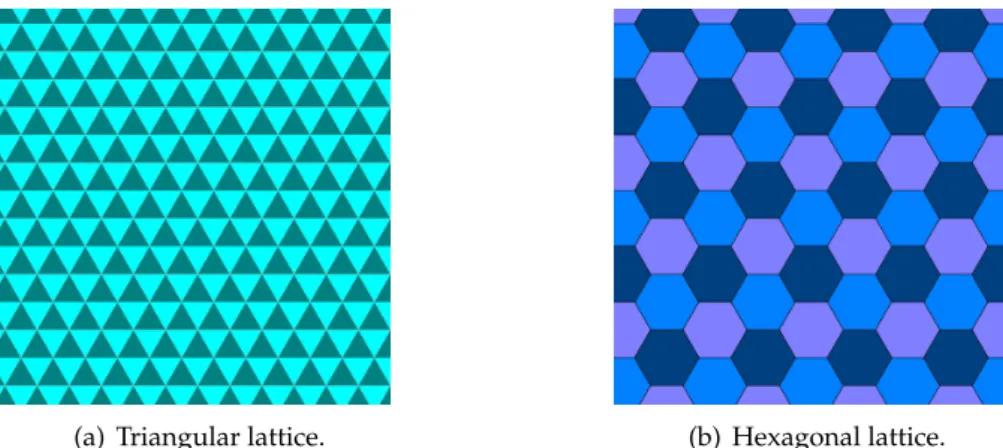
Concerning the arrangement of the cells, there are other possibilities than onlyd-dimensional lattices. For example, in a two-dimensional CA we assume that the cells are squares. We could change their form to triangles or hexagons and define their neighborhood according to the new arrangement (see figure 3.2).

12

(27)

3.3. Variations

(a) Triangular lattice. (b) Hexagonal lattice.

Figure 3.2.: Two possible CAs with two-dimensional lattices of non-squared cells. In the depicted cases the cells could have two (a) and three (b) different states. Source:

http://en.wikipedia.org/wiki/Hexagonal_lattice.

3.3.3. Neighborhood definition

Of course, independently from the border conditions and the cell arrangement, we can also change the definition of a cell’s neighborhood so that it is not well-defined by one parameterr. A good example to illustrate this is the difference between thevon Neumann neighborhood[23] and theMoore neighborhood[22] (see figure 3.3).

(a) The von Neumann neighborhood. (b) The Moore neighborhood.

Figure 3.3.: The von Neumann and the Moore neighborhood forr ∈ {0,1,2,3}. Sources:

see [23] and [22].

3.3.4. Transition rule determination

This variation is very important to understand this thesis. The CAs defined above consider one deterministic transition rule φ. This means that for each input the output is deter- minable. Another possibility to defineφis by using probabilistic elements. Aprobabilistic

(28)

Cellular Automaton(PCA) uses arandom variableX: Ω→ {0,1, . . . , m−1}and defines a probabilistic transition ruleφusing some deterministic transition rulesφ₀, φ₁, . . . , φm−1:

φ(η(cⁱ_t)) =











φ0(η(cⁱ_t)) ifX = 0, φ1(η(cⁱ_t)) ifX = 1,

...

φm−1(η(cⁱ_t)) ifX =m−1.

14

(29)

4. Majority Problem

TheMajority Problemis perhaps the most studied computational task for CAs. It consists of finding the best transition rule for a one-dimensional, two-state (S = {0,1}) CA that best performs majority voting. This means that the CA must recognize whether there are more 0’s than 1’s or more 1’s than 0’s in its initial configuration (IC) and within a given number of time units converge to a homogeneus configuration. This final homogeneus configuration must then consist of only 1’s if the number of 1’s in the IC was greater or vice versa.

The Majority Problem would be trivial for a computer with a central control unit. In contrast, for CAs this represents a real challenge, since they can only tranfer information at a finite speed relying only on local information, while the Majority Problem demands the recognition of a global property. For this reason this task is a good example of the phe- nomenon ofemergence in complex systems. This means, that its solution is an emergent global property of a system of locally interacting agents.

For a CA withr = 1(i.e. 3 neighbors) and perhapsr = 2(i.e. 5 neighbors) an exhaustive evaluation of all 2²^2r+1 rules would come into consideration. In these cases the task of finding the rule that performs best would be trivial. However, there is no scientific paper claiming the finding of a one- or two-radius rule that perfectly solves this problem. Hence, the most studied case nowadays is forr= 3(i.e. 7 neighbors). The purpose of this chapter is to present the Majority Problem and the most relevant approaches to solve it. The existence of a perfect solution is discussed in the last section.

4.1. Problem statement

The Majority Problem is a special case of theDensity Classification Problem, which can be defined as follows: Given an one-dimensional, two-state Cellular Automaton with initial configurationc0 consisting ofacells with state 1 and b cells with state 0, a ruleφand a density thresholdρ∈[0,1], the Density Classification Problem is considered to be:

• unspecified, if _a+b^a =ρ,

• solved, if∃t⁰.∀t.(t > t⁰ =⇒(_a+bâ < ρ∧c_t={0}â+b)∨(_a+bâ > ρ∧c_t={1}â+b)),

• unsolved, otherwise.

The Majority Problem corresponds to the Density Classification Problem forρ = ¹₂. The task is then to find a ruleφthat performs best. For this we define thequalityof a ruleφ as the fraction of all2^a+b ICs for whichφsolves the problem. However, since in most of

(30)

4. Majority Problem

the cases it is impossible to test all possible ICs we will define theperformanceof aφ(de- notedP_Nⁿ(φ)) as the fraction ofN randomly generated ICs of lengthnfor whichφsolves the problem and use it instead of the quality as an indicator of efficiency.

There are some conventions that have been indirectly established since the first attempt to solve this problem:

• To avoid the unspecified case _a+b^a =ρit is common to use odd numbers for the lattice sizen.

• It is also common the use of periodic boundaries (see 3.3.1).

• The rules are often encoded as a bit string by listing its output bits in lexicographic order of neighborhood configuration. This means that the string starts with the value ofφ((0, . . . ,0)) and ends with the value ofφ((1, . . . ,1)). The length of a such a bit string is2^2r+1.

4.2. Human-writen solutions

According to the definition and the quality measurement discussed above, there have been many propositions in the last 30 years for solving the Majority Problem. Some of them were designed “by hand” and some others by any heuristic methods. The first human- writen solution was created by G´acs, Kurdyumov and Levin in 1978 [14]. They created a rule (known as GKL ruleaccording to their names) while studying reliable computation under random noise. Their rule had a performance of about 81.6% withn= 149and N = 10⁶.

This rule is surprisingly efficient, although, there have been other hand-coded attempts to create better rules. In 1993 Davis [9] modified the GKL-rule and created a rule with 0.02% better performance. Two years later, Das [6] did the same and scored 0.378% better than Davis.

4.3. Evolved solutions

Mitchel has done a lot of research on the emergence of synchronous CA strategies during evolution. One of her most important research with regard to the Majority Problem is the one presented with Das and Crutchfield in [8]. They evolved rules using agenetic algo- rithm(GA) operating on fixed-length strings. Their GA starts with a random set of rules (calledchromosomes in the first generation) and evolved them to get better performances.

The evolution from one generation of rules into the next one is specified the following way:

1. A new set of random ICs is generated.

2. The performance of each rule is calculated

3. The population of rules is ranked in order of performance.

16

(31)

4.4. Overview

4. The best of them (the so called elite) are copied without modification to the next generation

5. The remaining rules for the next generation are formed by single-point crossovers between randomly chosen pairs of the elite with replacement.

6. Each of the resulting rules from the crossovers is then mutated a fixed number of times before it passes to the next generation.

They observed that in successful evolution experiments, the performance of the best rules increased according to what they calledepochs. Each epoch corresponds to a new, better solution strategy. They also observed that the final rules produced by this evolutional process showed in most of the runs unsophisticated strategies that consisted in expanding large blocks of adjacent 1’s or 0’s. Most of these rules had performances between 65% and 70%. The best result obtained using this method was 76.9%.

Mitchel and coworkers are still actively working on solving problems of collective be- haviour in CAs. In 1995 they adapted their work on the Majority Problem to theSynchro- nisation Problem, which led to better results: Their synchronisation rule φ_sync reached a performance of 100% [7].

Andreet al.were able to evolve rules usinggenetic programming(GP) with automatically defined functions [2]. They did not represent the chromosomes as boolean strings, but as functions{0,1}^2r+1 → {0,1}. Then they evolved them using the GP paradigm of representing them as tree structures and using the same operators as in the GA. In this case a crossover consisted of switching nodes between different chromosomes and a mutation consisted of replacing the information of a node by another. For each node they used functions{0,1} × {0,1} → {0,1}The results show the success of this method. Their evolved rule achieved an accuracy of 82.326% which was better than any known rule by that time.

Finally, Juill´e and Pollack presented a significant improvement for the Majority Problem by using acoevolutionary learning(CL) method [18]. CL involves the embedding of adaptive learning agents in a fitness environment that dynamically responds to their progress. With this method they evolved a rule with a performance of about 86.3%. This is the best result known to date.

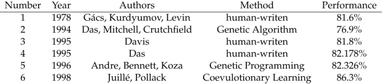
4.4. Overview

A summary of all the rules for solving the Majority Problem discussed here is presented in table 4.1. Their explicit string representation (from bit 0 to bit 127) are presented in table 4.2. All experiments were carried out on a lattice withn= 149cells.

4.5. Perfect Solution

The probably most interesting question regarding the Majority Problem is how effective a rule can possibly be. Despite the fact that this is still an open question, there have been

(32)

4. Majority Problem

Number Year Authors Method Performance

1 1978 G´acs, Kurdyumov, Levin human-writen 81.6%

2 1994 Das, Mitchell, Crutchfield Genetic Algorithm 76.9%

3 1995 Davis human-writen 81.8%

4 1995 Das human-writen 82.178%

5 1996 Andre, Bennett, Koza Genetic Programming 82.326%

6 1998 Juill´e, Pollack Coevulotionary Learning 86.3%

Table 4.1.: Summary of the most important solutions

Number Rule

1 00000000 01011111 00000000 01011111 00000000 01011111 00000000 01011111 00000000 01011111 11111111 01011111 00000000 01011111 11111111 01011111

2 N/A

3 00000000 00101111 00000011 01011111 00000000 00011111 11001111 00011111 00000000 00101111 11111100 01011111 00000000 00011111 11111111 00011111 4 00000111 00000000 00000111 11111111 00001111 00000000 00001111 11111111 00001111 00000000 00000111 11111111 00001111 00110001 00001111 11111111 5 00000101 00000000 01010101 00000101 00000101 00000000 01010101 00000101 01010101 11111111 01010101 11111111 01010101 11111111 01010101 11111111 6 00010100 01011111 01000000 00000000 00010111 11111100 00000010 00010111 00010100 01011111 00000011 00001111 00010111 11111111 11111111 11010111 Table 4.2.: Bit string representation of the most important solutions

some attempts to find at least a partial answer to it. In 1995 Land and Belew proved that there exists no two-state CA with finite radius that perfectly solves the Density Classifica- tion Problem [19]. Assuming that such a CA exists, they considered a sequence of initial configurations in which the Majority Problem cannot always be solved. They argue that, since the system is deterministic, every cell surrounded only by cells with the same state must turn to the same state as the cells surrounding it. The same way, any rule that performs majority voting perfectly can never make the density pass over theρthreshold. They show that in the case of a single standing cell, any assumed perfect rule would do one of two unpermitted things: 1) if the fraction of cells with the same state as the isolated cell is greater thanρthen the rule would cancel the state of that cell out and cause the density to cross theρthreshold, or 2) if the fraction of cells with the same state as the isolated cell is less thanρthen the rule would convert the state of some cells to the state of the isolated cell causing the ratio to become greater thanρ.

Their difficulties in evolving a better solution than the one presented by Das, Mitchell and Crutchfield in [8] led them to question if such a CA exists. However, the same way variations of CAs exist, there have also been made some changes on the Majority Problem in order to reach solutions with 100% quality.

18

(33)

4.5. Perfect Solution

One year after Land and Belew proved the non-existence of a perfect rule, Capcarre, Sip- per and Tomassini published a method to solve the Majority Problem by simply changing the output specification [4]. If _a+bâ > ¹₂ the final configuration should consist of one or more blocks of at least two consecutive 1’s mixed by an alternation of 0’s and 1’s, in the case _a+bâ < ¹₂ it should consist of one or more blocks of at least two consecutive 0’s mixed by an alternation of 0’s and 1’s, and if _a+bâ = ¹₂ it should consist only of an alternation of 0’s and 1’s (see figure 4.1). For this they used an elementary Cellular Automaton (see 3.2.1) with the following rule:

φ₁₈₄(η(cⁱ_t)) =

(cⁱ⁻¹_t , ifcⁱ_t= 0, cⁱ⁺¹_t , ifcⁱ_t= 1,

This rule is known asrule 184because of the interpretation of its string representation as a decimal number. In their work, Two-state, r=1 Cellular Automaton that Classifies Density, they prove the property of rule 184 to solve this modified version of the Majority Problem by using 4 lemmas. These are important to understand the main properties of rule 184, which is fundamental for this thesis.

Figure 4.1.: Example of the use of rule 184 on four initial configurations. White pixels represent cells with state 0, black pixels represent cells with state 1. The first 200 time steps of each simulation are presented. All four configurations have lattice sizen= 149. The initial configurations of (a), (b) and (c) were randomly generated, the one of (d) consists of 75 cells with state 1 and 74 with state 0.

Source: see [4]

Lemma 1. Density is maintained through time. Let D(ct) denote the density of the configuration at timet. This is the fraction ofncells that have state 1. This lemma states that∀t∈N. D(c₀) =D(c_t).

Lemma 2. Coexististing blocks annihilate each other if the 0’s are left from the 1’s. In case there exists a fragment of the configuration of the form: . . . , x,0, . . . ,0,1, . . . ,1, y, . . . with a block ofα0’s, a block ofβ 1’s andx, y ∈ {0,1}afterv=min{α, β} −1transitions the number of 0’s and the number of 1’s betweenxandywill be reduced byvrespectively.

(34)

4. Majority Problem

Lemma 3. Blocks of 0’s move from left to right. Blocks of 1’s from right to left. Mathe- matically this means:

(cⁱ_t, . . . , cî+α_t ) = (0, . . . ,0) =⇒(cⁱ⁻¹_t−1, . . . , cî−1+α_t−1 ) = (0, . . . ,0), (cⁱ_t, . . . , cî+α_t ) = (1, . . . ,1) =⇒(cⁱ⁺¹_t−1, . . . , cî+1+α_t−1 ) = (1, . . . ,1).

Lemma 4. There are no two blocks that coexist after timedⁿ₂e. This lemma follows di- rectly from lemma 2 and lemma 3 and from the periodic boundaries of the lattice. By combining it with lemma 1 the property of rule 184 to solve this problem can easily be proved.

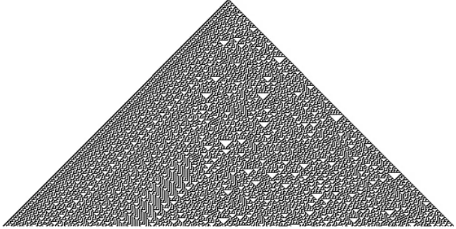
Another possibility to solve the Majority Problem is the one presented by Sipper, Cap- carrere and Ronald in 1998 [5]. Their approach also consists of changing the output specification, this time turning the periodic boundaries to open boundaries (the left cell is fixed at state 0 and the right one is fixed at state 1) and using again rule 184. The resulting configuration corresponds to the IC with sorted cells: 0’s to the left and 1’s to the right. An example of a run using this method is depicted in figure 4.2.

Figure 4.2.: Space-time diagram showing one solution to the Majority Problem’s version presented by Sipper, Capcarrere and Ronald in [5]. The lattice has sizen= 149.

The state of the cell at position ⁿ₂ is 1 (black), thusD(c0)> ¹₂.

In 1997, Fuk´s proposed the use of two elementary Cellular Automata to solve this problem [12]. He described the process as an assembly line consisting of two machines working one after the other. These machines represented two elementary CA, one of them using rule 184 and the other one usingrule 232. This rule can be defined as:

φ232(η(cⁱ_t)) =

(0, ifcⁱ⁻¹_t +cⁱ_t+cⁱ⁺¹_t ∈ {0,1}, 1, ifcⁱ⁻¹_t +cⁱ_t+cⁱ⁺¹_t ∈ {2,3}.

If there are more 1’s than 0’s in a cell’s neighborhood, this rule turns the state of that cell into 1. If there are more 0’s than 1’s, this rule turns the cell is set to state 1. This is why it is also known as themajority rule. This way, the first CA would useφ₁₈₄ to “stir” the cells to get the final configuration as described by Capcarre, Sipper and Tomassini in [4]. The second CA would useφ232to expand the remaining block of consecutive 0’s or 1’s until it

20

(35)

4.5. Perfect Solution

reaches the length ofn.

Fuk´s has also suggested the use of elementary diffusive probabilistic Cellular Au- tomata to solve this problem in a “non-deterministic sense” [13]. The transition rule of his diffusive PCA maps a cell’s state to 1 (or 0) with a probability proportional to the number of 1’s (or of 0’s) in its neighborhood. This means that his version of a PCA does not use the same random variableXat each application of the transition function. In fact, at each application ofφ, it uses a different random variable depending on the current states of the cell’s neighborhood.

(36)

4. Majority Problem

22

(37)

Part II.

Analysis and Conclusions

(38)

(39)

5. Approach

The goal of this thesis is to analyze the computational power of PCAs using the example of the Majority Problem. The use of rule 184 to “stir” the cells together with rule 232, as described by Fuk´s, suggests that the combination of them might lead to good results. For this reason this thesis will mainly discuss this combination. While Fuk´s used either more than one elementary CA [12] or more than one random variable in a PCA [13] to solve this task, we will focus on using one single elementary PCA that uses only one random variable. Note that the neighborhood of an elementary PCA consists of only 3 neighbors (r = 1), in opposition to the solutions presented in chapter 4 where CAs with 7 neighbors (r = 3) were used. We will show that with the probabilistic extension better results can be expected despite the small neighborhood.

Our PCA is (as described in 3.3.4) a CA that uses a random variableX : Ω → {0,1}to define its transition ruleφas follows:

φ(η(cⁱ_t)) =

(φ₁₈₄(η(cⁱ_t)) ifX= 0, φ232(η(cⁱ_t)) ifX= 1.

Letpbe the probability ofXbeing 1 and1−pthe probability ofXbeing 0, mathematically this is written: P r[X = 1] =pandP r[X = 0] = 1−p. Having defined this probabilistic rule we would be able to start drawing conclusions, e.g. it is not difficult to see that the bigger the probability ofXto be 0, the better will be the performance of the rule (forp >0).

For this reason we will not only construct a PCA which performs best and run some simulations of it to get an approximation of its quality. Additionally the influence that some parameters might have on the performance of the PCA will be analyzed.

In this case it is not only important to consider the performance as the fraction of all randomly generated ICs which were correctly solved, but also to consider the time units needed to solve the problem. For this reason it is appropriate to define theaverage run- ning timeof a ruleφ(denotedT_Nⁿ(φ)) as the average of the time units needed inN runs on randomly generated ICs of lengthn. Of course the average running time is a statistical approximation of theexpected running time, which is too complex to calculate in this case. As in the works presented in chapters 4.2 and 4.3 we will rely on the law of large numbersto be able to substitute probability measures (e.g.quality, expected running time) by statistical ones (e.g.performance, average running time). Using these notations we are able to argue, taking the example presented above, that choosingp → 0is a bad strategy because we would indeed expectP_Nⁿ(φ)→1, butT_Nⁿ(φ)→ ∞which is suboptimal.

To perform this task a tool is needed in order to simulate different runs from different PCAs and compare them. This tool should allow the user to construct a PCA by typing

(40)

5. Approach

in the values of all parameters that define it (e.g. lattice size, density, rules, probability distribution, etc.) and plot one or many runs of it. These plots may vary depending on their purpose. It can be either

• aspace-time diagramdisplaying the evolution of one single run,

• abar chartshowing the performance and the average running time of a PCA afterN independent runs, or

• line chartsplotting the performance and the average running time of a PCA against one chosen parameter which is gradualy increased through its range.

This tool will then be used to generate and visualize the data that is necessary in order to examine and draw conclusions about a PCA’s behavior.

26

(41)

6. Tool

The task of the implemented tool is, as mentioned in chapter 5, to simulate single runs of a constructed PCA. The aim of this chapter is to present this tool. For this it will describe its components and explain their implementation in a very brief manner. This chapter is subdivided in 2 sections: The first one will discuss all parameters used to describe a simulation run and how they are organized. In this case, a simulation consists not only of a PCA, but also of a problem to be solved. Although this work will be exclusively concerned with the Majority Problem, other problems were also implemented for possible further in- vestigations beyond density classification. Section 2 will explain all three functionalities of the tool in a more detailed way than it was done in chapters 1 and 5.

The tool was developed within about 8 weeks and was programmed in Java using the NetBeans IDE.

6.1. Structure

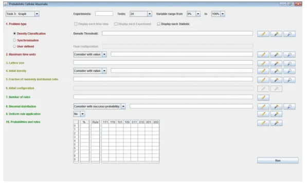
As aforementioned, a simulation can be characterized by a set of parameters. This set can be taken out of figure 6.1. Their names are listed at the left side of the window. In order to bring some structure into the program, the parameters were classified into three groups:

theProblem, theConfigurationand theRule. According to figure 6.1, items 1 and 2 belong to the Problem, items 3 to 6 to the Configuration, and the last 4 items to the Rule. Each group was implemented as an own java-class.

6.1.1. Problem

This is the first component. The Problem class defines which type of problem is to be solved. It includes the maximum amount of time units allowed to solve the problem and a problem-specific parameter (if required). For this class 3 different main instances exist:

the well-knownDensity Classification Problem, theSynchronisation Problem(as presented in [7]) and auser defined problemwhich allows the user to define its own final-configuration.

This class includes the implementation of a method that, depending on the problem type, the actual time unit and the actual configuration of the lattice recognize if the problem has been solved (correctly or incorrectly), if the maximum amount of time units has been reached, or if the next configuration has to be computed. The parameters of this class are the following:

Problem type Its value is an integer of {0,1,2}. Depending on this value, one of the three instances mentioned above is created. This parameter is important when checking the status of the run after each lattice update.

(42)

6. Tool

Figure 6.1.: Main window of the tool. The color used to write the name of each parameter depends on the component it belongs to. Red: Problem, yellow: Configuration and green: Rule.

Density threshold This parameter is optional, since it only requires a concrete value if the problem type is set for the Density Classification Problem. It represents the value of ρ∈[0,1]as described in chapter 4.1. If set to¹₂ the problem will correspond to the Majority Problem.

Final configuration The final configuration is represented as an array containing only 0’s and 1’s. It represents the configuration that is to be reached in order to solve a user defined problem. Of course, this parameter is also optional and requires a concrete value only in case of the user defined problem.

Maximum time units Since PCAs are non-deterministic automata, it is difficult to recognize for a specific configuration if the problem can still be solved or not. In case of a normal CA the program could stop as soon as it reaches a specific configuration that it had before. For this reason it is suitable to include an upper bound for the time units. In case the problem is not solved within this number of time steps, the run is considered not terminated. The value of this parameter is of{1, . . . ,1000}. For special cases two additional values are also allowed: 10000 and∞.

6.1.2. Configuration

The second important component is the Configuration class. This class represents the actual configuration of all cells in the lattice. After each time unit the Configuration-object is updated by adjusting all its parameters to the new lattice. In case that the tool has to

28

(43)

6.1. Structure

output not only the result, but the whole evolution of the lattice through the time, a copy of the relevant parameters are stored in a list. Otherwise only the initial and the actual configuration are stored in order to determine if the problem has been solved or not. This class has an implemented method that applies a rule (determined by a simulated random variable) to all cells. It also includes the following parameters:

Lattice size In order to avoid too high latencies the value of the lattice size n will be bounded by 200. This means thatn∈ {3, ...,200}.

Initial density This parameter representsD(c₀)∈[0,1]as described in chapter 4.5, Lemma 1) and is also optional. It can be used to test the performance of a rule combination on an IC with a determined density. If not set, the lattice will either be completely random, which means that the initial density will be binomial distributed centered at ⁿ₂, or it can be manually set by the user. If set to a concrete number, the program will set the first bn·(1−D(c0)) +¹₂c=bcells to 0 and the lastbn·D(c0) + ¹₂c=ato 1.

Fraction of randomly distributed cells This parameter is only considerediff the Initial density has also been considered. The value of this parameter determines the fraction of randomly chosen cells to be stirred with the rest of the cells. If its value is 0 the cells will be perfectly ordered: first b 0’s followed bya1’s. If its value is 1 all a+b cells will be randomly positioned in the lattice. All values within the range[0,1]are accepted.

Initial configuration This is the most important parameter for this class. It contains the values of all cells arranged in an array of integers.

6.1.3. Rule

The last important component is the Rule class. It defines the probabilistic rule that is to be applied on the configuration at each time step. As the two classes described above, an object of this class also consists of a set of parameters. These are:

Number of rules As used in chapter 3.3.4, the number of rules corresponds to the value ofm. For user-friendliness and because it is more than enough for our purpose, this parameter will be bounded by 10.

Success probability This is another optional parameter. It represents (as it name reveals) the parameterp∈[0,1]of a binomial distributed random variableX ∼Bin(n, p)in which n+ 1is the number of deterministic rules involved. With this parameter, it is possible to define the probabilities of all rules by changing only one value. This can be very useful when using only 2 rules. In that case pwould represent the probability of choosing the first rule (e.g, rule 184) and1−pthe probability of choosing the second one (e.g, rule 232).

Uniform rule application The value of this parameter is boolean: Iftrue, the rule to be applied will be chosen once for the whole lattice at each time step. Iffalse, the rule to be applied will be chosen for each cell independently.

(44)

6. Tool

Rules and probabilities These parameters include the concrete values of themrules that constitute the probabilistic rule used by the PCA and their concrete probabilities. These can either be set manually by the user, or depend on the succes probability.

6.2. Functions

As already mentioned, there are three main tasks the tool should perform. In chapter 1 a specification of them was presented. Furthermore, chapter 5 outlined their respective outputs in a very brief manner. This section will provide a more concrete and in-deep description of these three features which are each represented in the program as a class.

6.2.1. Experiment

AnExperiment simulates a run on a single PCA. An object of this class consists mainly of the three components aforementioned: a Problem, a Configuration and a Rule. At first, the values of their parameters are not initialized. This means that some of them might not have been set yet, e.g. the initial configuration is empty, because its content depends on the value of the initial density and the fraction of randomly distributed cells. Each of these components has an implementetinitialize()-method which correctly sets all values that depend on other ones.

The most important method in this class is therun()-method. Whenrun()is invoked, first all three components are initialized and a counter of time units is set to zero. Then the rule is iteratively applied to the configuration and the counter is increased by one. After each round, the status of the problem is checked by the Problem-object. This process is repeated until the problem is solved, or the maximum number of time units is reached.

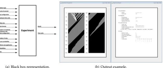
The evolution of the configuration during this process is stored in a list. When the run is finished and the result is known, the evolution of the configuration is taken from the list and drawn in a space-time diagram. This diagram is accompanied by a written report containing the input (i.e. the inserted values for all parameters) and output (i.e. the status

∈ {correctly solved,incorrectly solved,not terminated}and the number of time units needed) of the run.

Figure 6.2 presents an Experiment run as a black box and an example of an Experiment output. For analytical reasons a detailed output of the run is written in the console. This extra output includes the value of each cell, the value of the density, and the deterministic rule applied at each time unit to each cell.

30

(45)

6.2. Functions

(a) Black box representation. (b) Output example.

Figure 6.2.: Black box representation and output example of an Experiment run. (a) Input arrows are grouped by classes. Dashed arrows represent optional input parameters. (b) Left: The evolution of the PCA as a time-space diagram. White pixels represent cells with state 0, black pixels represent cells with state 1. Right: Writ- ten Report containing all important information about the input and output.

In case a random parameter is desired, a button for randomly generating values was implemented for almost each parameter. This button is identified with an icon of a pencil, see figure 6.1. When pressed, the program fills out the corresponding text field with a random value from a uniform distribution over all allowed values.

6.2.2. Statistic

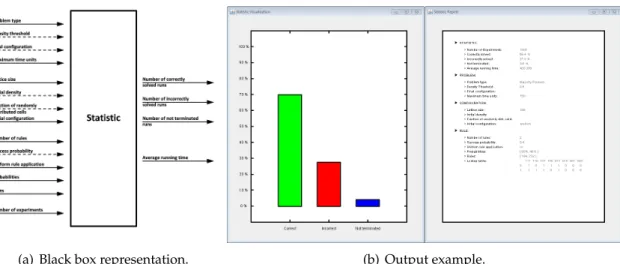
An object of theStatisticclass represents the repetition of many independent instances of the same run. Since PCA are non-deterministic, such a statistic makes always sense, even if no parameter has a random value. A Statistic-object consists of only two components: an Experiment object and an integer representing the number of Experiments to be ran,i.e.N.

The most important method in this class is also the run()-method. When invoked, a copy of the Experiment-object is created using the overwrittenclone()-method. The components of this copy are then initialized as described above, ran, and both results (status and time) are stored. This is repeated with a total ofN copies of the object. At the end, the accumulated results for the status are drawn in a bar-chart and their concrete values are presented together with the average running time and the input data in a written report. Figure 6.3 displays a black box representing the run of a Statistic and an example of a Statistic output.

(46)

6. Tool

Figure 6.3.: Black box representation and output example of an Statistic run. (a) Input arrows are grouped by classes. Dashed arrows represent optional input parameters. (b) Left: The amount of Experiments that were correctly solved (green), incorrectly solve (red) and did not terminate (blue) as a bar-chart. Right: Writ- ten Report containing all important information about the input and output.

When creating a Statistic, a second button for most of the parameters will be set enabled.

This button is identified with an icon of a magic wand (see figure 6.1) and allows to chose the value “random” for that parameter. This, in contrast to the first button, does not create a random value at that moment that remains constant through the run. In fact, the parameter gets a concrete, random value only when it is initialized. Since theinitialize()- method is only invoked on copies of the original Experiment-object, this allows each copy of the Experiment to have a different value from the others. This option is very useful when running simulations on random lattices.

6.2.3. Graph

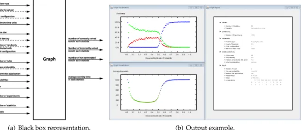
AGraph object represents the repetition of many independent, slightly different Statis- tics. Its components are a Statistic object and two integers: one representing the number of Statistic to be ran, sayM, and another one representing one of 6 parameters. I will refer to this parameter as thevariable. The variable can be chosen by pressing on the button identified with a magnifier icon (see figure 6.1). Since for the output, the variable is taken as the abscissa, only parameters with numerical values can be chosen to be the variable.

The run()-method from a Graph object works almost the same way as the run()- method from a Statistic object: It creates M copies of the Statistic object, runs them independently, and stores the results. The only difference is that the copied objects are not equal. The value of the variable is systematically increased during the copying process.

Each of the Statistics can be represented as two pairs: the first component of both pairs is the value of the variable, the second component is the accumulated status results for one pair, and the average running time for the other. This way the performanceP and average

32

(47)

6.2. Functions

running timeT can easilly be plotted against the chosen variable. The output consists of both plots and a written report. A black box representation of a Graph run and an example of Graph out are depicted in figure 6.4. In order to be able to manipulate the graphs, the arrays containing the coordinates of all pairs are also written in the console.

Figure 6.4.: Black box representation and output example of a Graph run. (a) Input arrows are grouped by classes. Dashed arrows represent optional input parameters. (b) Top left: TheGoodness-function. Ordinate: Fraction of correctly solved (green dots), incorrectly solved (red dots), and not terminated (blue dots) Ex- periments. The green dots representP. Abscissa: the variable. Bottom left:

T as a function. Each dot represents one Statistic. The three coordinates of each dot’s color (represented in the RGB color model) are proportional to the fraction of all three status. This is useful to recognize the estimate value ofP observing only theT-function. Right: Written Report containing all important information about the input and output.

(48)

6. Tool

34

(49)

7. Results

As mentioned in chapter 5, we will explore the computational power of PCAs on the ba- sis of the Majority Problem simulating them with the tool described in chapter 6. These PCAs will consist of only three neighbors (r = 1) and only one random variableXwhich determines the probability of using one of two rules:φ184orφ232at each time step. This chapter will present the most significant results obtained. In chapter 5 was mentioned that it is important to analyze not only the performanceP of the probabilistic ruleφbut also its average running timeT. The first section of this chapter will present an example run which depicts the reason for the importance of such an analysis. Moreover, it will explain the importance of the probability distribution betweenφ184 andφ232. In sections 2 and 3 a concrete analysis of the running time depending on this probability distribution will be carried out.

7.1. The importance of time analysis

In chapter 5 was also mentioned that a correlation between the probability of using rule 184 and the performance of the probabilistic rule exists. This correlation can be seen in figure 7.1. The green dots in the left graph represent the performance of the probabilistic ruleP(φ)as a function of the probability of using rule 232. In order to avoid the distortion of the green curve caused by the case of not terminated runs (blue dots), the maximum time units were set to infinity. The graph on the right represents the running time of the probabilistic ruleT(φ)as a function of the same probability.

Figure 7.1.: Output of a Graph run with the success probability as the variable with range [0.01,0.49]. Left: fraction of correctly solved, incorrectly solved and not terminated Experiments. Right: The average running time. For the computation of each dot 5000 Experiments were carried out. The lattice size was 149 and the configuration was randomly generated after each Experiment.