Women’s Empowerment and Socio-Economic Outcomes

(1)

Policy Research Working Paper 6841

Women’s Empowerment and Socio-Economic Outcomes

Impacts of the Andhra Pradesh Rural Poverty Reduction Program

G. Prennushi A. Gupta

The World Bank South Asia Region

Sustainable Development Department April 2014

WPS6841

Public Disclosure AuthorizedPublic Disclosure AuthorizedPublic Disclosure AuthorizedPublic Disclosure Authorized

(2)

Produced by the Research Support Team

Abstract

The Policy Research Working Paper Series disseminates the findings of work in progress to encourage the exchange of ideas about development issues. An objective of the series is to get the findings out quickly, even if the presentations are less than fully polished. The papers carry the names of the authors and should be cited accordingly. The findings, interpretations, and conclusions expressed in this paper are entirely those of the authors. They do not necessarily represent the views of the International Bank for Reconstruction and Development/World Bank and its affiliated organizations, or those of the Executive Directors of the World Bank or the governments they represent.

Policy Research Working Paper 6841

The paper explores whether one of the largest programs in the world for women’s empowerment and rural livelihoods, the Indira Kranti Patham in Andhra Pradesh, India, has had an impact on the economic and social wellbeing of households that participate in the program.

The analysis usespanel data for 4,250 households from two rounds of a survey conducted in 2004 and 2008 in five districts. Propensity score matching was used to construct control groups and outcomes are compared with differences-in-differences. There are two major impacts. First, the Indira Kranti Patham program increased participants’ access to loans, which allowed them to accumulate some assets (livestock and durables for the poorest and nonfarm assets for the poor), invest in education, and increase total expenditures (for the poorest and poor). Women who participated in the program had more freedom to go places and were less afraid to disagree with their husbands; the women

This paper is a product of the Sustainable Development Department, South Asia Region. It is part of a larger effort by the World Bank to provide open access to its research and make a contribution to development policy discussions around the world. Policy Research Working Papers are also posted on the Web at http://econ.worldbank.org. The authors may be contacted at gprennushi@worldbank.org and agupta20@worldbank.org.

participated more in village meetings and their children were slightly more likely to attend school. Consistent with the emphasis of the program on the poor, the impacts were stronger across the board for the poorest and poor participants and were more pronounced for long-term Scheduled Tribe participants. No significant differences are found between participants and nonparticipants in some maternal and child health indicators. Second, program participants were significantly more likely to benefit from various targeted government programs, most important the National Rural Employment Guarantee Scheme, but also midday meals in schools, hostels, and housing programs. This was an important way in which the program contributed to the improved wellbeing of program participants.

The effects captured by the analysis accrue to program

participants over and above those that may accrue to all

households in program villages.

(3)

Women's Empowerment and Socio-Economic Outcomes Impacts of the Andhra Pradesh Rural Poverty Reduction Program

G. Prennushi and A. Gupta Revised, March 2014

JEL Codes: D13; I24; J16; O15; O17

Keywords: Women's empowerment; rural community-level interventions; impact evaluation; India; Andhra Pradesh.

Sector: ARD, POV

_______________________________________

Prennushi: World Bank, 1818 H Street NW, Washington DC 20433 (e-mail: gprennushi@worldbank.org, gioprennushi@gmail.com). Gupta: World Bank, 1818 H Street NW, Washington DC 20433 (e-mail:

agupta20@worldbank.org). We are grateful to Vijayendra Rao, Parmesh Shah, and Shobha Shetty for guidance.

We thank B. Rajsekhar, A. Murali, N. Reddy (SERP), S. Galab (CESS) and other colleagues at SERP and CESS for very valuable inputs on the program and the data. We would also like to thank Luis Alberto Andres, Ritam

Chaurey, Pedro Carneiro, Klaus Deininger, Jon Jellema, Priti Kumar, Yanyan Liu, Sitaram Machiraju, Jeeva Perumalpillai-Essex, and Forhad Shilpi for their comments. Financial support from DFID, SAFANSI, and SERP is gratefully acknowledged.

(4)

1. Introduction

Programs that seek to improve the lives of the rural poor through their mobilization into groups, often focused on women, have expanded considerably in recent years. Many of these programs started with social mobilization and microfinance activities and expanded over time to include interventions to build up productive capacity and improve access to human development and other public services. While these community-driven development and rural livelihoods

interventions have spread, rigorous evidence on their impact is limited, particularly on economic indicators.

Available studies include an evaluation of the Kecamatan Development Program in Indonesia (Voss, 2008), which found no impact on average household consumption, but gains for the poorest and the richest 20 percent of the households, with per capita consumption levels increasing by about 5 percent as a result of the program. Mansuri and Rao (2012) reviewed several studies and concluded that, in general, the better-off participate more and benefit more and that impacts on poverty are elusive. Recently, an evaluation of the Poverty Alleviation Fund in Nepal (Acharya, Parajuli, Chaudhury, and Thapa, 2012) conversely found evidence of

consumption gains, and so did a randomized control trial evaluation of a rural livelihoods intervention in Bangladesh (Bandiera et al., 2013), with incomes and hourly earnings increasing substantially and sustainably. A randomized control trial in Uganda also found that social mobilization resulted in higher income and higher farm productivity (Blattman et al., 2013).

Evidence on positive impacts on access to education and some health outcomes is stronger (Mansuri and Rao 2012) and there is some evidence of positive impacts on women's

empowerment (for example in a community-driven program in Uttarakhand, India, see Kandpal, Baylis, and Arends-Kuenning 2013).

Clearly, impacts are not uniform across settings and programs and more evidence is needed. The Indira Kranti Patham program in Andhra Pradesh (AP), India, which is by now one of the largest rural livelihoods programs in the world, having mobilized over the last decade 12 million women into more than one million groups, offers an important learning opportunity.

2. The Indira Kranti Patham program

The beginnings of Andhra Pradesh's women's empowerment and rural livelihoods program date back to the 1990s, when NGOs and UNDP launched a poverty alleviation project at a time when rural poverty was declining more slowly than in other southern Indian states. The approach appeared to be succeeding and the Government of AP set out to expand it with support from the World Bank.

After an initial pilot phase of the program (then called Velugu) in 2000-2003 in five very poor districts, the program was expanded to all rural areas during 2004-2008. Renamed Indira Kranti Patham (IKP), the program facilitated the formation of groups of poor women, provided seed funds and linked groups to banks to expand access to low-cost credit, provided training in social and economic skills (such as group management, negotiating skills, and financial management), and helped people access a range of government programs. Federations of SHGs were set up at the village, block, and district level to strengthen the voice and market power of the poor. The premise of the program was that greater access to low-cost credit, coupled with training, would help poor households smooth consumption, reduce vulnerability, retire high-cost debt, and

2

(5)

increase investments in productive assets, and that women's groups at various levels would be able to demand greater accountability and receive better government and private services. Over time, the self-help groups and their federations would gradually become, in the program's words, an institutional platform of the poor.

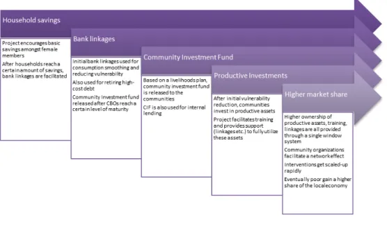
¹

Around 2008, a number of interventions meant to strengthen productive capacity and increase access to markets were added to the program: farmers were made familiar with sustainable low- input agricultural practices, procurement centers were opened, and milk cooperatives set up.

Efforts to enable poor people to benefit from government programs, such as pensions and scholarship, were also stepped up, and various social programs were initiated, such as nutrition centers for pregnant women and children. Figure 1 describes project interventions

schematically.

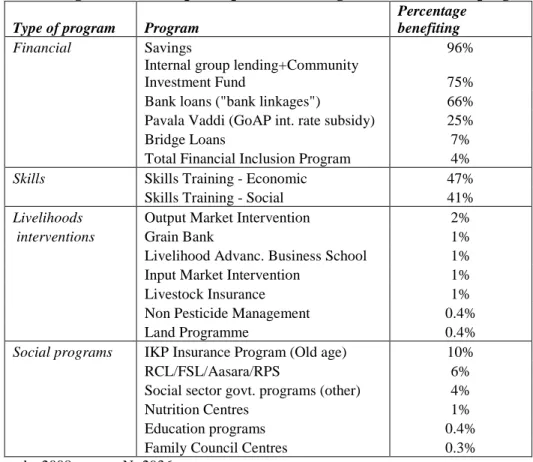
²

By 2008, most SHG members had benefited from interventions related to savings and credit and skills formation as well as linkages with government programs, while interventions to support productive investments and increased access to markets were not yet very widespread (Table 1).

Figure 1: Andhra Pradesh Indira Kranti Patham Economic Interventions

1 More details on the program can be found in World Bank (2003) and World Bank (2012).

2 See Kumara et al. (2009) on sustainable agriculture interventions and Shah and Chava (2012) on nutrition centers.

3

(6)

Table 1: Percentage of IKP SHG participants benefiting from various IKP programs, 2008

Type of program Program

Percentage benefiting

Financial Savings 96%

Internal group lending+Community

Investment Fund 75%

Bank loans ("bank linkages") 66%

Pavala Vaddi (GoAP int. rate subsidy) 25%

Bridge Loans 7%

Total Financial Inclusion Program 4%

Skills Skills Training - Economic 47%

Skills Training - Social 41%

Livelihoods Output Market Intervention 2%

interventions Grain Bank 1%

Livelihood Advanc. Business School 1%

Input Market Intervention 1%

Livestock Insurance 1%

Non Pesticide Management 0.4%

Land Programme 0.4%

Social programs IKP Insurance Program (Old age) 10%

RCL/FSL/Aasara/RPS 6%

Social sector govt. programs (other) 4%

Nutrition Centres 1%

Education programs 0.4%

Family Council Centres 0.3%

Note: Data from the 2008 survey. N=2936.

3. Data and descriptive statistics

The data for this study come from a panel survey conducted in 2004 and 2008 on a sample of about 4,250 households in 89 blocks in five districts of Andhra Pradesh.

³

Beyond district selection, which was done purposively to represent the state's five agro-climatic zones and average levels of economic, human, and infrastructure development, the sample was drawn randomly at the block, village, and household level.

⁴

In each village, 10 households were

3 The two surveys were respectively the baseline and end-line survey for the World Bank-supported Andhra Pradesh Rural Poverty Reduction Project (2003-2009, US$150 million). Attrition in the panel was limited: about 300 households visited in 2004 could not be re-interviewed in 2008 (a 6% attrition rate over the original 4,800). Another 250 households were discarded due to incomplete data, leaving us with about 4,250 households. A mid-term survey was also conducted in 2006, but has not been used it in this study because of data cleaning issues. The data were collected by the Centre for Economic and Social Studies in Hyderabad.

4 The five agro-climatic zones were North Coastal Andhra, South Coastal Andhra, Rayalseema, South Telangana and North Telangana. Levels of economic, human, and infrastructure development were assessed based on,

respectively, percentage of gross irrigated area, per capita income and percentage of urban population; percentage of SC, ST population, female literacy, infant mortality rates and percentage of children out of children (5-14 years);

total road length per 100 sq. km, number of banks per 10,000 people and number of hospital beds per 10,000 people.

The five districts selected (Kadapa, Nalgonda, Nellore, Visakhapatnam, and Warangal) ranked average in a composite index based on the indicators above. After selecting districts, 12 sub-district administrative units or blocks (called "mandals" in AP) were randomly selected in each district, and eight villages in each block, for a total

4

(7)

randomly selected from a list stratified by poverty category—poorest, poor, not-so-poor, and not poor—as determined through a survey- and community-based "participatory identification of the poor" exercise conducted in 2001. We exploit this categorization to disaggregate effects by poverty category, after correcting for the oversampling of the poorest and undersampling of the not-so-poor implied by the survey design (Table 2).

⁵

Table 2: Sample distribution by poverty category

Poverty category Observations Sample shares Weighted shares

Poorest 1,649 39 21

Poor 1,313 31 34

Not so poor 936 22 33

Not poor 361 8 12

4,259 100 100

The survey questionnaire, which was nearly identical in the two rounds, covered various outcome indictors, including expenditures on food and non-food items, assets (from consumer durables to farm and non-farm assets), land owned and operated, savings and loans, educational status, health status, household decision-making, autonomy, political participation. The data are of reasonably good quality.

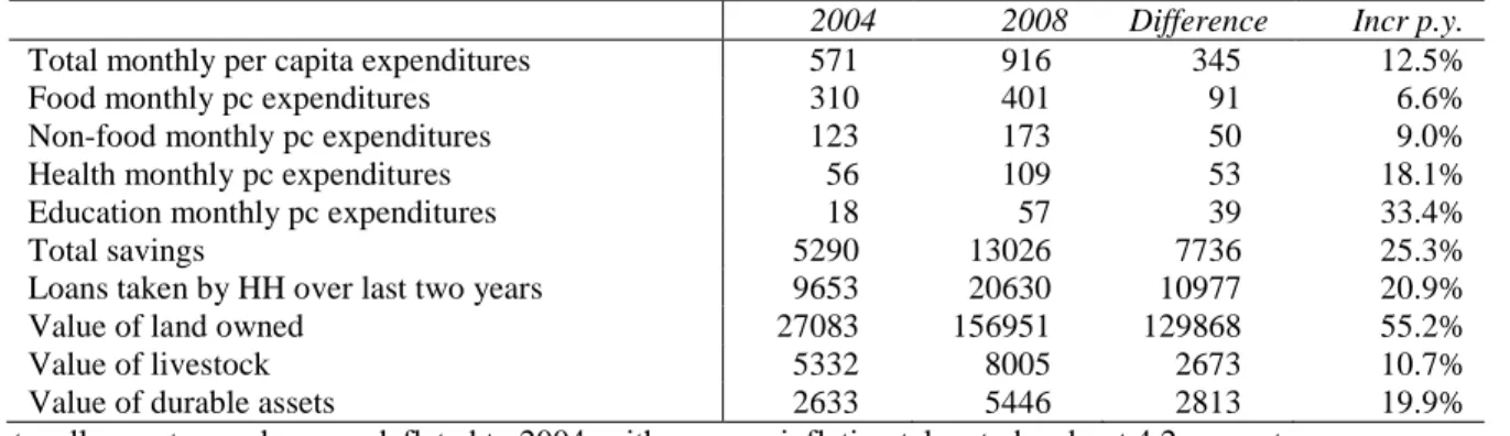
⁶

Sample means of key outcome indicators reveal sizable increases, which is not surprising given that the period 2004-2008 was one of rapid growth in AP (Table 3).

Table 3: Sample means of key outcome indicators (2004 Rs.)

2004 2008 Difference Incr p.y.

Total monthly per capita expenditures 571 916 345 12.5%

Food monthly pc expenditures 310 401 91 6.6%

Non-food monthly pc expenditures 123 173 50 9.0%

Health monthly pc expenditures 56 109 53 18.1%

Education monthly pc expenditures 18 57 39 33.4%

Total savings 5290 13026 7736 25.3%

Loans taken by HH over last two years 9653 20630 10977 20.9%

Value of land owned 27083 156951 129868 55.2%

Value of livestock 5332 8005 2673 10.7%

Value of durable assets 2633 5446 2813 19.9%

Note: all monetary values are deflated to 2004, with average inflation taken to be about 4.2 percent per year.

of 480 villages (only 11 blocks were covered in one district, but more villages were selected so as to have the same number of villages in each of the five districts). More details can be found in Galab and Reddy (2010).

5 The poorest of the poor were defined as those who could eat only when they got work and lacked shelter, proper clothing, social respect, and means to send their children to school; the poor as those having no land, living on daily wages, and needing to send school-age children to work in times of crisis. The ‘not-so-poor’ were defined as having some land, proper shelter, sending their children to public schools, being recognized in society, and having access to bank credit as well as public services. Those having more than 5 acres of land, no problem to obtain food, shelter, and clothing, hiring laborers, sending children to private schools, using private hospitals, lending rather than borrowing money, and having considerable social status were defined as non-poor (see Deininger and Liu (2013)).

Weights were constructed using block-level data from the participatory identification of the poor (PIP) exercise, as the village listing forms or PIP details are no longer available.

6 Questionnaires for 2008 were rechecked in the field for a small sample of households and found to be accurate. At the analysis stage, we checked some common indicators of data problems, such as the number of household

members or of food items consumed tapering off during fieldwork (to reduce workload), and did not find evidence of these issues. We also randomly checked household composition (number of members, gender, age, relationship to head) for the same household across surveys and found the data to be reasonably consistent.

5

(8)

In addition to IKP, households benefited from various government programs providing child care and nutrition, mid-day meals in schools, housing and sanitation, employment and other benefits (Table 4). Employment programs stand out, as their coverage grew tremendously with the introduction of the National Rural Employment Guarantee Scheme (NREGS) in 2006.

Table 4: Percentage of sample households benefiting from targeted government programs

2000 2003 2008

Self-Help Groups 20 44 71

Integrated Child Development Services 9 14 9

Midday meal and free hostels 8 29 27

Housing 14 6 19

Employment programs 0 9 41

Note: Data refer to May 2000 (based on recall), December 2003, and June 2008 as per the wording of the questionnaire. Self-Help Groups refers to DPIP in 2000-2003 and IKP afterwards. Midday meal and free hostels refers to hostels only in 2000, as the midday meal was introduced in Jan. 2003. Percentages for ICDS and midday meals/hostels refer to all households; for households with children of relevant ages, they are: ICDS: 22, 47, and 39 percent; midday meal/hostels: 13, 49, and 49 percent respectively. Employment refers to Food for Work in 2000- 2003 and NREGS in 2008.

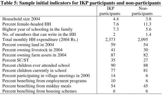
Households with members in the IKP Self-Help Groups (SHGs) in 2008 were better off in terms of initial household expenditures and education levels (Table 5), underscoring the need to carefully match participants and non-participants when assessing impacts.

Table 5: Sample initial indicators for IKP participants and non-participants

IKP

participants

Non- participants

Household size 2004 4.4 3.8

Percent female-headed HH 7.6 11.3

Highest year of schooling in the family 7.3 5.6

No. of members that can write in the HH 2 1.4

Total monthly HH expenditure (2004 Rs.) 2,373 2,095

Percent owning land in 2004 59 54

Percent owning livestock in 2004 41 30

Percent owning farm assets in 2004 87 82

Percent SC/ST 35 27

Percent children ever attended school 90 88

Percent children currently in school 77 81

Percent participating in village meetings in 2000 14 6

Percent benefiting from employment programs 10 6

Percent benefiting from midday meals 54 45

Percent benefiting from housing schemes 6 6

4. Empirical analysis

Impact evaluations aim to assess the impact of a program on a set of outcomes. We are

interested in how much outcomes changed for households participating in the program compared to households that did not participate. If Δ is the change in an outcome indicator for household i, we are interested in the difference between the change in the presence and the change in the absence of the program:

Program impact = E( Δ

i

/ P=1) - E( Δ

i

/ P=0) (1)

6

(9)

where P=1 denotes participation in the program and P=0 denotes no participation. But we do not observe outcomes for participating households in the absence of the program (the

"counterfactual"). Instead, we estimate the counterfactual by looking at the change for non- participants who are as much as possible similar to participants (the "control" group):

E( Δ

i

/ P=0) = E( Δ

i control

/P=0)

Estimated program impact = E( Δ

i

/ P=1) - E( Δ

i control

/P=0) (2) In randomized control trials, participants and non-participants are randomly selected from a pool of potential participants having similar characteristics. For the IKP evaluation, the intention was to randomly select mandals (blocks) where the program would be implemented and then

compare households in program mandals to households in non-program mandals. However, the control group was "contaminated": the program was extended to the control mandals much earlier than anticipated. Already by the time of the mid-term assessment in 2006 there were no control mandals left, and in 2008 we found essentially no differences between "program" and

"control" mandals: the shares of women in the sample villages who joined groups between 2004 and 2006 were slightly higher in "program" mandals (13 versus 10 percent on average) and the shares of women who joined between 2006 and 2008 slightly lower than in "control" mandals (15 versus 17 percent), but the average number of interventions from which program participants benefited was higher in "control" mandals (2.7 interventions in "program" mandals versus 2.9 in

"control" mandals). So the differences were negligible; there was no randomized placement of the intervention.

⁷

In the absence of randomization, we have to rely on Propensity Score Matching (PSM) to

construct a control group of non-participants with characteristics similar to those of participants.

PSM involves estimating the ex-ante probability of joining the program (called the "propensity score") as a function of a set of variables ("covariates") which influence program participation.

Studies comparing randomized control trial and non-experimental evaluations indicate that propensity score matching performs reasonably well when there is a rich set of data available from which to choose characteristics, the treatment and comparison groups are sampled using the same instruments, and the treatment and comparison groups come from similar geographic areas (see Smith and Todd (2001) and Diamond and Sekhon (2006)). Our data satisfy all three

criteria: we have a rich set of characteristics, the same survey instruments, and the two groups come from the same set of villages. We use nearest-neighbor matching with replacement as our main matching method, and check our results by using kernel matching.

We estimate propensity scores using a probit regression and include demographic, social, and economic characteristics as covariates:

⁸

whether the household has a female head, number of members, number of years of education of the most-educated family member, number of household members who can write, caste, expenditure levels, whether the household owned livestock, land, and assets. Including asset and land indicators among the covariates is

particularly important because of the perception among program implementers that, at least in the beginning, households that had some land were more likely to join, presumably because

7 Data on program coverage by mandal for 2004 and 2008 are not easily available, so we are unable to analyze outcomes using variation in coverage levels as a control.

8 Propensity scores estimated using a logit model are very similar, with differences below 0.1 percent.

7

(10)

landless households could see fewer benefits from microfinance and input/output procurement activities.

⁹

To control for unobservable personal characteristics, we also include an indicator of whether women in the household participated in community meetings at the village level (Panchayat Gram Sabha) in 2000, based on recall data, which we interpret as a proxy for initial empowerment levels.

¹⁰

We also include indicators of participation in government programs, specifically an employment and a school meal program, in 2004.

Since we are interested in looking at whether length of participation in group activities makes a difference, we consider three main comparisons, or "treatments":

• Households who had members in a group in 2004 and were still members in 2008 (early joiners) compared to households that never participated (i.e., at least four years of exposure to the program versus none)

• Households that joined during 2004-2006 (mid-joiners) compared to households that never participated (i.e., two to four years of exposure)

• Households that joined during 2007-2008 (late joiners) compared to households that never participated (i.e., less than two years of exposure).

We expect impacts to be higher for early and mid-joiners than for late joiners, as they would have participated in a wider range of activities and gained greater awareness of programs and services over time.

¹¹

Given the sampling design, we estimate propensity scores separately by poverty category (used as sub-classification, as suggested by Schuler, DuGoff, and Stuart, 2012). Table 6 describes the sample sizes for each comparison and poverty category. The 4,259 households for which we have full data include 161 households which were in the program in 2004 but dropped out later, which provide an interesting alternative "control" group.

¹²

While sample sizes are not huge, they are reasonable for each poverty category.

¹³

9 As time progressed, project staff made increasing efforts to reach all target households, so self-selection into the program became less of an issue over time. By 2008, however, the program had not reached all target households:

the percentage of poorest and poor households sampled who were group members ranged from 28 to 96 percent across blocks, with a third of all poorest and a fourth of all poor households sampled not in the program.

10 Results are very similar if we include in the propensity score matching regressions a woman's ability to set aside money for her own use, or whether she raised issues in Gram Sabha meetings, or a combination of these variables.

Using empowerment variables referring to 2003 also yields similar results.

11 Information on the number of activities each households benefited from by 2008 confirms that households with early and mid-joiners benefited from 4.1 activities compared to3.3 for late joiners.

12 Dropout households were slightly better off in terms of poverty category, caste, education, but not significantly different. They were of course different in that they decided the program was not useful to them—a feature we exploit later.

13 We group together not-so-poor and not poor under the label "not-so-poor".

8

(11)

Table 6: Sample size and weighted shares by treatment and poverty category

Poorest Poor

Not-so- poor +

not poor Total Poorest Poor

Not-so- poor +

not poor Total

Early 640 540 566 1,746 9 14 21 44

Mid 189 172 151 512 3 4 5 12

Late 235 220 223 678 3 6 7 16

Never 539 321 302 1,162 6 8 10 24

Dropouts 46 60 55 161 1 1 2 4

Total 1,649 1,313 1,297 4,259 21 34 44 100

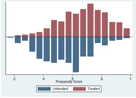
For each poverty category and comparison, we find non-participants with estimated probabilities of joining the program similar to those of participants across the probability distribution; in other words, there is sufficient overlap (or common support) in the estimated propensity scores to identify meaningful control groups. Figure 2 illustrates the propensity scores for poor early joiners and never joiners, while Table 7 reports and Figure 3 depicts the reduction in bias for each of the covariates used in matching. Balancing is reasonably good, with the absolute bias significantly reduced for most variables in all treatment/poverty category combinations.

¹⁴

Figure 2: Estimated propensity scores (early joiners vs. never joiners, poor households)

14 Tables and charts for the other treatment/poverty category combinations are available upon request. t-tests are not reported as they are not a reliable way of checking balance; see Austin (2009) and Stuart (2010) .

9

(12)

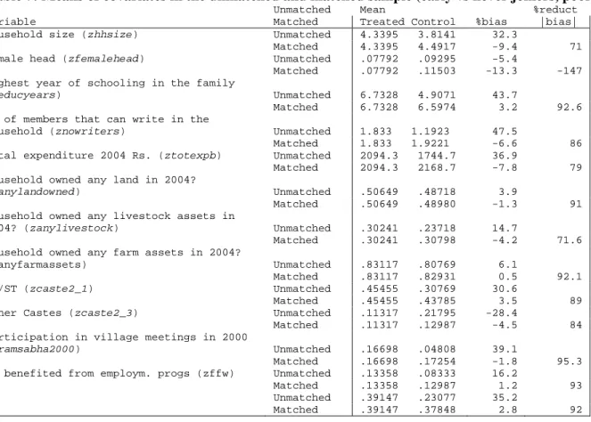
Table 7: Means of covariates in the unmatched and matched sample (early vs never joiners, poor)

Unmatched Mean %reduct

Variable Matched Treated Control %bias |bias|

Household size (zhhsize) Unmatched 4.3395 3.8141 32.3

Matched 4.3395 4.4917 -9.4 71 Female head (zfemalehead) Unmatched .07792 .09295 -5.4

Matched .07792 .11503 -13.3 -147 Highest year of schooling in the family

(zeducyears) Unmatched 6.7328 4.9071 43.7

Matched 6.7328 6.5974 3.2 92.6 No of members that can write in the

household (znowriters) Unmatched 1.833 1.1923 47.5

Matched 1.833 1.9221 -6.6 86 Total expenditure 2004 Rs. (ztotexpb) Unmatched 2094.3 1744.7 36.9

Matched 2094.3 2168.7 -7.8 79 Household owned any land in 2004?

(zanylandowned) Unmatched .50649 .48718 3.9

Matched .50649 .48980 -1.3 91 Household owned any livestock assets in

2004? (zanylivestock) Unmatched .30241 .23718 14.7

Matched .30241 .30798 -4.2 71.6 Household owned any farm assets in 2004?

(zanyfarmassets) Unmatched .83117 .80769 6.1

Matched .83117 .82931 0.5 92.1

SC/ST (zcaste2_1) Unmatched .45455 .30769 30.6

Matched .45455 .43785 3.5 89 Other Castes (zcaste2_3) Unmatched .11317 .21795 -28.4

Matched .11317 .12987 -4.5 84 Participation in village meetings in 2000

(gramsabha2000) Unmatched .16698 .04808 39.1

Matched .16698 .17254 -1.8 95.3 HH benefited from employm. progs (zffw) Unmatched .13358 .08333 16.2

Matched .13358 .12987 1.2 93 Unmatched .39147 .23077 35.2

Matched .39147 .37848 2.8 92

Figure 3: Reduction in bias for each covariate (early versus never joiners, poor households)

10

(13)

While propensity score matching controls for differences among participants and non-

participants that are correlated with observable characteristics (those used to estimate propensity scores), there may still be some unobserved characteristics that influence program participation and outcomes. The panel nature of our data allows us to also control for time-invariant

unobservable characteristics by taking the difference in the outcome of interest (for example expenditures) between 2004 and 2008 for each household before comparing between participants and non-participants ("difference-in-difference" or DID). Smith and Todd (2001) show that DID combined with propensity score matching yields the least biased results when compared to randomized control trial results.

¹⁵

The difference-in-difference approach assumes that expenditures and other outcomes of interest would have increased equally for participants and non-participants over the period in the absence of treatment; in other words, it assumes that outcomes display "equal trends in the absence of treatment".

¹⁶

If trends over time would have been different in the treatment and control groups, then the estimates of the impacts of the program would be biased. We test the validity of the

"equal trends" hypothesis by looking at trends over time in the three years preceding the baseline survey (2000-2003) for a few variables for which recall data on the earlier situation were

collected in 2004 and find that it holds.

Finally, following Abadie & Imbens (2009) and Stuart (2010) we use control variables in our regressions of DIDs over treatments for participants and matched non-participants to capture any residual effect and account for sampling design by using sampling weights in the regressions (as in Schuler, DuGoff, and Stuart, 2012). We control for female headship, indicators of

educational status, caste, participation in village meetings in 2003, and participation the most important government programs (employment, education, housing, see Table 4) in 2008.

5. Findings

5.a Borrowing, assets, and expenditures

Since greater savings and increased access to loans are the key benefits participants report they obtained from IKP during the period under study (see Table 1), it is reassuring to find that women who participated in groups were able to borrow up to two-and-a-half times more than non-participants, with higher amounts for poorest women who had been in groups longer (on average nearly Rs. 6,500 more over the two years prior to the survey).

¹⁷

Overall household borrowing was higher for participating households, indicating greater access to funds rather than just a substitution of female for male loans. Households were able to save a little more: poorest mid- and late-joiners, as well as poorest Scheduled Tribe (ST) early participants, had about Rs.

1,800 more savings than non-participants (Table A.1 reports DIDs, standard errors, absolute percentage changes for participants over non-participants, and number of observations for all poverty category and lengths of exposure).

15 See also the discussion in Voss (2008).

16 Gertler, Martinez, Premand, Rawlings, and Vermeersch (2011).

17 Because of the focus of IKP on microfinance, we consider savings and loans received in the two years preceding the survey despite all the known issues about the quality of survey data on financial balances (for example, we are unable to calculate outstanding loans and debt because we do not have information on all loans or on amounts still due).

11

(14)

The combination of social mobilization, skills training, savings and increased borrowing has translated into a higher increase into productive investments. The poorest households were able to operate a little more land (a quarter of an acre more for the poorest) and invested in livestock and durable assets (see Table A.2 and Table A.3). ST participants accumulated more livestock over non-participants than the average. Length of exposure did not make much of a difference, including for livestock, which is not surprising since acquiring livestock is commonly one of the first investments women make when they can access funds under IKP. Poor households also invested in land operated and livestock, but differences with non-participants, while positive, were generally not significant. They also invested in non-farm assets (such as means of transport) more than the poorest. Non-poor participants bought more land. The fact that only non-poor participants showed significant differences in land owned may point to the difficulties poorest and poor households experience in acquiring land and provide a rationale for the efforts made in recent years by IKP to facilitate land titling for the poorest.

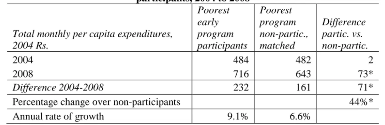
Increased availability of funds also translated into greater spending on education for poorest and poor households, across lengths of exposure. Effects on total and food expenditures were more muted. Poorest participants were able to spend more than non-participants, but generally not significantly so. To illustrate, in 2004, total monthly per capita expenditures were Rs. 484 for the poorest early joiners and Rs. 482 for matched non-participants (this small difference is by design, since total expenditures are included in the matching algorithm). In 2008, expenditures were Rs. 716 and Rs. 643 respectively (in 2004 prices). Thus, poorest participants saw an increase of Rs. 232 against Rs. 161 for non-participants—an additional gain (or DID) of Rs. 71, or 44 percent more than non-participants (our counterfactual) (Table 8).

Table 8: Changes in total monthly pc expenditures for poorest early joiners and matched non- participants, 2004 to 2008

Total monthly per capita expenditures, 2004 Rs.

Poorest early program participants

Poorest program non-partic., matched

Difference partic. vs.

non-partic.

2004 484 482 2

2008 716 643 73*

Difference 2004-2008 232 161 71*

Percentage change over non-participants 44%*

Annual rate of growth 9.1% 6.6%

Note:

nearest neighbor propensity score matching, regression-adjusted, with survey weights.

This additional total monthly per capita expenditure (Rs. 71) is 24 percent of the 2004-05 rural poverty line for Andhra Pradesh, which was Rs 293 monthly per capita (Government of India, 2007).

¹⁸

Total monthly per capita expenditures grew at an annual rate of more than 9 percent for the poorest participants versus 6.6 percent for non-participants. So the gain for participants over non-participants is not huge but not insignificant either.

18 We use the old poverty lines, not the Tendulkar lines, since we refer to 2004. Note that our poorest households had 2004 expenditure levels well above the poverty line, while being defined as "poorest"--on average Rs. 455 monthly per capita. This discrepancy warrants further investigation.

12

(15)

Consistent with the focus of IKP on the most marginalized, differences were quite large for ST participants; Table 9 replicates the results above for STs only, indicating an additional gain of 187 percent over ST non-participants (and the gain is significant despite a small sample size).

Table 9: Changes in total monthly pc expenditures for poorest early joiners and matched non- participants, Scheduled Tribes, 2004 to 2008

Total monthly per capita expenditures, 2004 Rs.

Poorest early program ST participants

Poorest program ST non-partic., matched

Difference ST partic.

vs. non- partic.

2004 347 375 28

2008 543 443 100

Difference 2004-2008 196 68 128*

Percentage change over non-participants 187%*

Annual rate of growth 10.4% 3.8%

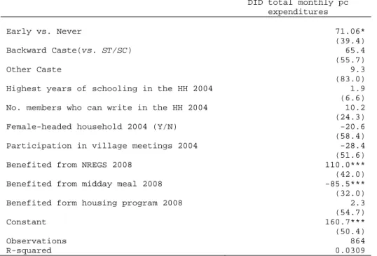
Table 10 illustrates how we control for any remaining impact of other factors in the regressions, referring to the case in Table 8. Female headship decreases expenditures per capita while higher education levels have a positive impact, but none of the controls that were also included in the matching are significant, as expected, indicating that their effects on expenditures have been captured through the propensity score matching process.

Table 10: Impact of the program on DID for total monthly per capita expenditures, early versus never joiners, poorest households

¹⁹

DID total monthly pc expenditures

Early vs. Never 71.06*

(39.4)

Backward Caste(vs. ST/SC) 65.4

(55.7)

Other Caste 9.3

(83.0) Highest years of schooling in the HH 2004 1.9 (6.6) No. members who can write in the HH 2004 10.2 (24.3)

Female-headed household 2004 (Y/N) -20.6

(58.4)

Participation in village meetings 2004 -28.4

(51.6)

Benefited from NREGS 2008 110.0***

(42.0)

Benefited from midday meal 2008 -85.5***

(32.0)

Benefited form housing program 2008 2.3

(54.7)

Constant 160.7***

(50.4)

Observations 864

R-squared 0.0309

Note: Robust standard errors in parentheses. Significance levels: *: 10 percent, **: 5 percent, ***: 1 percent.

19 The number of observations in the table is lower than the total sample size, because nearest-neighbor matching excludes control observations that are not "nearest" a treated observation. While this "loss" of observations may appear undesirable as it may reduce power, in fact this effect is often minimal, as precision is higher when the two groups being compared are more similar (Stuart 2010).

13

(16)

What has a significant positive impact, however, is participation in the National Rural

Employment Guarantee Scheme (NREGS), launched in 2006. So are the impacts due to IKP or to NREGS? Disentangling IKP and NREGS effects is complex: IKP influences NREGS

participation, as we will see below, and NREGS participation enhances income and

expenditures. Essentially, NREGS indeed contributes to the changes in expenditures for IKP participants, but so does IKP.

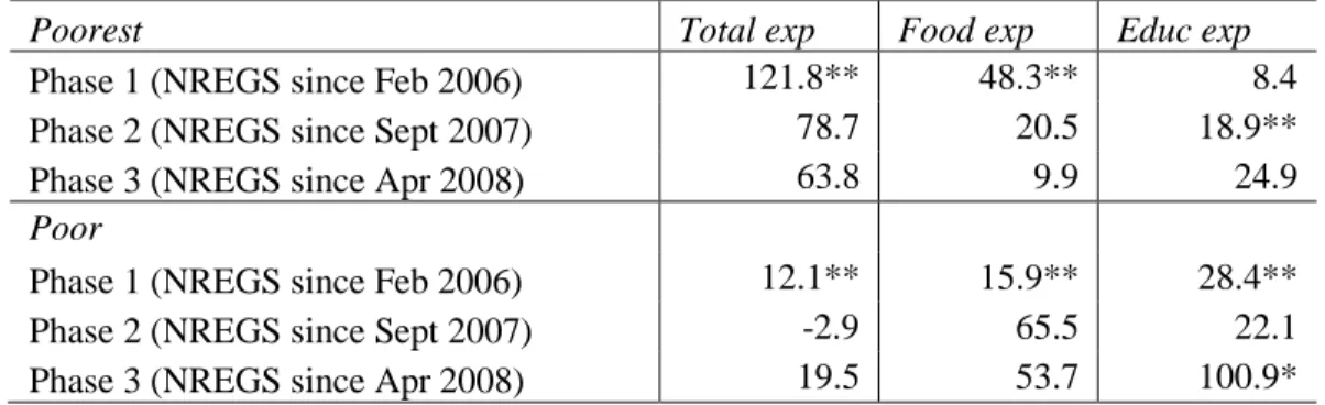
To see this, we check whether IKP had an impact where NREGS was not relevant. First, we exploit the fact that NREGS was expanded across survey districts in phases. Table 11 presents total, food, and education expenditure DIDs for poorest and poor households in districts where NREGS started in February 2006 (Phase 1), September 2007 (Phase 2), and April 2008

(Phase 3). The DIDs for total expenditures for poorest households were higher where NREGS had been active longer: Rs. 122 in Phase 1 districts, Rs. 79 in Phase 2, but still a positive if not significant Rs. 64 in Phase 3 districts, where NREGS had been operating for a few months at most at the time of the 2008 survey. The DID for education expenditures were significantly positive for some categories also where NREGS had been operating for shorter lengths of time.

Table 11: DIDs for monthly per capita expenditures, early vs. never joiners, by NREGS phasing, 2004 Rs.

Poorest Total exp Food exp Educ exp

Phase 1 (NREGS since Feb 2006) 121.8 48.3 8.4

Phase 2 (NREGS since Sept 2007) 78.7 20.5 18.9**

Phase 3 (NREGS since Apr 2008) 63.8 9.9 24.9

Poor

Phase 1 (NREGS since Feb 2006) 12.1 15.9 28.4**

Phase 2 (NREGS since Sept 2007) -2.9 65.5 22.1

Phase 3 (NREGS since Apr 2008) 19.5 53.7 100.9*

Note: Significance levels: *: 10 percent, **: 5 percent, ***: 1 percent.

Another way to isolate the impact of IKP is to look at DIDs separately who did and did not benefit from NREGS. Among those who benefited from NREGS, IKP participants had positive expenditure DIDs, significant for education; among those who did not benefit, DID are still positive for poorest participants, if not significant, and education spending is significant for poor households. Thus, IKP appears to have had a direct positive impact for the poorest and for education expenditures over and above the impact of NREGS.

Table 12: DIDs for monthly per capita expenditures, early joiners vs. never joiners, by NREGS participation, 2004 Rs.

Total exp Food exp Educ exp Poorest

Households benefiting from NREGS 68 33 39*

Households not benefiting from NREGS 50 10 11

Poor

Households benefiting from NREGS 157 20 38

Households not benefiting from NREGS -40.6 -13.6 12.2**

14

(17)

5.b Participation in government programs

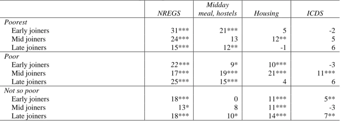
As mentioned, the interaction of IKP and NREGS is complex. Did IKP affect the likelihood that a household benefit from NREGS? Our data point to a strong correlation between membership in IKP and benefiting from NREGS: across all poverty categories and lengths of exposure, IKP participants were significantly more likely to report benefiting from NREGS. Not only, but poorest and poor IKP participants were also significantly more likely to report benefiting from midday meals and student hostel schemes. Poor and not so poor participants were more likely than non-participants to benefit from housing schemes (Table 13). IKP clearly facilitated participation in these key government programs in a major way. The correlation with benefiting from ICDS, access to which was not stressed under IKP, is not so strong.

Table 13: Additional probability of benefiting from NREGS and other programs for IKP participants, 2008

NREGS

Midday

meal, hostels Housing ICDS Poorest

Early joiners 31*** 21*** 5 -2

Mid joiners 24*** 13 12** 5

Late joiners 15*** 12** -1 6

Poor

Early joiners 22*** 9* 10*** -3

Mid joiners 17*** 19*** 21*** 11***

Late joiners 25*** 15*** 4 6

Not so poor

Early joiners 18*** 0 11*** 5**

Mid joiners 13* 8 11*** -3

Late joiners 18*** 10* 14*** 7**

5.c Human development indicators

Next, we turn to education and health indicators. Education indicators are generally better in AP than in northern Indian states, and the data confirm that most children attended at least some school. Enrollment rates increased for all, but differences were not significant in either 2004 or 2008. Current school attendance increased slightly for children of IKP participants (all lengths of exposure taken together), and actually appears to have declined for children of non-

participants (Table 14). The increase in current attendance is largest for children of longest IKP participants, including the poorest (Table A.5).

Table 14: Percentage of school-age children who attended at least some school and who were currently in school

All children who ever attended Female children who ever attended IKP

particip

Non-partic Difference partic. vs.

non-partic.

IKP particip

non-partic.

2003 81 82 -1 81 80 0

2008 84 85 -1 81 80 0

Diff. over time 3 3 0 0 0 0

15

(18)

All children who were currently attending

IKP particip

non-partic.

2003 69 72 -3

2008 70 64 6

Diff. over time 1 -8 9*

Note: Significance levels: *: 10 percent, **: 5 percent, ***: 1 percent. The data refer to households who had children in school in both periods, all poverty categories and lengths of exposure combined, with regression adjustments; detailed results are in Table A.5.

Here too, though, we need to disentangle the effects of IKP from those of the midday meal program, which continued to provide an important incentive to attend school during the period under study. To do so, we look at current attendance in households that report not benefiting from the midday meal in 2008 (almost half the households with children in school) and we find that the decline was significantly smaller for children of IKP participants. We also find a very significant increase in children currently attending school among households that report benefiting from the midday meal, IKP participants and non-participants, confirming the importance of the program (Table 15).

Table 15: Percentage of school-age children who were currently in school, by reported benefits from the midday meal program

All children who were currently attending but not benefiting from

midday meal in 2008

All children who were currently attending and benefiting from midday

meal in 2008 IKP

particip

non-partic.

IKP particip

non-partic.

2003 70 75 -5* 74 75 -1

2008 63 56 7 96 94 2

Diff. over time -7 -19 12** 22 19 3

Note: Significance levels: *: 10 percent, **: 5 percent, ***: 1 percent. The data refer to households who had children in school in both periods, all poverty categories and lengths of exposure combined.

In sum, the additional investment in education by IKP members observed earlier appears to have translated into more children staying in school, particularly for the poorest, where the midday meal program was not functioning well.

On health, we find some signs of improvement but many more areas of concern. On the positive side, the percentage of births over the two years prior to the survey that took place at a facility or were assisted by a trained birth assistant increased, in both participant and non-participant households. On the other hand, immunization cards declined for participants and exclusive breastfeeding declined for all, but particularly among IKP participants (Table 16).

Table 16: Incidence of assisted deliveries, exclusive breastfeeding, presence of immunization cards

Assisted delivery

IKP particip

non-partic.

2003 76 75 1

16

(19)

2008 85 82 2

Diff. over time 9 7 2

Immunization cards Breastfeeding

IKP particip

non-partic.

IKP particip

non-partic.

2003 90 87 3 86 92 -6

2008 88 96 -8*** 83 92 -9***

Diff. over time -2 9 -11 -3 0 -3

Note: The data refer to households that had deliveries or small children in the two years prior to each survey. The results are for all poverty categories and lengths of exposure combined, with regression adjustments. Because the number of HH who had children in both periods is small, we do not calculate differences-in-differences.

Indicators of maternal and child health do not show much improvement either. Knowledge of diarrhea treatment increased marginally; knowledge of modern contraceptive methods increased but still no more than a fifth of all women had knowledge about modern contraceptive methods;

and the percentage of women visited by Family Planning workers actually declined (Table 17).

None of the differences between participants and non-participants are significant, nor are there meaningful differences by length of exposure or poverty category (not reported).

Table 17: Knowledge of diarrhea treatment and family planning, FP worker visits

Diarrhea treatment Modern methods

IKP particip

Non- partic

Difference partic. vs.

non- partic.

IKP particip

Non- partic

non- partic.

2003 41 37 4 5 9 -4

2008 45 43 2 22 24 -2

Diff. over time 4 6 2 17 15 2

FP visit IKP

particip

Non- partic

non- partic.

2003 79 77 2

2008 60 53 7*

Diff. over time -19 -24 5

Note: The data refer to households that responded in both surveys. The results are for all poverty categories and lengths of exposure combined, with regression adjustments.

Virtually all indicators moved similarly for participants and non-participants. This is perhaps not surprising, as there were essentially no health-related interventions under IKP up to 2008. But the findings do suggest that the strong focus placed by the program, beginning in 2007, on

17

(20)

nutrition and maternal and child health through the Nutrition cum-Day Care Centers was well justified.

²⁰

5.d Empowerment

Next, we look at the impact of membership in groups on women's empowerment. Empowerment has been defined as "the expansion of people's ability to make strategic life choices in a context where this ability was previously denied to them" (Kabeer, 1999). The survey allows us to look at women's autonomy, mobility, and participation in social activities. Information was collected for 2003 and 2006-08 and, by recall, for 2000.

²¹

First, we consider women's ability to set money aside for their own use and find that slightly more women were able to do so always or frequently in 2008 than earlier, both IKP participants and non-participants, with no significant differences (Table 18), apart from not-so-poor early joiners, who were able to set aside money more frequently, probably as a reflection of greater availability of money (not reported).

Table 18: Percentage of women able to set some money aside for personal use

Able to set aside some money for own use

IKP participants

Non- participants

non-partic.

2000 33 33 0

2003 32 32 0

2008 36 36 0

Note: Results for all poverty categories and lengths of exposure combined.

Second, we look at whether women were afraid to disagree with their husbands. Here, we find a significant impact of IKP participation. Over time, all women became less afraid to disagree (especially the poor and not-so-poor), with IKP participants significantly less afraid.

Table 19: Percentage of women not afraid to disagree with their husbands

Women not afraid to disagree with their

husbands IKP participants

non-partic.

2000 79 71 8***

2003 81 73 8***

2008 84 80 4**

20 By 2008, less than 1% of households surveyed had benefited from a Nutrition Center, so it was too early to detect any impacts.

21 While the survey also asked whether decisions on major events—children's education and marriage, purchase of property and durable goods, savings, health care and family planning—if faced, were taken by the husband, the wife, or jointly, these major decisions are faced only infrequently and sample sizes are too small for meaningful analysis. The reference time periods were up to May 2000, Jan-June 2003, and July 2006-June 2008. Because of the ordinal nature of the data (with ratings such as "always", "sometimes", "rarely", etc.), we generally do not construct differences-in-differences, but look at levels over time using propensity score matching and regression adjustments, unless otherwise specified.

18

(21)

Note: Results for all poverty categories and lengths of exposure combined. Significance levels: *: 10 percent, **: 5 percent, ***: 1 percent.

Next, we look at women's ability to visit people and places without their husband's or other family member's permission, and find a sizable increase in this dimension of autonomy.

²²

Still, women's mobility was far from unrestricted: less than half could visit the community center or attend community functions without getting permission first (Table 20).

Table 20: Percentage of women who can go out alone without permission, 2008

IKP

participants

non-partic.

To the market 75 72 3

To visit friends 68 62 6*

To visit relatives 61 52 9***

To the local health center 72 65 7**

To fields outside the village for work 48 42 6*

To the community center/park/plaza in the village 44 38 6*

To community functions 36 31 5*

Note: Results for all poverty categories and lengths of exposure combined. Significance levels: *: 10 percent, **: 5 percent, ***: 1 percent.

By poverty category, differences are largest for not-so-poor women, whose mobility is restricted more than that of poorer women. Non-poor IKP participants were 10 percent more likely to be able to visit relatives or go to the health center alone than similar non-participants (Table 21). In 2003, the differences between members and non-members were not significant (not reported), confirming the positive impact of IKP on the mobility of better-off women.

Table 21: Percentage of not-so-poor women who can go out alone without permission, 2008

IKP

participants

non-partic.

To the market 65 59 6

To visit friends 58 51 7

To visit relatives 67 57 10**

To the local health center 78 67 11**

To fields outside the village for work 51 46 5 To the community center/park/plaza in the village 44 39 5

To community functions 31 31 0

Note: Results for not-so-poor women, all lengths of exposure combined. Significance levels: *: 10 percent, **: 5 percent, ***: 1 percent.

In addition to looking at various dimensions separately, we construct an index (as done for instance by Bali Swain and Wallentin (2012) and Deininger and Liu (2012a)).

²³

Following Kolenikov and Angeles (2004) and Bali Swain and Wallentin (2012), we use principal

22 Unfortunately, there was a change in coding on the mobility variables between 2004 and 2008; we observe improvements under different ways of matching old and new codes.

23 We use going to the market, visiting friends and relatives, attending community functions, setting money aside, and disagreeing with husbands; other indicators have many missing answers and would cause us to lose too many observations.

19

(22)

component analysis to identify the latent autonomy variable and rely on polychoric correlations to address the ordinal nature of the data. We find higher values of the empowerment index for IKP participants than non-participants and an increase over time, but the difference in the change over time is not significant and in fact the index rose slightly faster for non-participants.

Finally, we look at women's participation in village meetings, namely Gram Sabhas at the Panchayat (village) level. Attending village meetings may require going to a different, often higher-caste hamlet and it is not common among women. Simple sample means indicated large differences between IKP participants and non-participants even before the program started, justifying the inclusion of participation in village meetings in the matching algorithm and in regression controls (refer to Table 5). Even after matching and controlling for initial propensity to participate, IKP participants were 4% more likely to attend village gram sabhas in 2008, with the effect concentrated among women who had participated in the program longest (Table 22) and among poor and not-so-poor women (not shown).

Table 22: Percentage participating in village meetings always or frequently, 2008

IKP

participants

non- partic.

Early joiners

¹⁶ ⁸ ^8***

Mid joiners

¹¹ ⁹ ²

Late joiners

⁸ ¹⁰ ^-2

Ever joiners

¹⁴ ¹⁰ ^4**

Note: All poverty categories combined. Significance levels: *: 10 percent, **: 5 percent, ***: 1 percent.

To summarize, we see general improvements over time in women's ability to go out without permission and to disagree with husbands, and we find that IKP enabled women members to achieve greater autonomy and participate in village meetings over and above the general trend.

Since we do not have observations from non-program villages, we cannot ascertain whether the IKP was responsible for the general improvements we observe, by changing norms of what is socially acceptable, for both participants and non-participants.

6. Robustness of the estimates

6.a Comparison group

We carry out a number of sensitivity analyses to check our results. First, we exploit the presence in the sample of a small group of households who were in the program in 2004 but dropped out by 2008 (the "dropouts" in Table 6). These were "early joiners" in the sense that they were group members in 2004 (having joined on average at the same time as early joiners) and

presumably expected ex ante to receive benefits from the program, like those who stayed in. So we can take the evolution over time of their indicators as a proxy for what would have happened to early joiners if they had not been in the IKP during 2004-2008. DIDs for female and total loans, land owned, education expenditures, and girl children who ever attended school remain positive and significant.

20

(23)

6.b Model specification

We also check results across model specifications. The tables below report degrees of significance of estimates of DIDs for early and mid-joiners under two specifications of the propensity score matching algorithm (nearest neighbor and kernel) and two options for

regressions (weighted using survey weights and unweighted). We report results for a selection of indicators: savings, female loans, and household loans in Table 23; livestock, non-farm, and durable asset values in Table 24; total, food, and education expenditures in Table 25, and school attendance and enrollment in Table 26.

As expected, both the size of effects and the degree of significance vary, but signs, orders of magnitude, and significance are generally similar across specifications. In addition to female and total loans, the DIDs which are most consistently significant across specifications are those for livestock and durable goods for the poorest and non-farm assets for the poor. DIDs for savings for poorest and poor, total expenditures for the poorest early joiners, and education expenditures for poorest and poor also remain significant across several specifications. DIDs for food expenditures and for education outcomes, on the other hand, are not significantly different between participants and non-participants whatever model specification we choose. Looking at estimated values, the DID for total expenditures (the additional gain) for poorest early joiners ranges from range from Rs. 34 to Rs. 71, or 15 to 44% more than for non-participants, with our preferred specification (nearest-neighbor propensity score matching with sampling weights in the regressions, Table 8) falling at the high end of the range.

Table 23: Significance of DIDs for savings and loans under various model specifications

²⁴ Savings NN no SW Ker no

SW NN SW Ker SW

Poorest Early vs. Never - + + +

Poorest Mid vs. Never +** + +** +

Poor Early vs. Never +** +* +** +*

Poor Mid vs. Never + + + +

Non-poor Early vs. Never - - - -

Non-poor Mid vs. Never - - - -

Loans previous two years female NN no SW

Ker no

SW NN SW Ker SW

Poorest Early vs. Never +*** +*** +*** +***

Poorest Mid vs. Never +*** +*** +*** +***

Poor Early vs. Never +*** +*** +*** +***

Poor Mid vs. Never +*** +*** +*** +***

Non-poor Early vs. Never + +** +** +**

Non-poor Mid vs. Never +*** +*** +*** +***

24 NN no SW=Nearest-neighbor propensity score matching, regressions without survey weights. Ker no SW=Kernel propensity score matching, regressions without survey weights. NN SW=Nearest-neighbor propensity score matching, regressions with survey weights. Ker SW=Kernel propensity score matching, regressions with survey weights.

21

(24)

Loans previous two years total NN no SW

Ker no

SW NN SW Ker SW

Poorest Early vs. Never +*** +*** +*** +***

Poorest Mid vs. Never + +** + +

Poor Early vs. Never + +* + +

Poor Mid vs. Never +*** +*** +*** +**

Non-poor Early vs. Never + +* +* +**

Non-poor Mid vs. Never + + + +

Table 24: Significance of DIDs for assets under various model specifications

Value of all livestock assets NN no

SW

Ker no SW

NN SW

Ker SW Poorest Early vs. Never +*** +*** +*** +***

Poorest Mid vs. Never +*** +** +*** +***

Poor Early vs. Never + + + +

Non-poor Early vs. Never + + + -

Value of non-farm assets NN no SW

Ker no SW

NN SW

Ker SW

Poorest Early vs. Never + + + -

Poorest Mid vs. Never - - - -

Poor Early vs. Never + +* + +**

Poor Mid vs. Never +** +** +** +**

Non-poor Mid vs. Never - -* - -*

Value of durable assets NN no SW

Ker no SW

NN SW

Ker SW Poorest Early vs. Never +** +*** +** +***

Poorest Mid vs. Never +*** +* + +

Poor Mid vs. Never + +* + +

Non-poor Early vs. Never + + - -

Table 25: Significance of DIDs for expenditures under different model specifications

Total expenditures per

capita NN no SW Ker no SW NN SW Ker SW

Poorest Early vs. Never +* + +* +

Poorest Mid vs. Never - -* - -

Poor Mid vs. Never +* +** +** +**

Non-poor Early vs. Never + - - -

22

(25)

Food expenditures per

capita NN no SW Ker no SW NN SW Ker SW

Poorest Early vs. Never + + + +

Poorest Mid vs. Never - - + +

Poor Early vs. Never - - - -

Education exp pc NN no SW Ker no SW NN SW Ker SW

Poorest Early vs. Never + + + +**

Poorest Mid vs. Never + + +** +*

Poor Early vs. Never + + + +**

Poor Mid vs. Never +* +* +** +**

Non-poor Early vs. Never + + + +

Table 26: Significance of DIDs for school attendance and enrollment under different model specifications

All children who ever attended NN no SW

Ker no

SW NN SW Ker SW

Poorest Mid vs. Never + + + +

Poor Mid vs. Never + - + -

Non-poor Early vs. Never + - + -

Non-poor Mid vs. Never - - - +

Female children who ever attended

Poorest Mid vs. Never + + - -

Poor Early vs. Never - - - -

Poor Mid vs. Never - - -

Non-poor Early vs. Never + + + +

Non-poor Mid vs. Never - + + +

All children who were currently

attending

Poorest Early vs. Never +* + +** +

Poorest Mid vs. Never + + - -

Poor Early vs. Never +* + + +

Non-poor Early vs. Never + + + -

Non-poor Mid vs. Never + + + +**