Hartz IV and the Decline of German Unemployment: A Macroeconomic Evaluation

IHS Working Paper 31

March 2021

Hartz IV and the Decline of German Unemployment: A Macroeconomic Evaluation

Brigitte Hochmuth

Britta Kohlbrecher

Christian Merkl

Hermann Gartner

Author(s)

Brigitte Hochmuth, Britta Kohlbrecher, Christian Merkl, Hermann Gartner Editor(s)

Robert M. Kunst Title

Hartz IV and the Decline of German Unemployment: A Macroeconomic Evaluation

Institut für Höhere Studien - Institute for Advanced Studies (IHS) Josefstädter Straße 39, A-1080 Wien

T +43 1 59991-0 F +43 1 59991-555 www.ihs.ac.at ZVR: 066207973 Funder(s)

DFG (grant number ME-3887/5-1), Hans-Frisch-Stiftung License

„Hartz IV and the Decline of German Unemployment: A Macroeconomic Evaluation “ by Brigitte Hochmuth, Britta Kohlbrecher, Christian Merkl, Hermann Gartner is licensed under the Creative Commons: Attribution 4.0 License

(http://creativecommons.org/licenses/by/4.0/)

All contents are without guarantee. Any liability of the contributors of the IHS from the content of this work is excluded.

All IHS Working Papers are available online:

https://irihs.ihs.ac.at/view/ihs_series/ser=5Fihswps.html

This paper is available for download without charge at: https://irihs.ihs.ac.at/id/eprint/5705/

Hartz IV and the Decline of German

Unemployment: A Macroeconomic Evaluation ^†

Brigitte Hochmuth ^1,2 , Britta Kohlbrecher ¹ , Christian Merkl ^1,3 , and Hermann Gartner ^1,4

1 Friedrich-Alexander University of Erlangen-Nürnberg (FAU)

2 Institute for Advanced Studies Vienna (IHS)

3 IZA

4 Institute for Employment Research (IAB)

March 3, 2021

Abstract

This paper proposes a new approach to evaluate the macroeconomic effects of the

“Hartz IV” reform, which reduced the generosity of long-term unemployment benefits.

We propose a model with different unemployment durations, where the reform initiates both a partial effect and an equilibrium effect. We estimate the relative importance of these two effects and the size of the partial effect based on the IAB Job Vacancy Survey.

Our approach does not hinge on an external source for the decline in the replacement rate for long-term unemployed. We find that Hartz IV was a major driver for the decline of Germany’s steady state unemployment and that partial and equilibrium effect were nearly of equal importance. In addition, we provide direct empirical evidence on labor selection, one potential dimension of recruiting intensity.

JEL classification: E24, E00, E60.

Keywords: Unemployment benefits reform, search and matching, Hartz reforms

†

We are grateful for feedback at the following conferences: CESifo Conference on Macroeconomics and Survey Data (Munich), Ensuring Economics and Employment Stability (Nuremberg), T2M 2018 (Paris), Verein für Socialpolitik 2019 (Leipzig) and the Austrian Labor Market Workshop 2019 (Vienna). We have obtained very useful feedback at seminars at Australian National University, Humboldt Universität, IAB, IMK, International Monetary Fund, IWH Halle, OECD, University of Strasbourg, University of Adelaide, University of Bamberg, University of Trier and the University of Queensland. We would like to thank Vincent Sterk for an insightful discussion of our paper and are grateful for feedback from Leo Kaas, Andrey Launov, Kurt Mitman, Mathias Trabandt, and Coen Teulings. We are grateful for funding from the German Research Foundation (DFG) with grant number ME-3887/5-1 and the Hans- Frisch-Stiftung.

e-mail: christian.merkl@fau.de.

1 Introduction

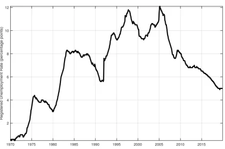
Since the implementation of an unemployment benefits reform in the year 2005 (dubbed as

“Hartz IV”), which reduced the average benefit replacement rate for long-term unemployed, the German unemployment rate has declined from 12 percent in 2005 to 5 percent in 2019 (see Fig- ure 1). The existing literature has not yet reached a consensus on how much the Hartz IV re- form has contributed to this decline. On the one hand, there are microeconometric studies (in particular, Price, 2019) that show a significant increase of the unemployment-to-employment transition rate for those close to the expiration of short-term unemployment benefits. However, these studies remain silent about the potential equilibrium effects of the reform. On the other hand, quantitative results in macroeconomic models of the labor market depend strongly on the assumed reduction of the replacement rate for long-term unemployed. However, because of the complex structure of the unemployment benefit system, there is no consensus on the overall reduction of the replacement rate (see Section 2). Due to different assigned values for the reduc- tion of the replacement rate, the quantitative unemployment effects in existing macroeconomic studies (Krause and Uhlig, 2012, Krebs and Scheffel, 2013, Launov and Wälde, 2013) range from close to zero to a 2.8 percentage point reduction of steady state unemployment.

Figure 1: Registered unemployment rate in Germany, 1970-2019.

1970 1975 1980 1985 1990 1995 2000 2005 2010 2015

2 4 6 8 10 12

Registered Unemployment Rate (percentage points)

Our paper offers a solution to this disagreement. We propose a labor market model with a rich unemployment duration structure. In our model, hiring is a two-stage process where firms have to establish a contact and select a certain fraction of workers. A benefit reform triggers two ef- fects. First, it stimulates vacancy posting, thereby increases market tightness and aggregate con- tacts between workers and firms. We call this the equilibrium effect. Second, firms select a larger fraction of workers (i.e. they are less selective), which we call the partial effect. We can measure this worker-firm-level effect directly in the data. For this purpose, we propose a new proxy for the selectivity of firms based on the IAB Job Vacancy Survey and estimate the increase of the se- lection rate (share of selected suitable applicants) due to Hartz IV. ¹ In addition, we use the IAB

1

Descriptively, the selection rate increased from 46 percent (1992-2004) before the Hartz IV reform to 53 percent

Job Vacancy Survey to estimate the relative importance of partial and equilibrium effects over the business cycle, which we find to be equally important. The estimation results discipline the partial and the equilibrium effect in our macroeconomic model of the labor market. Our quan- titative exercise yields a 2.1 percentage point decline of unemployment. This strategy replaces the conventional approach to assume a certain decline of the replacement rate, which is based on an exogenous source.

We validate our model along three dimensions (see Appendix C for details). First, the time se- ries properties of our model are in line with the data in various dimensions. Second, our partial effects are similar to the causal microeconometric results from Price (2019). Third, there is sup- portive evidence for our simulated aggregate outcomes. The aggregate unemployment effects are in line with time series evidence by Klein and Schiman (2021). In addition, consonant with descriptive evidence, the job-finding rate for short-term unemployed reacts more strongly than for long-term unemployed. Furthermore, the model-based Beveridge Curve movement in re- sponse to the Hartz IV reform is similar to the actual movement of the Beveridge Curve in the years after the reform. ²

Our model combines three ingredients: First, workers and firms meet randomly. Meetings are driven by a Cobb-Douglas constant returns contact function (Mortensen and Pissarides, 1994). ³ Second, upon meeting, only a certain fraction of contacts is hired. All meetings draw an idiosyn- cratic training cost shock from a stable density function (see Chugh and Merkl, 2016 or Sedlá˘cek, 2014). Firms only select workers with an expected positive present value. Third, as Hartz IV was a reform of long-term unemployment benefits, we model a detailed deterministic unemployment structure. In our model, less generous long-term unemployment benefits trigger two effects.

First, vacancy posting is stimulated (due to lower negotiated wages) and thereby the probability of making a contact with a firm increases for all workers. This equilibrium effect would not be measured in microeconometric studies. Second, less generous long-term unemployment ben- efits will affect the surplus of employment relative to unemployment. Due to this higher joint surplus, a larger fraction of applicants will be selected by firms upon meeting (partial effect).

Our paper contributes to the existing literature in several dimensions. First, we complement the microeconomic literature on unemployment benefits reform and estimate the partial effect at the firm level. For our empirical exercise, we use the IAB Job Vacancy Survey, which is a repre- sentative survey among up to 14,000 establishments. We find that the average share of applicants that firms selected after the reform increased by 11 percent when controlling for business cycle effects. The estimated increase of the selection rate is similar at different aggregation levels and when controlling for composition of the unemployment pool. This establishes the partial effect of an unemployment benefit reform at the firm level. ⁴ Reassuringly, our quantitative results for the partial effect are in a similar order of magnitude as the ones by Price (2019), who causally

(2005-2019) afterwards.

2

Both model simulation and data show a strong increase of vacancies. This is remarkably different from the United States around the time of the Great Recession (e.g. Benati and Lubik, 2014).

3

Krause and Lubik (2014) argue that the search and matching model is both suitable for analyzing macroeconomic dynamics of the labor market and the effects of policy reforms.

4

Typically, partial effects are estimated at the worker level. See Krueger and Meyer, 2002 for a survey or Card, John-

ston, Leung, Mas, and Pei, 2015a; Card, Lee, Pei, and Weber, 2015b for more recent examples.

estimates the partial effect of the reform at the worker level based on individual administrative data (see Appendix C.2 for details).

Second, we contribute to the literature on the relative importance of individual (partial) and equilibrium effects of unemployment benefit reforms. Similar to Hagedorn, Karahan, Manovskii, and Mitman (2019) and Karahan, Mitman, and Moore (2019), our framework allows us to decom- pose the job-finding rate into a market-level (equilibrium) and an individual level (partial) effect:

job-finding rate _t = p _t (θ t )

| {z }

contact rate

× η t

|{z}

selectivity

The probability of finding a job is the product of the contact rate, p _t , which depends on the aggre- gate labor market tightness, θ t , and the selection rate, η t , which is determined at the worker-firm level. The contact rate represents the equilibrium effect, as it varies with aggregate market tight- ness. Upon contact, the selectivity (share of selected workers) matters. As this is a decision at the worker-firm level, which happens independently of aggregate market tightness movements, ⁵ we refer to the latter as partial effect. We estimate the relative size of partial and equilibrium effects based on business cycle fluctuations. We find that these two effects are equally important.

Our methodology to determine the relative size of the partial and the equilibrium effect is com- pletely different and thereby complementary to Chodorow-Reich, Coglianese, and Karabarbou- nis (2019), Hagedorn et al. (2019), and Karahan et al. (2019). While these authors identify the macro effects based on data revisions, a county-border discontinuity, and an unexpected cut in the duration of unemployment insurance, we use the firm-level variation of the selection rate over the business cycle to identify the relative importance of the equilibrium effect. One addi- tional key difference is that we evaluate the macroeconomic implications of a permanent reform of long-term benefits, while they evaluate temporary changes of benefits that were triggered dur- ing the Great Recession.

We further contribute to the literature on the effects of the German Hartz IV reform. In contrast to the existing literature on the macroeconomic labor market effects of the Hartz IV reform (Krause and Uhlig, 2012, Krebs and Scheffel, 2013, Launov and Wälde, 2013), we do not use an exogenous source to determine the decline of the replacement rate on the job-finding rate. By contrast, we choose the decline of the replacement rate endogenously to target the partial effects from our estimation. One strength of this approach is that it determines the estimated partial effect independently of the chosen bargaining regime (individual bargaining vs. collective bargaining).

Our approach is highly complementary to a recent paper by Hartung, Jung, and Kuhn (2020).

While these authors put particular emphasis on the role of the separation rate, our paper pro- poses a new approach how to pin down the increase of the job-finding rate due to Hartz IV. Their paper and our paper both find that the Hartz IV reform played an important role for the decline of German unemployment.

Finally, our paper looks into the black box of recruiting intensity for Germany. Davis, Faberman, and Haltiwanger (2013) and Gavazza, Mongey, and Violante (2018) argue (in the context of the

5

If we had benefit changes for one atomistic individual, the selection rate for this individual would change (and

could be detected econometrically), despite no change in aggregate market tightness.

Great Recession for the United States) that firms use other channels beyond vacancy posting.

However, these channels are difficult to pin down for the United States due to a lack of suitable micro datasets. Our empirical exercise shows that the selection rate in Germany is strongly pro- cyclical over the business cycle and drives one half of the fluctuations of the job-finding rate over the business cycle. Thus, our paper identifies one important dimension of recruiting inten- sity: firms use time-varying hiring standards. Our time series evidence complements existing cross-sectional evidence on firms’ hiring standards and, thus, closes an important research gap.

Based on the Employment Opportunity Pilot Project (EOPP), Barron, Bishop, and Dunkelberg (1985, p.50) document for the United States that “(...) most employment is the outcome of an employer selecting from a pool of job applicants (...).” More recently, Faberman, Mueller, ¸Sahin, and Topa (2017) show – based on a supplement to the Survey of Consumer Expectations – that only a fraction of worker-firm contacts translate to job offers. ⁶

The rest of the paper proceeds as follows. Section 2 briefly outlines the institutional background on Hartz IV and the consequences for the replacement rate of different population groups. Sec- tion 3 derives a suitable search and matching model with labor selection, which allows us to look at the data in a structural way. Section 4 explains our identification strategy for the partial and equilibrium effects and provides empirical results. Section 5 explains the calibration strat- egy. Section 6 shows the aggregate partial and equilibrium effects of Hartz IV, performs several numerical exercises and puts the results in perspective to the existing literature. Section 7 con- cludes.

2 The Unemployment Benefit Reform

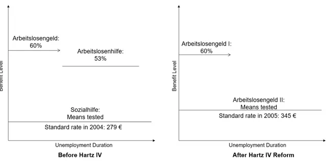
Prior to the Hartz IV reform, the German unemployment benefit system consisted of three lay- ers. ⁷ Upon beginning of a new unemployment spell, workers received short-term unemploy- ment benefits (“Arbeitslosengeld”), which amounted to 60-67% of the previous net earnings ⁸ were paid up to 32 months. After the expiration of short-term benefits, the unemployed received long-term unemployment benefits (“Arbeitslosenhilfe”), which amounted to 53-57% of the prior net earnings and could be awarded until retirement. If unemployed workers did not qualify for these transfers (e.g. because they did not have a sufficiently long employment history), they could apply for means-tested social assistance (“Sozialhilfe”). As part of the reform, the propor- tional long-term unemployment benefits and social assistance were merged to “Arbeitslosengeld II” (ALG II), which is purely means tested based on household income and wealth. The stan- dard rate in 2005 for a single household was 345 Euro (plus a limited reimbursement for rent).

Thus, the system was merged into two pillars, switching to a means-tested system for the long- term unemployed. In addition, as a second component of Hartz IV, the maximum duration of short-term unemployment benefits for older workers, in particular, those above 57, was reduced significantly in 2006. See Figure 2 for an illustration.

6

Our paper is further complementary to a recent literature on the cross-sectional implications of labor selection (see Baydur, 2017, Carrillo-Tudela, Gartner, and Kaas, 2020, and Lochner, Merkl, Stüber, and Gürtzgen, 2021).

7

Hartz IV was part of a sequence of labor market reforms (the Hartz reforms), for details on the Hartz reforms, see Appendix A.

8

The higher rate was awarded to recipients with children.

Figure 2: Illustration of the Hartz IV reform for single households.

As a rule of thumb, the cut of benefits for long-term unemployed was larger for high income and high wealth households. The former faced a large drop because in the new system transfers are no longer proportional to prior earnings and high spousal income may lead to ineligibility. The latter faced a large drop because they may have been ineligible for benefits before running down their wealth.

This institutional setting explains why it is difficult to quantify the decline of the replacement rate due to Hartz IV. Some groups faced a strong reduction of the replacement rate. A single median- income earner faced a drop of 69% according to the OECD tax-benefit calculator (Seeleib-Kaiser, 2016). By contrast, some low-income households (without wealth) saw a slight increase of their replacement rate. It is very difficult to weigh these groups properly because low-skilled workers are overrepresented in the pool of long-term unemployed and their benefits changed the least with the reform.

It is therefore not surprising that one of the key reasons for the diverging results in existing macroeconomic studies are different values for the decline of the replacement rate. Launov and Wälde (2013) use a decline of the replacement rate for long-term unemployed of 7%. Krebs and Scheffel (2013) use a decline of 20% for the replacement rate, while in Krause and Uhlig (2012) the reduction is around 24% for low-skilled workers and around 67% for high-skilled workers.

As a result, unemployment declines by 0.1 percentage points in Launov and Wälde (2013), by 1.4

percentage points in Krebs and Scheffel (2013) and by 2.8 percentage points in Krause and Uhlig

(2012). Given the mentioned difficulties in quantifying the decline of the replacement rate and

the resulting consequences for the effects on unemployment, we directly estimate the partial

effect and the relative size of partial and equilibrium effect. The estimated effects are used as

calibration targets for the model.

3 The Model

Our model economy consists of a unit mass of infinitely lived, risk neutral, atomistic multi- worker firms and infinitely lived, risk neutral workers. ⁹ We use an enhanced version of the Diamond-Mortensen-Pissarides (DMP) model (e.g. Pissarides, 2000, Ch.1) in discrete time. The model is enriched in two dimensions: First, we assume that the hiring process consists of two stages. At the first stage, workers and firms get in contact with one another via a contact function.

In the second stage, firms only select a certain fraction of all contacts because each worker-firm pair is hit by an idiosyncratic training costs shock. The selection rate depends on the aggregate state of the economy and on unemployment benefits. Second, we add a rich unemployment duration structure for unemployed workers with different contact efficiencies and fixed hiring costs. Workers can either be employed or unemployed. Unemployed workers randomly search for jobs on a single labor market. Unemployed workers differ in their unemployment duration.

They are indexed by the letter d , where d ∈ { 0, 1, . . . , 12 } denotes the time left in months that a worker is still eligible for short-term unemployment benefits b ^s , while receiving long-term ben- efits b ^l afterwards. Therefore, a worker who has just lost a job receives the index 12, while a worker indexed by 0 is long-term unemployed.

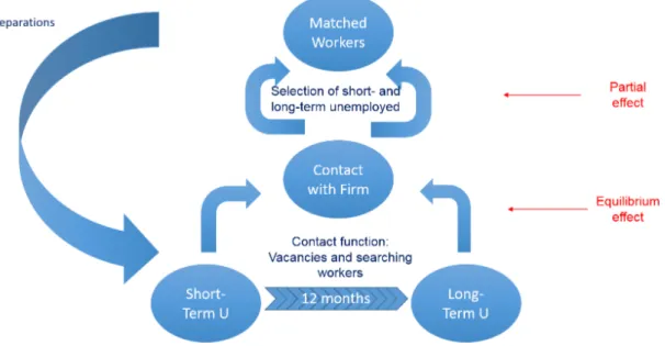
Figure 3: Graphical model description

Figure 3 illustrates the main features of the model. Our model is similar to that in Kohlbrecher, Merkl, and Nordmeier (2016), to the stochastic job matching model (Pissarides, 2000, chapter 6) or many of the endogenous separation models (e.g. Krause and Lubik, 2007). Chugh and Merkl (2016), Lechthaler, Merkl, and Snower (2010), and Sedlá˘cek (2014) are further examples of labor selection models. Except for different unemployment durations, which are essential for the re- form, we do not model further heterogeneities in our theoretical framework (e.g. permanent skill differentials or wealth differentials among unemployed workers). The reason is that the IAB Job

9

For better comparison with establishment-level data, we solve a multi-worker firm’s optimization problem. How-

ever, under constant returns to scale, the results are identical to a one worker-one firm setup.

Vacancy Survey does not provide sufficient guidance on the selection rate in these dimensions.

Thereby, the results across groups would be driven by modeling and parametrization choices instead of being disciplined by the data.

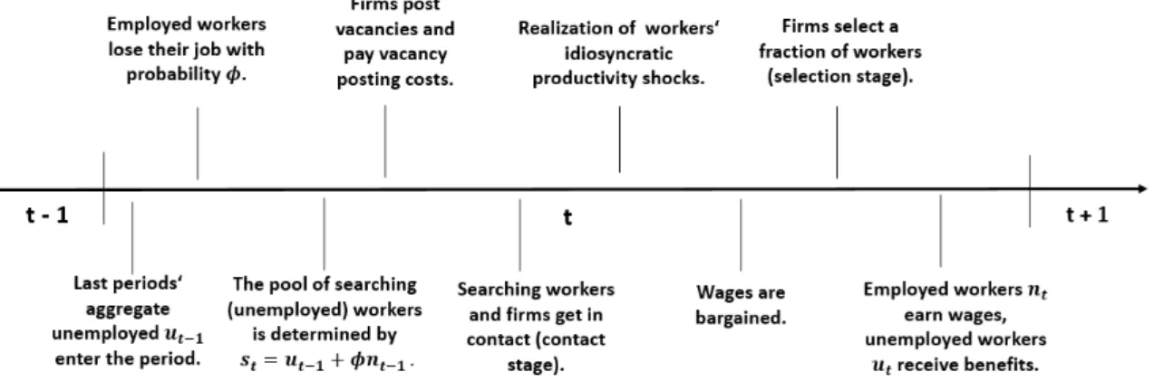
Figure 4: Timeline of the Model

Figure 4 shows the timing of the model. Separated workers can immediately be re-matched.

Therefore, the pool of searching workers, s _t , consists of unemployed workers from the previous period and workers that are separated at the beginning of the period.

3.1 Firms

There is a continuum of atomistic multi-worker firms indexed by i on the unit interval. Firms produce with a constant returns technology with labor as the only input. Employed workers lose their job with constant exogenous probability φ. In order to hire new workers, firms have to use two instruments. First, firms have to post a vacancy to get in contact with a random worker from the unemployment pool. Searching workers and vacancies are connected with a contact function. Second, firms select a certain fraction of those workers they got in contact with. Tech- nically, firms and workers draw a match-specific realization " i t from an idiosyncratic training costs distribution with stable density f (") and cumulative density F (") . Further, we assume a fixed training cost component tc ^d that reflects that the average training required upon reem- ployment depends on the duration of the prior unemployment spell. This is consistent with the idea that human capital may depreciate during unemployment.

Firms are intertemporal profit maximizers. Their revenues consists of aggregate productivity,

a _t , multiplied with firm-specific employment, n _{i t} . Their costs consist of wages for incumbent

workers, w _{i t} ^I , that are retained from the previous period plus wages and recruiting costs for newly

hired workers. The latter consist of linear vacancy posting costs, κ , for each vacancy, v _{i t} , average

wage costs for these new workers, ¯ w _{i t} ^d , and average training costs that contain a stochastic and

a fixed part ( ¯ H _{i t} ^d + tc ^d ). Firms post vacancies in an undirected search market. Once they have

posted a vacancy, they randomly get in contact with an unemployed worker of any of the duration

groups d . The probability for a firm of hiring an unemployed worker indexed by duration d

depends on three factors: the share of unemployed workers indexed by d among all the searching

workers % ^d _t , the contact probability within this duration group q _t ^d (which depends on aggregate market tightness), and the firm’s selection rate, η ^d _{i t} = η " ˜ _{i t} ^d

, which depends on the hiring cutoff

" ˜ ^d _{i t} .

Representative atomistic firms maximize the net present value of profits (discounting with δ ) with respect to employment n _{i t} , vacancies v _{i t} and hiring cutoffs ˜ " _{i t} ^d for all duration groups:

E ₀

¨ _∞ X

t=0

δ ^t ”

a _t n _{i t} − w _{i t} ^I ( 1 − φ) n _{i,t −1} − κ v _{i t} − v _{i t} P ₁₂

d = 0 % ^d _t q _t ^d η ^d _{i t} ( w ¯ _{i t} ^d + H ¯ _{i t} ^d + tc ^d ) —

«

, (3.1)

subject to the evolution of the firm-specific employment stock, and the definitions of selec- tion rates, the average idiosyncratic training costs and entrant wages (both conditional on being hired) for each duration group:

n _{i t} = ( 1 − φ) n _{i,t −1} + v _{i t}

12

X

d = 0

% _t ^d q _t ^d η ^d _{i t} , (3.2)

η ^d _{i t} = Z " ˜

−∞

f (") d " ∀ d , (3.3)

H ¯ _{i t} ^d = R " ˜

−∞ " f (") d "

η ^d _{i t} ∀ d , (3.4)

¯ w _{i t} ^d =

R " ˜

−∞ w (") f (") d "

η ^d _{i t} ∀ d . (3.5)

Maximization of the intertemporal profit function yields the optimal cutoff points and optimal number of vacancies posted by firms:

" ˜ ^d _{i t} = a _t − w ˜ _{i t} ^d − tc ^d + δ(1 − φ) E _t π _{i t} ^I _{+ 1} ∀ d , (3.6) and

κ =

12

X

d=0

% _t ^d q _t ^d η ^d _{i t} π ¯ ^d _{i t} , (3.7) where π ^I _{i t} and π ^d _{i t} denote the firm’s discounted profit at time t for an incumbent worker (indexed by I ) and a newly hired worker in duration group d :

π ^I _{i t} = a _t − w _{i t} ^I + δ( 1 − φ) E _t π ^I _{i t + 1} , (3.8)

π ¯ ^d _{i t} = a _t − w ¯ _{i t} ^d − H ¯ _{i t} ^d − tc ^d + δ( 1 − φ) E _t π ^I _{i t + 1} . (3.9)

Note that all variables with a “tilde” sign are evaluated at the cutoff training costs ˜ " _{i t} ^d , while vari-

ables with a “bar” (such as ¯ H _{i t} ^d ) correspond to the expectation of the respective variable con-

ditional on hiring (i.e. the evaluation of the variable at the conditional mean of idiosyncratic training costs and/or wages). Intuitively, equation (3.6) shows that a firm selects workers in each duration group up to the point where the expected discounted present value of profits for the marginal worker is equal to his training costs. Only contacts with sufficiently low training costs,

" i t ≤ " ˜ ^d _{i t} , will result in a hire, where ˜ " _{i t} ^d is firm i ’s hiring cutoff and η ^d _{i t} = η( " ˜ _{i t} ^d ) is the firm’s selec- tion rate (i.e. the hiring probability for a contact in a specific duration group). Although we call η ^d _{i t} the selection rate, it is important to emphasize that decisions are based on the joint worker- firm surplus of a given contact. Workers will be selected whenever there is a positive joint surplus, i.e. in this case workers are also willing to accept the job.

Equation (3.7) shows that a firm posts vacancies up to the point where the costs, κ , are equal to the expected returns from posting a vacancy. As search is undirected in our model, the firm may get in contact with workers of different duration groups, depending on their share in the unemployment pool % ^d _t and the contact probability. The contact probability for each duration group, q _t ^d , is driven by a Cobb-Douglas, constant returns to scale (CRS) contact function

c _t ^d = µ ^d _t v _t ^γ s _t ^1−γ ∀ d , (3.10) where s _t are the number of searching workers, v _t is the vacancy stock, c _t ^d is the number of con- tacts in period t made with unemployed with duration d , and µ ^d _t is the contact efficiency that depends on the duration of unemployment.

Different contact efficiencies for different duration groups mean that (at a given market tight- ness) some duration groups may have an exogenously lower probability to meet with a firm than others. This is in line with the well-known fact that the job-finding rate is lower for longer- term unemployed than for shorter-term unemployed. As the job-finding rate is the combina- tion of contacts and selection, we calibrate the contact efficiency based on the survey responses whether certain unemployment groups received a job interview or not.

The contact probability for a firm and a worker in a given duration group are therefore:

q _t ^d (θ t ) = µ ^d _t θ t ^γ−1 , (3.11) and

p _t ^d (θ t ) = µ ^d _t θ t ^γ ∀ d , (3.12) with aggregate market tightness defined as

θ t = v _t

s _t . (3.13)

Intuitively, more searching workers generate the usual market externality for other workers and

more searching vacancies for other firms. Note the market externality happens at the level of all

workers.

3.2 Workers

Workers have linear utility over consumption and discount the future with discount factor δ . Once separated from a job, a worker is entitled to 12 months of short-term unemployment ben- efits b ^s and long-term unemployment benefits b _t ^l afterwards, with b ^s > b _t ^l .

The value of unemployment therefore depends on the remaining months a worker is eligible for short-term unemployment benefits. For a short-term unemployed (i.e. d ∈ {1, . . . , 12}) the value of unemployment is given by:

U _t ^d = b ^s + δ E _t

p _t ^d−1 _{+ 1} η ^d−1 _{t + 1} V ¯ _t ^d ₊ ⁻¹ ₁ + ( 1 − p _t ^d−1 _{+ 1} η ^d−1 _{t + 1} ) U _t ^d−1 _{+ 1}

. (3.14)

In the current period, the short-term unemployed receives benefits b ^s . In the next period, she either finds a job or remains unemployed. In the latter case the time left in short-term unem- ployment d is reduced by a month. The probability of finding employment in the next period will depend on the next period’s contact probability and selection rate, which both depend on unemployment duration at that point.

After 12 months of unemployment the worker receives the lower long-term unemployment ben- efits b _t ^l indefinitely or until she finds a job:

U _t ⁰ = b _t ^l + δ E _t

p _t ⁰ _{+ 1} η ⁰ _{t + 1} V ¯ _t ⁰ _{+ 1} + ( 1 − p _t ⁰ _{+ 1} η ⁰ _{t + 1} ) U _t ⁰ _{+ 1}

. (3.15)

The value of work for an entrant depends through the wage on the remaining months she is eligible for short-term benefits and on the realization of the idiosyncratic training cost:

V _t ^d (" t ) = w _t ^d (" t ) + δ E _t

( 1 − φ) V _t ^I _{+ 1} + φ U _t ^I _{+ 1}

∀ d . (3.16)

Following our previous notation, ¯ V _t ^d corresponds to the evaluation of V _t ^d (" t ) at the conditional expectation of " t . We allow for the possibility of immediate rehiring. The resulting value of work for an incumbent worker I is:

V _t ^I = w _t ^I + δ E _t

( 1 − φ) V _t ^I ₊₁ + φ p _t ¹² η ¹² _t V ¯ _t ¹² + ( 1 − p _t ¹² η ¹² _t ) U _t ¹²

. (3.17)

3.3 Wages

In the main part of the paper, we assume individual Nash bargaining for both new and existing matches. Workers and firms bargain over the joint surplus of a match, where workers’ bargaining power is α and firms’ bargaining power is ( 1 − α) . The Nash bargained wages therefore solve the following problems:

w _t ^d (" t ) ∈ arg max V _t ^d (" t ) − U _t ^d _α

π ^d _t (" t ) _1−α

∀ d (3.18)

for newly hired workers with prior duration index d and w _t ^I ∈ arg max V _t ^I − U _t ^I _α

π ^I _{t 1−α}

(3.19)

for an incumbent worker.

Maximizing the Nash product yields the following wage equations for incumbents w _t ^I =α

a _t + δ p _t ¹² η ¹² _t E _t π ^I _{t +1}

(3.20) + ( 1 − α)

− p _t ¹² η ¹² _t E _t

(δ V _t ^I ₊₁ − V ¯ _t ¹² )

− ( 1 − p _t ¹² η ¹² _t ) E _t

(δ U _t ^I ₊₁ − U _t ¹² ) , and different duration groups of entries:

w _t ^d (" t ) =α

a _t − " t − tc ^d + δ E _t

p _t ^d−1 _{+ 1} η ^d−1 _{t + 1} π ^I _{t + 1}

(3.21) + (1 − α)

b ^S − δE t p _t ^d−1 _{+ 1} η ^d−1 _{t + 1} (V _t ^I _{+ 1} − V ¯ _t ^d ₊ ⁻¹ ₁ ) − δE t

(1 − p _t ^d−1 _{+ 1} η ^d−1 _{t + 1} )(U _t ^I _{+ 1} − U _t ^d−1 _{+ 1} )

∀ d ∈ { 1, . . . , 12 } , w _t ⁰ (" t ) =α

a _t − " t − tc ⁰ + δ E _t

p _t ⁰ _{+ 1} η ⁰ _{t + 1} π ^I _{t + 1}

(3.22) + ( 1 − α)

b _t ^L − δ E _t p _t ⁰ ₊₁ η ⁰ _{t +1} ( V _t ^I ₊₁ − V ¯ _t ⁰ ₊₁ ) − δ E _t

( 1 − p _t ⁰ ₊₁ η ⁰ _{t +1} )( U _t ^I ₊₁ − U _t ⁰ ₊₁ ) . Note that these equations would collapse to the standard Nash bargaining solution if we just had one duration group. Several things are worth emphasizing: The benefits for long-term un- employed directly affect the wage for long-term unemployed, as they are part of their outside option. They also affect the wage of short-term unemployed. However, this happens in an indi- rect way through the expected value of long-term unemployment E _t U _t+1 ⁰ . Obviously, the outside option and thereby the wage will be affected more by changes of b ^L , the closer workers are to long-term unemployment.

The individually bargained wage depends on the individual idiosyncratic training cost realiza- tion. ¹⁰ In D.3 we show results for the case when wages are bargained collectively.

3.4 Unemployment Dynamics

As the total labor force is normalized to one, the total number of unemployment (and also the unemployment rate) in period t after matching has taken place is the sum over all unemploy- ment states (d ∈ { 0, ..., 12 } ):

u _t =

12

X

d = 0

u _t ^d . (3.23)

Unemployment in period t is thus given by

u _t = 1 − n _t . (3.24)

The number of unemployed with 12 remaining months of short-term benefits is given by the workers that have been separated at the end of last period and were not immediately rehired:

u ¹² _t = φ(1 − p _t ¹² η ¹² _t ) n _{t −1} . (3.25)

10

The wage for entrants is smaller than the wage for incumbents in our bargaining set-up due to training costs, and

because longer-term unemployment is associated with higher fixed training costs in our calibration. However, the

net present value of the match for workers and firms at the time of hiring is equivalent to a wage contract where

the training costs in the wage are spread over the entire employment spell. Results are available on request.

The law of motion for unemployment with remaining eligibility of short-term unemployment benefits d ∈ {1, . . . , 11} is:

u ^d _t = ( 1 − p _t ^d η ^d _t ) u ^d _{t −1} ^{+ 1} , (3.26) and the pool of long-term unemployed consists of the unemployed whose short-term benefit eligibility has just expired as well as previous period’s long-term unemployed that have not been matched:

u _t ⁰ = (1 − p _t ⁰ η ⁰ _t )(u _t ¹ ₋₁ + u _t ⁰ ₋₁ ). (3.27) We can now define the number of searching workers at the beginning of period t (before match- ing has taken place):

s _t = φ n _{t −1} + u _{t −1} . (3.28)

The share of searching workers with remaining short-term unemployment eligibility of d months among all searchers is therefore:

% ¹² _t = φ n _{t −1}

s _t , (3.29)

for newly separated workers,

% ^d _t = u ^d _{t −1} ^{+ 1}

s _t , (3.30)

for d ∈ { 1, . . . , 11 } and

% _t ⁰ = u ¹ _{t −1} + u ⁰ _t−1

s _t (3.31)

for long-term unemployed.

3.5 Labor Market Equilibrium

Given initial values for all states of unemployment u ^d _t−1 with d ∈ {0, ..., 12} and employment n _{t −1} as well as processes for productivity, long-term unemployment benefits, and the spell- dependent contact efficiency

a _t , b _t ^l , µ ^d _t ^+∞ _{t = 0} , the labor market equilibrium is a sequence of allo- cations

n _t , u _t , s _t , v _t , θ t , u _t ^d , % ^d _t , p _t ^d , q _t ^d , ˜ " _t ^d , η ^d _t , ¯ H _t ^d , π ^I _t , ¯ π ^d _t , V _t ^I , ¯ V _t ^d , ˜ V _t ^d ,U _t ^I ,U _t ^d , w _t ^I , ¯ w _t ^d , ˜ w _t ^{d +∞} _{t = 0} for all durations d ∈ { 0, ..., 12 } that satisfy the following equations: the definition of employment (3.24), unemployment (3.23) and searching workers (3.28), market tightness (3.13), unemploy- ment (3.25) - (3.27), the shares of searching workers (3.29) - (3.31), the contact rates for workers (3.12) and firms (3.11), the free-entry condition for vacancies (3.7), the hiring cutoffs (3.6), selec- tion rates (3.3), conditional expectation of idiosyncratic hiring costs (3.4) and wages (3.5) ¹¹ , the definition of profits for entrants (3.9) and incumbents (3.8), the value of a job for entrants (3.16) and incumbents (3.17), the value of unemployment (3.14), and (3.15), and wages (3.20), (3.21) and (3.22).

11

In equilibrium, all atomistic firms behave symmetrically. Therefore, we can drop the firm indices i in the previous

five equations.

4 Empirical Results

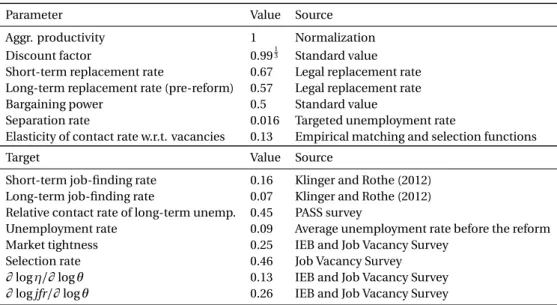
While there is agreement that the Hartz IV reform reduced the generosity of long-term unem- ployment benefits, there is no consensus on the exact quantitative decline of the replacement rate (see Section 2 for details). This poses a challenge for any model-based macroeconomic evaluation. In order to circumvent this problem, we propose a new strategy based on the IAB Job Vacancy Survey.

Our empirical strategy is based on measuring three objects: (i) the permanent shift of selection in response to the reform, (ii) the elasticity of the selection rate w.r.t. market tightness and (iii) the elasticity of the job-finding rate w.r.t. market tightness. The first object pins down the partial effect in our framework. The second and third objects determine the relative size of the partial and equilibrium effects. We use the estimated results as calibration targets for our quantitative exercise (see Section 5).

4.1 Measuring Selection

In our model, a multi-worker firm can adjust the workforce along two margins. First, it can change the number of posted vacancies. Depending on aggregate market tightness, this deter- mines the number of applicants (vacancies multiplied with q _t ) that get in contact with the firm.

Second, the firm selects a certain fraction of these applicants, η t . In our model, the selection rate corresponds to the number of hires divided by the number of contacts ( ^η _v

^v

^q

t

q

).

Why does the selection rate increase when unemployment benefits decline? Lower unemploy- ment benefits increase the joint surplus of a match. Therefore, a larger fraction of workers, η t , is selected upon contact. Assume for illustration purposes that a multi-worker firm chose 33%

of contacts before the reform and 50% of contacts after the reform. In this case, it had on aver- age three contacts per hire before the reform and two contacts per hire after the reform. Thus, our model predicts that the selection rate rises and the number of contacts per hire decrease in response to the reform (see Appendix D.1 for an illustration).

We use the IAB Job Vacancy Survey to proxy the selection rate. The IAB Job Vacancy Survey is an annual representative survey of up to 14,000 German establishments (for more information on the dataset, see Appendix B.1). Ideally, we would measure the selection rate as the ratio of all hires over all applicants ( ^η _v

^v

^q

t

q

). However, in the IAB Job Vacancy Survey, we only have information on firms’ recruiting situation for the most recent hire. Firms are asked about the number of suitable applicants, ¹² which we use as a proxy for the selection rate by taking the inverse. Hence, from the perspective of an applicant, this represents his or her probability of being selected (upon contact) by the firm. Both our choice of “suitable applicants” and the focus on the most recent hire require some more discussion.

We believe that the notion of “suitable applicants” is well in line with our model. ¹³ First, as firms consider these applicants as suitable, they must have screened them in some way (e.g. by check-

12

While this information is available for a long-time period, the total number of applicants is only available from 2005 onwards and therefore not suitable for our question at hand.

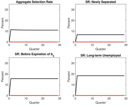
13

To provide intuition, we illustrate the model reaction of the total number of contacts and contacts per hire in re-

sponse to a reduction of the replacement rate for long-term unemployed in Appendix D.1 for our baseline calibra-

tion.

ing the CV or by inviting them to an interview). Thus, through the lens of our model, the contact function established a contact between firms and applicants. Second, when firms answer how many suitable applicants they had for a given position, we expect that these applicants were suit- able in terms of observable characteristics (e.g. skills or experience.) This is also in line with our model where we abstract from observable characteristics. Ex-ante homogeneous applicants are ex post heterogeneous in terms of an idiosyncratic shock realization in our model. Although ap- plicants may appear suitable in terms of their qualifications or their CV, a more detailed screen- ing may uncover that the candidates have unfavorable characteristics (i.e. high training costs in terms of our model). ¹⁴

Given that we only have information for the most recent hire (and not all hires), it is important to ensure representativity. Several comments are in order: First, when employers made several simultaneous hirings, the survey asks about the hired individual whose surname comes first in alphabetical order (i.e. randomness is imposed). Second, while a given vacancy may not be rep- resentative at a particular firm (e.g. if the firm hires one high-skilled and one low-skilled worker, the firm reports on the most recent hire), we use representative survey weights to ensure rep- resentativity at higher aggregation levels (e.g., state, industry, national). The last step allows us to obtain a panel dimension at the industry and state level. As the IAB Job Vacancy Survey is a repeated cross section, we can only perform panel regressions at an aggregated level in any case.

Using our measure of the selection rate, we construct annual time series on the national (West Germany as a baseline and entire Germany as robustness ¹⁵ ), state and industry level from 1992 to 2019.

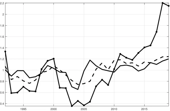
Figure 5 shows the time series of the job-finding rate (defined as matches over unemployment), selection rate and market tightness (defined as vacancies over unemployment) from 1992 to 2019 (for details on the data, see Appendix B). We normalized all three time series to a mean of one to improve the visibility of relative movements (i.e. we divided each time series by its sample mean).

As predicted by theory, both the job-finding rate and the selection rate move procyclically with market tightness, although the latter shows much stronger fluctuations (see Appendix C for a discussion).

4.2 Estimation Strategy

As the aggregate contact and selection rate are roughly multiplicative in our model (jfr _t ≈ p _t η t ), ¹⁶ we can express the job-finding rate, ˆ jfr _t , as the sum of the contact rate, ˆ p _t , and the se- lection rate, ˆ η t , in terms of log-deviations (denoted with hats):

14

Under the new and stricter benefit regime workers are required to document search effort, e.g. in forms of written applications. Two scenarios are possible: Either, these forced applications are not meaningful and do not make it into the pool of suitable applicants. In this case the selection rate would be unaffected. Alternatively, the number of suitable applicants increases and lowers the measured selection rate, which would bias our estimate for the selection rate downward, i.e. we would obtain a lower bound.

15

We restrict the baseline analysis to West Germany for two reasons. First, the conditions in East Germany were driven by the transformation to a market economy in the 1990s. Labor market turnover rates in East Germany have converged to those of West Germany only by 2008 (see Fuchs, Jost, Kaufmann, Ludewig, and Weyh, 2018).

Second, the number of establishments in the sample is very small in the early 1990s.

16

Note that this connection holds with equality for each duration group jfr

= p

η

. In aggregate, it only holds with

equality on impact when the shares of unemployed workers in different duration groups are equal to the steady

state shares. During the adjustment dynamics, composition effects start playing a role.

Figure 5: German labor market dynamics, 1992-2019.

1995 2000 2005 2010 2015

0.4 0.6 0.8 1 1.2 1.4 1.6 1.8 2 2.2

Job-Finding Rate (Normalized to 1) Selection Rate (Normalized to 1) Market Tightness (Normalized to 1)

Note: For visibility, we normalized all three time series to mean one. The job-finding rate (matches over unemploy- ment) and market tightness (vacancies over unemployment) are constructed with the corrected unemployment series (as described in Appendix E.3). For details on the data sources, see Table B.1 in Appendix B.

jfr ˆ _t ≈ p ˆ _t + η ˆ t . (4.1)

We refer to the response of the selection rate to a benefit change as the partial effect and the response of the contact rate as equilibrium effect.

In order to quantify the macroeconomic reaction of the job-finding rate with respect to changes in long-term unemployment benefits, we proceed in two steps. First, we estimate the reaction of the selection rate with respect to changes of benefits ( ∂ η ˆ t /∂ b ˆ _t ), i.e. the partial effect. Sec- ond, we use the connection that the overall macroeconomic effect can be disentangled into the equilibrium effect ( ∂ p ˆ _t /∂ b ˆ _t ) and the partial effect:

∂ jfr ˆ _t

∂ b ˆ _t ≈ ∂ p ˆ _t

∂ b ˆ _t + ∂ η ˆ t

∂ b ˆ _t . (4.2)

Estimating the effects of benefits on labor selection has two advantages compared to estimat- ing the effects of benefits on the job-finding rate. First, selection happens after contacts were established. Thus, there is no direct effect of improved matching efficiency on selection. This is important because of the reform the Federal Employment Agency in 2003 (Hartz III), which according to Launov and Wälde (2016) improved matching efficiency. ¹⁷ Second, in contrast to

17

In our setting, this would be equivalent to an increase in the contact efficiency. We analyze the effect of an increase

in the contact efficiency in Appendix D.4 and show that this would bias our results downwards.

the time series for the job-finding rate (which is calculated as matches over unemployed), the se- lection rate does not suffer from a severe statistical break in 2005 (see Appendix E for a detailed discussion). Against this background, we use a simple shift dummy (which is one from 2005 on- wards) to determine the effects of the Hartz IV reform on selection. In addition, we control for business cycle and composition effects.

In a second step, we determine the relative importance of the equilibrium effect. For this pur- pose, we use the following relationship from our model:

∂ p ˆ _t /∂ b ˆ _t

∂ η ˆ t /∂ b ˆ _t ≈ ∂ p ˆ _t /∂ θ ˆ t

∂ η ˆ t /∂ θ ˆ t

. (4.3)

We can show numerically that this feature holds approximately in our full quantitative model. ¹⁸ Note that selection, job finding and market tightness positively comove with aggregate produc- tivity in our model. Up to a first-order Taylor approximation, there is a linear comovement be- tween productivity and tightness.

The relative importance of the partial and the equilibrium effect are the same for a labor market reform and over the business cycle. Intuitively, both an increase of productivity and a reduction of unemployment benefits increase the joint surplus of a match. Thus, they have equivalent effects on the contact and selection margin. Empirically, market tightness is a better indicator for the labor market stance than productivity. Therefore, we use this measure to determine the relative importance of the partial and equilibrium effects.

The contact rate is not observable in the data. But the elasticity of the contact rate and selec- tion rate approximately add up to the elasticity of the job-finding rate with respect to market tightness:

∂ jfr ˆ _t

∂ θ ˆ t

≈ ∂ p ˆ _t

∂ θ ˆ t

+ ∂ η ˆ t

∂ θ ˆ t

. (4.4)

Therefore, we can estimate the comovement of the job-finding rate and the selection rate with market tightness. We impose these elasticities in our calibrated model and thereby discipline the relative size of the partial and equilibrium effects by their business cycle movements.

4.3 Baseline Results

To estimate the partial effect, the logarithm of the selection rate is regressed on a shift dummy that takes the value of one from 2005 onward (D _t ^{Hartz IV} ). The shift dummy measures the perma- nent differences of the selection rate before and after Hartz IV. To disentangle the partial effect from the equilibrium effects, we control for business cycle fluctuations (either in terms of value added or market tightness):

log η t = β 0 + β 1 D _t ^{Hartz IV} + β 2 X _t + ν t , (4.5)

where X _t denotes a business cycle control (such as value added growth or market tightness). Due to data availability, we perform the baseline estimation on an annual basis for the sample range

18

For an analytical illustration in the context of a simplified model see Appendix D.2.

1992 to 2019 for West Germany.

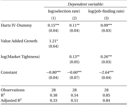
Columns 1 and 2 in Table 1 show that conditional on value added or market tightness fluctuations the aggregate selection rate has increased by 15% or 11% respectively after the Hartz IV reform.

The estimated coefficients are statistically significant at the 5% level. ¹⁹ We take the more con- servative second value as calibration target. Although our baseline result is based on very simple specification, we show in the next subsection that it is robust in various dimensions (e.g. con- trolling for composition, testing for the time structure, disaggregating to the regional or industry level).

Table 1: Regression Results for West Germany, 1992-2019.

Dependent variable:

log(selection rate) log(job-finding rate)

(1) (2) (3)

Hartz IV-Dummy 0.15

0.11

0.09

(0.04) (0.04) (0.03)

Value Added Growth 1.21

(0.64)

log(Market Tightness) 0.13

0.26

(0.05) (0.03)

Constant − 0.80

− 0.60

− 2.64

(0.04) (0.07) (0.04)

Observations 28 28 28

R

0.38 0.54 0.85

Adjusted R

0.33 0.51 0.84

Note: Estimation by OLS with robust standard errors;

p<0.1;

p<0.05;

p<0.01. For details on the data sources, see Table B.1 in Appendix B.

To determine the relative importance of partial and equilibrium effects, we estimate the comove- ment of the job-finding rate and the selection rate with market tightness. ²⁰ Column 2 in Table 1 shows that the estimated elasticity for the selection rate is 0.13. We perform the same regression with the logarithm of the job-finding rate as dependent variable. Column 3 in Table 1 shows an estimated elasticity of 0.26 (which is well in line with existing matching function estimations ²¹ ).

By targeting both estimated elasticities in a dynamic business cycle simulation of our model, we can uniquely pin down the contact elasticity.

19

We use heteroskedasticity-consistent estimators, with a small sample correction proposed by MacKinnon and White (1985)

20

Although we also estimate a shift dummy for the job-finding rate, we do not interpret it (due to the statistical break).

The key purpose of this estimation is the estimation of the elasticity of the job-finding rate with respect to market tightness for determining the size of the equilibrium effect.

21

See e.g. Hertweck and Sigrist (2013) (based on data from the German Socio-Economic Panel) and Kohlbrecher et al.

(2016) (based on detailed administrative data).

4.4 Robustness Checks and Discussion

The estimated partial effects are robust in various dimensions:

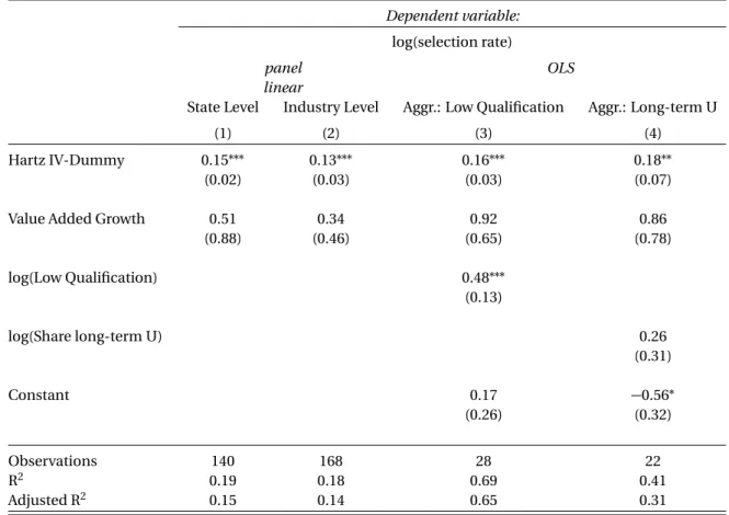
In columns 1 and 2 of Table 2, we show that the results are very similar if we disaggregate by state and industry level and use a panel fixed-effects estimator. Our estimation of the shift dummy may be misinterpreted if the selection rate moves due to composition over time (e.g. as unem- ployed with different skills or durations may have a different selection rate). Our results are ro- bust if we control for the share of vacancies for low-qualification jobs and the share of long-term unemployed in the pool of unemployment (see columns 3 and 4 in Table 2). Appendix E shows further robustness checks with additional controls for the pool of applicants and unemployment along the gender and age dimension (see Table E.2). In addition, controlling for market tightness instead or in addition to value added growth (see Table E.3) does not change the estimated coef- ficient on the Hartz IV-dummy by much.

Table 2: Robustness

Dependent variable:

log(selection rate)

panel OLS

linear

State Level Industry Level Aggr.: Low Qualification Aggr.: Long-term U

(1) (2) (3) (4)

Hartz IV-Dummy 0.15

0.13

0.16

0.18

(0.02) (0.03) (0.03) (0.07)

Value Added Growth 0.51 0.34 0.92 0.86

(0.88) (0.46) (0.65) (0.78)

log(Low Qualification) 0.48

(0.13)

log(Share long-term U) 0.26

(0.31)

Constant 0.17 − 0.56

(0.26) (0.32)

Observations 140 168 28 22

R

0.19 0.18 0.69 0.41

Adjusted R

0.15 0.14 0.65 0.31

Note: Aggregate estimation by OLS with robust standard errors; Panel estimation with fixed effects (state and industry fixed effects respectively) and robust standard errors clustered at group level. Due to data availability, the regression for long-term unemployed covers the shorter time span 1998 - 2019.

p<0.1;

∗∗

p<0.05;

p<0.01. For details on the data sources, see Table B.1 in Appendix B.

Figure F.1 in F shows that the increase of the selection rate between 2004 and 2005 was largest for workers in the middle of the skill distribution. ²² This is in line with our expectations. Compared

22

The question on skills is only available from 2004 onwards. Therefore, we can only provide anecdotal evidence for

to workers in the middle of the skill distribution, low-skilled workers faced a moderate decline of the replacement rate due to the Hartz IV reform (see Section 2), while high-skilled workers usually face short unemployment spells and therefore a lower risk of becoming long-term un- employed. Thus, medium-skilled workers were hit hardest by the Hartz IV reform and thereby reacted most in terms of the selection rate. ²³

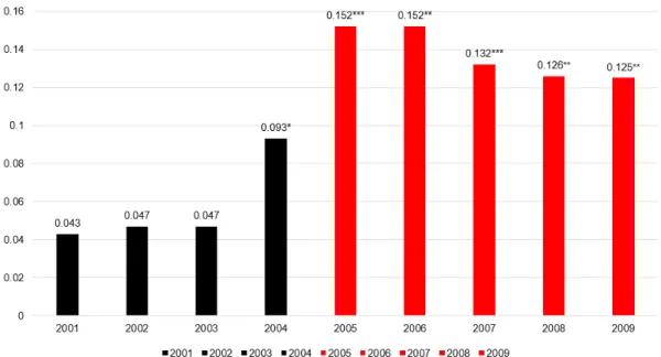
In order to illustrate that our Hartz IV-dummy effect is no coincidence, we perform several re- gressions with placebo shift-dummies in the years before and after the reform. Figure 6 clearly supports our view that the jump of the selection rate took place from 2005 onwards, the time when the first step of the Hartz IV reform was implemented. The shift dummy starts being sta- tistically different from zero at the 5 percent level from 2005 onwards. This is completely in line with our theoretical framework, which predicts that the selection rate increases on a permanent basis once the Hartz IV labor market reform was implemented and remains on a higher level from then onwards. Thus, the shift of the selection rate cannot be attributed to long-run trends such as the wage moderation that started in the early 2000s.

Figure 6: Alternative shift-dummies starting in each respective year (controlling for value added growth).

Note: The red bars denote significant dummy estimates at the 1 percent (***) and 5 percent (**) significance level.

Although we cannot establish a causal relationship between Hartz IV and the partial effect on the selection rate in a microeconometric sense, our approach has two virtues: (i) we create (semi-) aggregated time series that correspond directly to the partial effect in our model, (ii) we show that the selection rate has shifted upwards in an economically and statistically significant way from 2005 onwards. We believe that reverse causality is not an issue in our regressions because the Hartz IV reform was an exogenous event that was certainly not affected by the selection rate. The

the upward shift between 2004 and 2005.

23

While it would be desirable to study the cross-sectional response of the selection rate in more detail, we are limited

by information provided in the data. Information on skills (for the selection rate) is for example not available for a

longer time series.