IHS Economics Series Working Paper 141
October 2003
Multiple Objective Step Function Maximization with Genetic Algorithms and Simulated Annealing
Günther Grohall
Jürgen Jung
Impressum Author(s):
Günther Grohall, Jürgen Jung Title:
Multiple Objective Step Function Maximization with Genetic Algorithms and Simulated Annealing
ISSN: Unspecified
2003 Institut für Höhere Studien - Institute for Advanced Studies (IHS) Josefstädter Straße 39, A-1080 Wien
E-Mail: o ce@ihs.ac.atffi Web: ww w .ihs.ac. a t
All IHS Working Papers are available online: http://irihs. ihs. ac.at/view/ihs_series/
This paper is available for download without charge at:
https://irihs.ihs.ac.at/id/eprint/1518/
141 Reihe Ökonomie Economics Series
Multiple Objective Step Function Maximization with Genetic Algorithms and Simulated Annealing
Guenther Grohall, Juergen Jung
141 Reihe Ökonomie Economics Series
Multiple Objective Step Function Maximization with Genetic Algorithms and Simulated Annealing
Guenther Grohall, Juergen Jung October 2003
Institut für Höhere Studien (IHS), Wien
Institute for Advanced Studies, Vienna
Contact:
Guenther Grohall
Department of Economics and Finance Institute for Advanced Studies Stumpergasse 56
1060 Vienna, Austria : +43/1/599 91-246 email: grohall@ihs.ac.at Juergen Jung
Indiana University 3209 E 10th St Apt H16 Bloomington, IN 47408, USA email: juejung@indiana.edu
Founded in 1963 by two prominent Austrians living in exile – the sociologist Paul F. Lazarsfeld and the economist Oskar Morgenstern – with the financial support from the Ford Foundation, the Austrian Federal Ministry of Education and the City of Vienna, the Institute for Advanced Studies (IHS) is the first institution for postgraduate education and research in economics and the social sciences in Austria.
The Economics Series presents research done at the Department of Economics and Finance and aims to share “work in progress” in a timely way before formal publication. As usual, authors bear full responsibility for the content of their contributions.
Das Institut für Höhere Studien (IHS) wurde im Jahr 1963 von zwei prominenten Exilösterreichern – dem Soziologen Paul F. Lazarsfeld und dem Ökonomen Oskar Morgenstern – mit Hilfe der Ford- Stiftung, des Österreichischen Bundesministeriums für Unterricht und der Stadt Wien gegründet und ist somit die erste nachuniversitäre Lehr- und Forschungsstätte für die Sozial- und Wirtschafts- wissenschaften in Österreich. Die Reihe Ökonomie bietet Einblick in die Forschungsarbeit der Abteilung für Ökonomie und Finanzwirtschaft und verfolgt das Ziel, abteilungsinterne Diskussionsbeiträge einer breiteren fachinternen Öffentlichkeit zugänglich zu machen. Die inhaltliche Verantwortung für die veröffentlichten Beiträge liegt bei den Autoren und Autorinnen.
Abstract
We develop a hybrid algorithm using Genetic Algorithms (GA) and Simulated Annealing (SA) to solve multi-objective step function maximization problems. We then apply the algorithm to a specific economic problem which is taken out of the corporate governance literature.
Keywords
Numerical computation, genetic algorithms, simulated annealing
JEL Classification
G32, G34
Comments
Contents
1 Introduction 1
2 Why Standard Optimization Routines Fail 2 3 The Hybrid Approach 5
3.1 The Genetic Algorithm (GA)... 5
3.2 Simulated Annealing (SA)... 6
3.3 Construction of the GASA-Algorithm ... 7
4 Applying the Algorithm 8
4.1 A Motivating Example ... 94.2 The Theoretical Foundations ... 10
4.3 Data Description ... 12
4.4 The FabFive Results... 13
4.4.1 Dispersed Shareholders Treated as One Single Voter ... 13
4.4.2 Dispersed Shareholders Treated as Single Voters ... 14
4.5 The Network Results ... 16
4.5.1 Dispersed Shareholders Treated as One Block... 16
4.5.2 Dispersed Shareholders Treated as Single Voters ... 18
5 Conclusion 19
References 20
Figures 21
1 Introduction
Genetic Algorithms (GA) and Simulated Annealing (SA) are powerful stochastic global search and optimization methods. They are particularly powerful when applied to problems for which little prior information about the general topology is available. Both methods converge asymptotically probabilistically to a global optimum.
Genetic Algorithms thereby mimic an evolutionary biological process. Gener- ations of solutions are evaluated according to a fitness value and only those can- didates with high fitness values are used to create further solutions via crossover and mutation procedures.
Simulated Annealing simulates the behavior of a system of particles which is gradually cooling down until a strong crystalline structure is reached. In terms of computational simulation, a global minimum would correspond to such a “cold”
(steady) state. Both methods are valid and efficient methods in numeric program- ming and have been employed in various fields due to their strong convergence properties.
1Step function maximization is a challenge for any computer package provid- ing numeric optimization tools. The inherent discontinuities and computational restrictions in approximating stepwise functions cause many standard packages to either break off in its calculations, to hit time limits, to simply miscalculate the solution or to get stuck in local optima.
This paper demonstrates how traditional numerical methods fail on multi- objective step optimization problems and how such problems can be overcome by a hybrid-algorithm which combines elements of Genetic Algorithms and Simu- lated Annealing. We develop a general procedure which is open enough such that it can easily be extended to solve a variety of specific step function problems. For the sake of fast implementation and the possibility to use many pre-programmed functions, Matlab is the chosen platform.
Finally, we use a model of ownership and control
2with large numbers of possible coalitions to examine the effectiveness of the proposed algorithm. In addition, we use data on German corporations to further test the algorithm in an applied setting and solve the model numerically.
In section 2 we introduce the basic setup of our step function maximization problem and problems we encountered using traditional maximization techniques.
Section 3 introduces Genetic Algorithms (GA) and Simulated Annealing (SA) and the implementation of the combined GASA-algorithm. Section 4 describes a complex model of ownership and control structures that seems to be a suitable application for the algorithm. The last section concludes our observations.
1(Wu and Wang, 1998) give an introduction of how Simulated Annealing can be employed to calculate economic equilibria.
2Developped by (Ritzberger and Shorish, 2002).
2 Why Standard Optimization Routines Fail
We start by introducing the general formulation of a multiple-objective step func- tion maximization problem:
max { τ
1, τ
2. . . τ
m} (1)
s.t.
F
τ(Ξ + CΣ) = C and eC = e,
where τ is a vector of positive integers, C is an integer matrix, Ξ and Σ are real numbered matrices, F
τis a nonlinear function, and e is a summation vector of appropriate size which sums up each column of C. Maximizing vector τ means maximizing a weighted indicator which “summarizes” all entries in τ (e.g. the norm or any other criterion). We have found a maximum if it is not possible anymore to increase an entry in τ without violating a constraint.
Next we define a real numbered n × m input matrix X = [x
1· · · x
m] ∈ R
+n×mand define function F
τ(X) : R
n×m+→ Z
+n×mF
τ(X) =
f
τ(1)(x
1) · · · f
τ(m)(x
m)
(2) such that F is composed of step functions:
3f
t(x) = (f
1t. . . f
nt)
0: R
n+→ Z
+n(3) applied on each single column vector in X. Function F also depends on a vector τ of integers, τ = (τ
1, τ
2. . . τ
m) ∈ Z
+m. This vector puts additional structure on function F .
Next we define a control matrix C
n×mwith entries c
ij∈ C = { 0, 1 } as integer switching variables. The additional restriction eC = e, makes sure that the sum of each column in C is 1, hence only one entry per matrix column is equal to one, all other entries are zero. In addition, we impose that C enters the function F in the (non-integer) form Ξ + CΣ, where Ξ and Σ are arbitrary real value matrices defined as Ξ ∈ R
n×m+and Σ ∈ R
+m×m. The output of function F , will be of the same integer form as C.
In (1) the constraint is formulated as a fixed-point search. Function F
τmaps the actual set of control coefficients into a new such set. In other words, an equilibrium is a matrix C which is reproduced by the following iteration, given a maximum integer vector τ . Since our constraint function is a fixed-point problem we can also represent the entire integer system in hierarchical form as a double
3We are not restricted to the integer set Z+n. We could also map f into Rn+ and partition the range off into any subset ofRn+, as long as the step character off is maintained.
2
optimization problem:
max { τ
1, τ
2. . . τ
m} s.t.
min
C[F
τ(Ξ + CΣ) − C]
s.t.
eC = e
This formulation allows us, to use different algorithms for the master problem (objective function) and the slave problem (first constraint).
Since the optimization-routines provided by Matlab work best on continuous functions, we replace one discrete part of the optimization problem, the function f
twith a continuous approximation of the discrete step function defined as:
4g
t(x, ) = (g
1t. . . g
nt)
0: R
n+→ R
n+(4) Parameter determines how “good” function g
tapproximates the discrete step- function f
t. Computation time increases sharply with small values, due to combinatorics in the approximation function g
t. Function F then becomes func- tion G
τ(X) : R
n×m+→ R
n×m+which is composed as:
G
τ(X) =
g
τ(1)(x
1) · · · g
τ(m)(x
m)
As a first approach we develop small test cases for which it is relatively easy to cal- culate all solution manually. We then check whether pre-programmed computer routines find the same correct results within feasible time. The step function system for these test cases are not larger than C
3×5and thus τ = [τ(1) · · · τ(5)].
In a first attempt, we use the internal Matlab function fmincon, which pro- vides various options to minimize continuous functions given a number of con- straints. In order to use fmincon we have to reinterpret (1) as a minimization problem:
min( − τ) s.t. [G
τ(Ξ + CΣ) − C]
.2= [0] and eC = e, (5) where
.2squares a matrix pointwise instead of multiplying the matrix with itself and [0] is a zero-matrix of size m × n. The second constraint can be calculated easily, but for the first, we have to find a suitable set of control coefficients C.
This fixed-point problem is itself a minimization problem and we can therefore rewrite (5) as a double minimization with one constraint:
min( − τ) s.t.
n
min
C[G
τ(Ξ + CΣ) − C]
.2s.t. eC = e o
(6)
4Compare appendix in (Ritzberger and Shorish, 2002).
As long as the result of minimizing G
τleads to a zero-matrix and the sum of each column equals 1, the vector − τ has to be minimized. This minimization problem is implemented and applied on the small test cases.
The results are poor, suggesting that this method will not work for larger data-sets. The most difficult problem is that convergence depends heavily on the starting values of C. A good combination of C and leads to convergence towards control coefficients c
ij∈ C with values ranging between 0.6 and 0.9 where a 1 would be the correct solution. We get values between 0.1 and 0.2 where entries should be zero instead. This is not necessarily a problem, since after rounding these values we could use them recursively as input in the constraint of (1). If the resulting C is the same as the one used as input, a fixed-point – and thus a solution – has been found.
However, the actual problem is that finding a suitable pair of τ and C depends very strongly on initial starting guesses on C and . We usually find that for given starting guesses on C, the corresponding for which (6) converges, varies between 10
−4and 10
−7and even small deviations from the “right” keep fmincon from finding a solution. For any starting guess on C, candidate values come from an interval that is several thousand times larger than the “correct” interval for which (6) converges. Further, it seems as if there is no continuous link between C and . Since there is no consistent rule to pick the right , the algorithm cannot find a solution to (6), although there is one by construction of the test cases. This is a result of the step-function characteristic of the initial discrete step function problem which is not eliminated by the continuous approximation.
Larger test cases lead to even smaller valid intervals for taken from even larger possible sets, while at the same time the resulting matrices become more difficult to interpret. Instead of a 1, values between 0.5 and 0.7 are found, which makes them nearly indistinguishable from the zero-values, which range from 0.1 to 0.5.
The worst problem is that calculation time for (4) goes up dramatically when n and t are increased since the combinatorics become very large. Even for small dimensional problems calculating solutions for (4) takes a prohibitionary long time if one takes into account that fmincon iterates on this function several thousand times. We encounter the same problems as mentioned above when we use fmin and fminimax, which work on continuous functions as well.
Therefore, we decide to drop that approach and concentrate on the original discrete version as in (3). The big advantage is that the inherent combinatorics through the approximation procedure is reduced. Thus, we lose the property of a continuous function but calculation time can be reduced to a small fraction of a second, compared to probably hours or years in case of (4).
In the next step, we try the function fminconset, written by Ingar Solberg.
5fminconset solves problems where some or all of the constraints are restricted
5http://www.mathworks.com/matlabcentral/fileexchange
4
to a set of discrete numbers. Unfortunately, this function uses continuous target functions for internal computations so that we end up with the same problems as before.
3 The Hybrid Approach
We start again with the formulation in (1) and partition the problem into two, simultaneously solvable parts. To solve for the first part (the constraint), we plug discrete function f
τ(x) defined in (3) back into our problem and again use the fixed-point interpretation for the constraint with, eC = e. By iterating
F
τ(Ξ + C
lΣ) = C
l+1until C
l= C
l+1(7) with l being the counter for the number of iterations, one can find the fixed-point C
∗. The advantage is that this method is extremely fast since one iteration takes only a few milliseconds and C
∗is usually found after a small number of iterations.
The disadvantage is that condition eC = e does not necessarily hold, even if the starting value C
1fulfills it.
The second part of the problem is to find the largest τ for which such an equilibrium, or fixed-point exists. To account for both problems, we develop a hybrid GASA algorithm: While a GA searches for the largest τ vector, an SA algorithm calculates a valid set of control coefficients (one with a fixed-point C and eC = e) that goes along with the τ .
3.1 The Genetic Algorithm (GA)
Genetic Algorithms were developped by John H. Holland in the late 1960ies and since then they are a widely used heuristic method that is particularly well suited for searching extrema in hardly known and large topologies. GAs interpret function inputs as “chromosomes” of an individual and function outputs as the individuals’s fitness values. The higher this fitness value, the higher the individ- uals’s probability for reproduction. Offspring is created by crossing chromosomes of individuals from a parent generation. Randomly, an individual’s chromosomes underly mutation. The newly created generation of individuals is again subject to selection, cross-over and mutation.
Mathematically, this translates into viewing input vector x of length L of
function f as the individual (i.e. its chromosome realization). The fitness value
φ = f (x) determines the quality of x. In case of a minimization problem, lower
values are better and result in higher reproduction probabilities. Of course, one
needs several x-vectors for creating new offspring. In general, between 5 and 25
different parent vectors give good results. These vectors should be initialized
with random numbers from within the vector entry’s domain or good guesses of
the solution vector. How the candidates for reproduction are chosen, depends on
the actual problem. Most often, the best half of the population is chosen or a random function together with the probabilities determines the parents.
The chromosome vectors of individuals of the parent group are re-combined (cross-over). Equivalent parts of the vectors are exchanged. A two point cross- over cuts each vector into three parts by inserting cutting-points at l
inand l
outin each of the two parent vectors. How these points are chosen depends on the problem. A uniform distribution might serve best in many cases, but there are no restrictions on the form of this distribution. The cutting-points have to be the same for the two parents, since the middle part is then exchanged and the length L of the vectors has to be maintained. In that way, two new “children”
are formed from their parents’ chromosomes.
At last, each entry in the children’s chromosomes might be mutated with a certain, normally low, probability. Then the particular entry is replaced by a new value out of the according domain. This procedure keeps the algorithm from getting caught in local optima. The new generation now replaces a part of the old one and the algorithm starts again unless some condition is met. This could be a fitness threshold, the maximum number of iterations being reached, or a certain running time has passed. For further information about GAs refer to (Chipperfield et al., 1999) and to the vast number of good introductory and advanced articles available on the internet.
3.2 Simulated Annealing (SA)
Simulated annealing is a numerical optimization technique based on the principles of thermodynamics. The idea was first developed by (Metropolis et al., 1953).
The algorithm simulates the cooling process of a system of particles by gradually lowering the temperature until the system reaches a frozen state, the steady state. (Moins, 2002) also compares simulated annealing to a bouncing ball that can bounce over mountains in a geographical terrain. The higher the temperature is, the more likely it is for the ball to bounce over mountaintops and find other local (global) valleys (minima). As the temperature cools down, the ball bounces less strongly, until it stops at a (global) minimum. Hence the literature also puts forward the expression stochastic hill-climbing as a descriptive name for simulated annealing.
The algorithm uses two parameters. A cost function and an acceptance distri- bution, which depends on the difference of the cost function at the present state and the memorized lowest state (valley) so far. The algorithm starts out with a valid solution and calculates its cost. Then, it randomly generates new states and calculates the associated cost function. If the new cost function is lower, this state is accepted as the new lowest state. If the new cost function returns a higher value, then the new state is accepted with a certain probability.
P (worse state accepted) = e (
Cost−CostnewT emperature
) (8)
6
Therefore, even worse states are sometimes accepted. If the temperature param- eter is high, as in the beginning of the process, the likeliness of a worse state being accepted is higher. Once temperature drops, the probability of accepting worse states drops also. The temperature parameter reduces by a fixed percent- age (usually 10%) after a certain number of iterations. This procedure allows the search algorithm to break out of local minima and find the global minimum under certain conditions.
3.3 Construction of the GASA-Algorithm
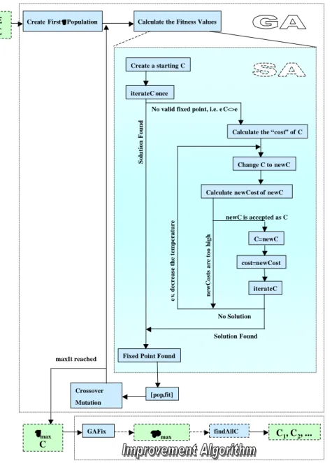
Figure 1 presents a flow-diagram of the combined GASA -algorithm. The doc- umentation to the GASA-Algorithm ((Grohall and Jung, 2003)) contains more detailed information about the functionality of the coded procedures.
6The Main GASA-Routine In a nutshell the routine is doing the following.
The GA-function searches for a maximally stable τ-vector, τ
max, while simulta- neously an SA Algorithm checks whether an accompanying C matrix fulfills the properties of a fixed-point.
7The routine starts with the creation of a population of random τ vectors.
Then we sum up the squared entries of all vectors. These are the according fitness values for the τ population. Next we check for each τ whether we can find a control coefficient matrix C that fulfills the properties of a fixed point. For this we create a random starting C
land plug it into (2). If C
l= C
l+1, we found a fixed point and the fitness value of τ remains equal to the sum of squared entries. If it does not fulfill the constraint in (1), we calculate the “deviation from equality”
or the “costs” as
costs = 1 [C
l− C
l+1]
.21
where 1 are summation vectors. In short, we sum up all the squared entries of the resulting deviation matrix. In the next step we calculate a new random C, C
new. An implicit “temperature” variable determines the randomness we allow for the creation of the new matrix. If temperature is low, the new random matrix is less likely to deviate a lot from the old C matrix. However, if temperature is still high, a completely “different” C
newis very likely. We again calculate the cost of C
newas 1 [C
new,l− C
new,
l+1]
.21.
If costs of C
neware lower than costs of the initial C, we accept C
newas a candidate. If costs of C
neware higher, we do reject C
newwith a certain probability.
This probability depends again on the temperature variable. The probability of rejecting C
newis low at the beginning of the SA-process. The accepted C is then iterated forward as in (2). If we are inside the basin of attraction of a fixed
6
The documentation is available upon request from the authors. Contact:
grohall@ihs.ac.at or jung@ihs.ac.at
7Compare constraint in (2).
point, the iteration of (2) is a quick way to find it. However, if the candidate C lies outside, the iteration does not converge. In the latter case we decrease the temperature variable by 10% and create another C
new. In case we cannot find a fixed point C after a prefixed number of iterations, the fitness value of τ is set to zero and the routine proceeds to the next τ of the population.
Once we repeat this procedure for every τ , we end up having the same, un- changed τ population as before. However, some fitness values will have changed.
In the next step we sort all τ ’s according to fitness and then employ crossover and mutation procedures on the best candidates. This gives us a new population of τ vectors for which we can again calculate fitness values.
Repeating this procedure for several generations of τ populations will results in a large τ
maxvector and an accompanying C matrix that fulfills the properties of a fixed point.
The Improvement Routine In this section we try to improve the results from the last section. We use the bundle τ
maxand C as starting values for an improvement routine. This routine searches much faster for even higher entries in τ
maxwhich still support the equilibrium given the supplied control coefficients in C. Therefore, the algorithm does not need to find an equilibrium, it just checks whether the equilibrium supplied, is still valid with higher values in τ
max. This is done in two steps.
At first, higher entries in τ
maxfor the given C are searched by the GA-function, leaving away the SA-part. We do not need the SA-part since we already have a suitable control coefficient matrix, namely C
∗. The routine increases each single entry in τ
maxone at a time by 1, and then uses the constraint of (1) to check, whether the new τ still respects it. Thus, a maximum ¯ τ
maxis found, when no entry in ¯ τ
maxcan be increased anymore, without violating the constraint in (1).
If good starting guesses exist already, we can use this guess on C and check for the largest possible τ-vector supporting this C as a fixed-point.
After the GA and the special routine delivered the maximally stable ¯ τ
max, we run a search function (findAllC) on it which finds all stable control coefficient matrices C
1, C
2, ... for that vector. Note that the SA routine and the search function of the last paragraph can take extremely long to finish.
4 Applying the Algorithm
Complex ownership structures have been reported to serve as control devices for investor groups or the management (e.g. pyramid structures etc.). Cross- ownership plays a particulary interesting role in control strategies and so far, theory is not able to clearly identify control rights from ownership data, once cross-holding structures are present. Cross-ownership makes it possible for mi- nority shareholders to effectively control large numbers of companies while keep-
8
ing a low profile and stay virtually undetected. In the extreme, it can be shown that under a given ownership structure, even a zero-shareholder who is assigned control rights (a CEO for example) cannot be unseated by the actual owners of the companies. The model by (Ritzberger and Shorish, 2002) allows to identify such controlling individuals using data on interfirm and private shareholding.
Since these private shareholders or better, ultimate owners.
This model employs a very complex nonlinear, multi-objective maximization of a step function. Due to the inherent possibility of coalition building among agents the problem is computationally very expensive, especially when one has to rely on gradient descent methods for continuous problems. Therefore, this model seems to be an ideal candidate for the GASA-algorithm.
In the next section we give a motivating example, similar to the one given in (Ritzberger and Shorish, 2002). Then we employ the GASA-algorithm on one of Germany’s largest firm conglomerates, the “Allianz Group”. The Allianz AG used to have cross-ownership in parts of a very complex firm network. Our data are from the year 2001. Since then, the network got somewhat disentangled and the cross-ownership structure has been broken up by now. However, tests on the older data suggest that given the data restrictions that we face at this point, Bank Austria and AB Industriebesitz- und Beteiligungen AG & Co.KG are strong players in the Allianz network as of 2001. Strong in this sense means, that both firms could be identified as controlling shareholders of a large part of the Allianz conglomerate. In one specification, we could also identify a zero-shareholder who could, in theory, control large parts of the Allianz network.
4.1 A Motivating Example
One of the most intriguing facts about cross-ownership is that individuals holding control rights (i.e. CEOs) in combination with low percentage or no holdings in ownership might be impossible to unseat! They are able to control one or more firms out of the cross-owned group of firms. In the following example we highlight the case of three companies and two individuals, also called ultimate shareholders.
Each company holds 28% of the other and the remaining 44% of each firm are owned by individual 1, who is also the CEO in each firm. To work with a more compact form we summarize the ownership information in two matrices.
Σ =
0 0.28 0.28 0.28 0 0.28 0.28 0.28 0
Ξ =
0.44 0.44 0.44
0 0 0
We call Σ the cross ownership matrix and Ξ the ultimate owner matrix. Its single entries σ
i,jwith i, j = 1,2 or 3, denote the holdings of firm i in firm j.
Likewise, the entry ϑ
i,jin Ξ with i = 1 or 2 and j = 1, 2 or 3 denotes the
percentage of privately owned shares. Note that the columns of Σ and Ξ sum up
to 1, i.e. 100% of the companies are owned. Note also that a firm cannot own its own shares, so the main diagonal of Σ is zero!
In our example we assume that investor 1 (first row in Ξ) is the CEO and controls all firms. In addition she owns the remaining shares, 44% in each firms.
We claim that this investor cannot be unseated. Whatever investor 2 is doing, she cannot unseat the CEO (investor 1). This is a trivial equilibrium and close to what one would expect in view of the high percentage shareholdings of investor 1.
However, let us assume now that investor 2, the person who owns nothing, is the CEO in all three firms. Can investor 2 unseat the CEO if she is unhappy with her performance? Person 2 will use the 28% from firms 2 and 3, where she is also CEO, to block any attack on her position in firm 1. Since she controls 56%
in firm 1, she cannot be unseated as CEO in firm 1 by investor 1. Even though investor 2 does not own a single share, she can use her power in the remaining two firms to protect her control rights. This situation is again an equilibrium!
4.2 The Theoretical Foundations
(Ritzberger and Shorish, 2002) develop a completely new methodology for finding the controlling individual of a company in the event of cross-ownership among firms. Here we briefly introduce their main idea.
Let m be the number of firms and let n be the number of investors. In addition, (Ritzberger and Shorish, 2002) specify an equation system that allows for simultaneous consideration of all firms and investors. The solution to this equation system is a matrix C of control coefficients c
ijfor all i = 1, ..., n and all j = 1, ..., m. These control coefficients are considered to be indicator functions that are strictly positive if and only if investor i can control firm j. If a single investor controls firm j, the according control coefficient equals 1. For all other investors than i, the control coefficients for firm j are zero. This means that investor i has full control over firm j. If, however, several investors, say k, are able to control a firm, i.e. they all control the same amount of shares, their control coefficients for firm j are all equal to 1/k and sum up to 1.
How strong is this control? Against how many other shareholders can control be maintained? These questions are answered by introducing an embedded vector τ, recording coalition sizes (the number of “opposing” investors) against which control can be defended by investor i. In order to write this problem down, we have to define the set of all such coalitions of length t ∈ T = { 1, ..., n − 1 } that could team up against investor i. We denote this set as N
it. If investor i wants to “win” against a coalition of size t, she has to control more votes in that firm than any one of these coalitions N ∈ N
itwhere N ⊂ { 1, ..., n } . Vector τ = (t
1, t
2, ..., t
j, ..., t
m) records these coalition sizes for every firm j, where t
jrecords the coalition size for firm j.
Let us consider the case of a shareholder assembly. The incumbent CEO may
10
be unseated if a coalition of shareholders votes against her. Since the incumbent CEO is not voting against herself the size of this opposing coalition can maximally be, t
j∈ T = 1, ..., n − 1. If the old CEO controls at least 50% of the votes, she will be confirmed as CEO. In fact, it might not even be necessary to control that many shares if not every shareholder joins the votings. If a shareholder considers his costs to be higher than the utility he gains from voting, he will not join.
If a coalition of two investors is enough to unseat the old CEO, we speak of control at relative majority. If a coalition formed of all (n − 1) investors is not able to unseat investor i (the CEO in our example), we speak of control at absolute majority. If a certain number, call it t
j, of investors is necessary to unseat the CEO of firm j , we speak of control at level (or coalition size) t, which could be anything from 1 to n − 1. If, at a certain coalition size t
j, the CEO of firm j cannot be unseated, the system has reached an equilibrium for this particular control coefficient c
ij.
We extend this definition to the whole system and say that if, at certain coali- tion sizes, summarized in the vector τ , all CEOs of all firms cannot be unseated, the system has reached an equilibrium for this particular set of control coefficients, summarized in C. Here is another intuitive definition for this equilibrium:
An equilibrium is a control coefficient matrix C which can not be changed at a shareholder meeting, given a maximum coalition size for each firm. In addition, all firms have to be controlled.
If this is the case, no CEO can be unseated as long as in all companies the coalition size t
jin the election is not surpassed. If a firm is left uncontrolled it might be possible that this firm will be used in the next election to unseat the CEO, thus it would be no real equilibrium. To prevent such cases, all firms have to be controlled, eC = e, that is, the sum of each column in C has to be 1.
To calculate control over a company, we define the space of shares in a given firm that are potentially under the control of investors, as ∆ =
x ∈ R
+n| ex ≤ 1 , with x ∈ ∆ and i = 1, ..., n being the number of ultimate owners. Therefore, x is a column vector of positive values which sum up to a number smaller or equal 1.
These values represent the percent-shareholdings of the n investors in one specific firm.
Now (Ritzberger and Shorish, 2002) define a step function f
it(x) : ∆ → R
+which is applied to each i, resulting in a control coefficient for each investor in the company. They prove that this function is necessary and sufficient to determine the control coefficients. Next they extend this analysis to the whole system. The matrix X
n×m= [x
1. . . x
m] represents the control coefficients where each column represents one firm. Now apply F
τ(X) : ∆
m→ ∆
m:
F
τ(X) =
f
τ(1)(x
1) . . . f
τ(m)(x
m)
where f
tis applied to each single entry of matrix X.
The matrix of voting shares controlled by the different investors is given by X = Ξ + CΣ, where C is a set of control coefficients in equilibrium fulfilling F
τ(Ξ + CΣ) = C and eC = e, which is the control equilibrium together with a maximized vector τ = [τ(1) . . . τ (m)] ∈ T
m.
This definition interprets the problem as a fixed point search. The function F
τ(X) maps the actual set of control coefficients into a new such set. If none of the CEOs can be unseated against their will, the resulting new set will be equal to the old one and an equilibrium has been found. This equilibrium is called maximally stable, if increasing the coalition size for any firm leads to unstable companies. This means that the firm’s CEO can always be voted out. (Ritzberger and Shorish, 2002) prove that such a maximally stable control equilibrium exists for every pair of ownership matrices Ξ and Σ. It can also be the case that multiple control equilibria exist, as was shown in the example at the beginning of the chapter.
4.3 Data Description
The core of the data is from the Commerzbank CD-ROM of the year 2001. We complete the data with data from the annual reports of Allianz AG, Deutsche Bank AG, M¨ unchener R¨ uckversicherung, Dresdner Bank and Bayerische Hypo- und Vereinsbank of the same year whenever applicable. The database includes shareholdings of firms and private owners down to 0.1% holdings.
To account for missing data and dispersed ownership we generate two distinct data pools for every data set. The first treats dispersed owners as one single shareholder. That means that the data counts them as blocks. E.g.: The 31%
dispersed ownership of a company are treated as if those investors were one person. The residual unknown holdings (i.e. if data is not complete there is a residual percentage of unknown shareholders) are ignored. This dataset is called FabFive.
In the second pool we augment the identified dispersed ownership block with the unknown residual ownership percentage that is not included in our data.
Furthermore, we assume that the smallest single (dispersed) shareholder unit is 0.001%. Thus, in order to control 1% of the company one needs 1000 of such units. This implies that the 31% dispersed shareholder block consists of 31000 single shareholders. This treatment will increase coalition lengths considerably in later computations. This dataset is called FabFiveDisp.
Finally, we increase our dataset by adding firms which are typically not said to be in the core of the Allianz-Group, but which own shares in at least one of the five main firms. The resulting pools of data are called Network and NetworkDisp.
These datasets represent every direct and indirect ownership in one of the Allianz- Group firms.
12
4.4 The FabFive Results
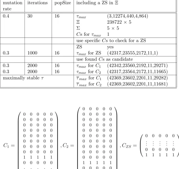
The FabFive set includes data on the Allianz, the Deutsche Bank, the M¨ unchener R¨ uckversicherung and the Bayerische Hypo- und Vereinsbank. This is the core crossholding network. The data includes 16 ultimate shareholders and 5 firms.
These numbers represent ownership data between the 97% to 100% range for each of the big five firms. The only outlier is the Bayerische Hypo- und Vereinsbank for which only 88.16% of the ownership data are available at this point.
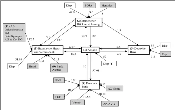
8Figure 2 represents this firm conglomerate graphically.
4.4.1 Dispersed Shareholders Treated as One Single Voter
Table 1 summarizes the results for the FabFive dataset. ZS is the abbreviation for zero-shareholder, a person owning nothing, but controlling everything
Table 1: FabFive – Dispersed Shareholders Treated as One Single Blockholder mutation
rate
iterations popSize including a ZS in Ξ
0.4 30 16 τ
max(15,2,15,15,1)
Ξ 16 × 5
Σ 5 × 5
Cs for τ
max1
use specific Cs to check for the ZS
ZS no
0.3 100 16 τ
maxfor ZS no
use found Cs as candidate
0.4 100 16 τ
maxfor C (15,2,15,15,1)
The control coefficient matrix C the algorithm found for the τ
max= (15, 2, 15, 15, 1) is:
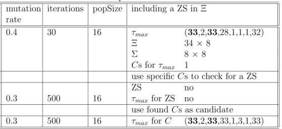
9C
16×5=
1 0 0 1 0 0 1 0 0 0 0 0 1 0 0 0 0 0 0 1 0 0 0 0 0 .. . .. . .. . .. . .. .
(9)
8
Later we can increase this percentage to 94.76% in the Network dataset.
9The bold entries in τ are fixed entries of maximum coalition size, n-1. A specific ultimate shareholder holds more than 50% in these firms and therefore controls them from the start at majority level.
The first ultimate shareholder – this is the dispersed owners block holding 57%
called Disp in Figure 2 – controls firm 1 (Allianz AG) at absolute majority. The maximum coalition length possible in this case is 15, given the dimension of the Ξ matrix indicating a total number of 16 ultimate shareholders. The same shareholder-block also controls firm 4 (Dresdner Bank) through her control over firm 1 (Allianz AG). This control is again maintained at the absolute majority level, since firm 1 (Allianz AG) owns 57.68% in firm 4 (Dresdner Bank). This already covers control for firm 1 and firm 4.
The second ultimate shareholder – the dispersed owners block holding 44.9%
in firm 2 (M”unchener R”uckversicherung) – is again denoted as Disp in Figure 2. This block controls firm 2 (M”unchener R”uckversicherung) at a coalition length of two. This means that at least a coalition of three other shareholders is necessary to oust ultimate holder 2 from control.
Firm 3 (Deutsche Bank) is controlled at absolute majority by the 89% block of dispersed owners and firm 5 (Bayerische Hypo- und Vereinsbank) is controlled by the dispersed block holding 31.84% at the relative majority level.
10Using a pre-specified control coefficient matrix representing the zero-shareholder who controls the entire group and using it as input for the two-step optimiza- tion routine does not indicate the existence of such a shareholder. The values given in Table 1 are those found by the GASA-algorithm. The improvement al- gorithm does not find any higher values here, leading to the conclusion that for this small example, the GASA-algorithm was good enough to find the precise global optimum.
4.4.2 Dispersed Shareholders treated as Single Voters
Table 2 reports the result for the FabFiveDisp dataset which treats the dispersed shareholder blocks from the last section plus the remaining (missing) ownership percentage as many single dispersed shareholders each holding 0.001% of the re- spective firm’s shares. The values of τ
maxare those found by the GASA-algorithm, while those called τ
maxare global optima, found by the improvement algorithm using τ
maxas starting value.
The resulting candidate matrices for τ
max= (3, 12274, 440, 4, 864) are of di- mension 238722 × 5:
10Relative majority level is coalition length of one in the τmax vector. That means that a coalition of two other shareholders is already able to unseat the controlling shareholder.
14
Table 2: FabFiveDisp – Dispersed Shareholders Treated as Single Persons mutation
rate
iterations popSize including a ZS in Ξ
0.4 30 16 τ
max(3,12274,440,4,864)
Ξ 238722 × 5
Σ 5 × 5
Cs for τ
max1
use specific Cs to check for a ZS
ZS yes
0.3 1000 16 τ
maxfor ZS (42317,23555,2172,11,1) use found Cs as candidate
0.3 2000 16 τ
maxfor C
1(42342,23560,2192,11,29271) 0.3 2000 16 τ
maxfor C
2(42317,23564,2172,11,11665) maximally stable τ τ
maxfor C
1(42369,23602,2201,11,29282) τ
maxfor C
2(42369,23602,2201,11,11681)
C
1=
0 0 0 0 0
0 0 0 0 0
0 0 0 0 0
0 0 0 0 0
0 0 0 0 0
0 0 0 0 0
0 0 0 0 0
0 0 0 0 0
1 1 1 1 1
0 0 0 0 0
... ... ... ... ...
0 0 0 0 0
, C
2=
0 0 0 0 0
0 0 0 0 0
0 0 0 0 0
0 0 0 0 0
0 0 0 0 0
0 0 0 0 0
0 0 0 0 0
0 0 0 0 0
0 0 0 0 0
0 0 0 0 0
1 1 1 1 1
0 0 0 0 0
... ... ... ... ...
0 0 0 0 0
, C
ZS=
0 0 0 0 0
... ... ... ... ...
0 0 0 0 0
1 1 1 1 1
These matrices indicate that either firm 9 (AB holding 12.5% in the Bayerische Hypo- und Vereinsbank) or firm 11 (BA holding 21.3% in the Bayerische Hypo- und Vereinsbank) can control the conglomerate at coalition lengths represented in τ
max.
11In addition, we are able to identify a zero-shareholder who can control the entire conglomerate at considerable coalition lengths τ
max= (42317, 23555, 2172, 11, 1).
After using the two candidate matrices C
1and C
2in the faster tow-step op- timization, we can show that much higher coalition lengths for the candidate control coefficient matrices can be sustained. After the first step (using the GA on the fixed C), the initial τ
max= (3, 12274, 440, 4, 864) is increased to τ
max= (42342, 23560, 2192, 11, 29271) for C
1and to τ
max= (42317, 23564, 2172, 11, 11665) for C
2. Here we get a first indication of how effective the faster algorithm works.
11
For details compare Figure 2.
The second part (stepwise increasing every entry in τ
max) finds the control equilibrium (C, τ
max), which is maximally stable. If we would increase any entry by 1, we would immediately destroy the equilibrium and C would not be a fixed- point anymore. Comparing the resulting entries in τ
maxwith the entries in τ
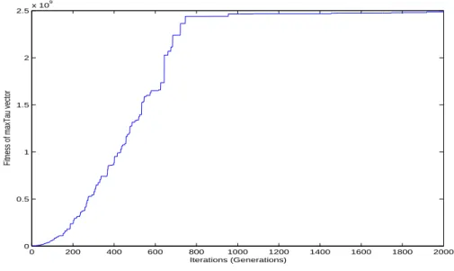
maxwe clearly see that the GA-algorithm produces very good approximations after about 2000 iterations. The stepwise increase makes only sense with good starting values, since it may take very long otherwise. Had we used it from the start onwards, we would have run into combinatorial problems and could not have solved the maximization in due time. Figure 3 gives an idea of the convergence process for C
1and its corresponding τ
max= (42342, 23560, 2192, 11, 29271). The y-axes depicts | τ
max|
2, the fitness value of τ
max.
We see that after about 1200 iterations the fitness value is not changing much anymore. A maximum iteration of 2000 seems to give a good convergence re- sult. In Figure 4 we plot the convergence process for C
2and its corresponding τ
max= (42317, 23564, 2172, 11, 11665). Figure 4 seems to indicate that maybe more iterations would be needed to get more exact results. However, big jumps are not to be expected after about iteration 1200, as in the earlier case.
4.5 The Network Results
In this section we add some firms and thus also some ultimate shareholders.
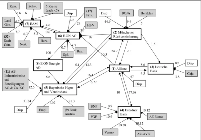
Figure 5 describes the new situation graphically. The additional firms are E.ON Energie AG, E.ON AG and EAM, plus their ultimate shareholders. The rest of the data are the same as in the previous section. The data now includes now 29 ultimate shareholders and 8 firms. Note that no other firms and persons reported in the dataset have direct or indirect holdings in any of the companies in the Network.
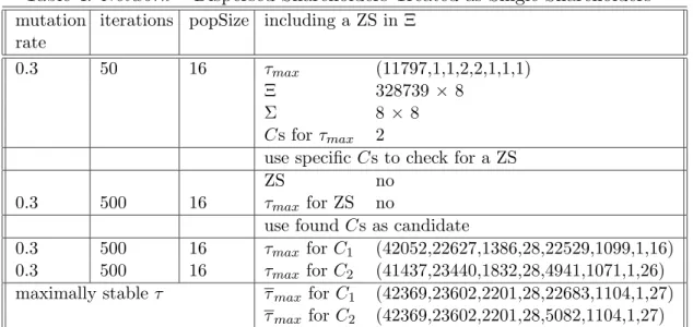
4.5.1 Dispersed Shareholders Treated as One Block Table 3 contains the results in their usual form.
The candidate matrix for τ
max= (33, 2, 33, 28, 1, 1, 1, 32) is:
sparse(C) =
(1, 1) 1 (2, 2) 1 (3, 3) 1 (1, 4) 1 (4, 5) 1 (17, 6) 1 (32, 7) 1 (17, 8) 1
(10)
16
Table 3: Network – Dispersed Shareholders Treated as One Block mutation
rate
iterations popSize including a ZS in Ξ
0.4 30 16 τ
max(33,2,33,28,1,1,1,32)
Ξ 34 × 8
Σ 8 × 8
Cs for τ
max1
use specific Cs to check for a ZS
ZS no
0.3 500 16 τ
maxfor ZS no
use found Cs as candidate
0.3 500 16 τ
maxfor C (33,2,33,33,1,3,1,33)
This matrix is in its sparse-form. This is a Matlab command that allows for easy representation of matrices mainly containing zero entries. The numbers in parenthesis indicate the position inside the matrix, read as (row,column), and the number to the right of it is the according value of the matrix at that position.
So at eight positions the matrix has value one and everywhere else the entries are zero.
The first five rows in (10) are the same as in (9) on page 13. That means that we find the same controlling shareholders – as identified for the FabFive dataset – control firms 1 to 5 in the enlarged Network dataset. The additional companies, firm 6 (E.ON AG) and firm 8 (E.ON Energie AG) are controlled by ultimate shareholder 17, which is the 23% shareholder denoted Priv. in Figure 5. Firm 7 (EAM – Energie Aktiengesellschaft Mitteldeutschland) is controlled by shareholder 32 (Stadt G¨ ottingen) which holds 7.7% in EAM shares. There is no indication of a zero-shareholder controlling the entire group.
Again, using the first step of the optimization routine, we get a slightly higher τ
maxthan the original one. From this vector we conclude that firms 1,3,4 and 8 are controlled at absolute majority. The rest is controlled at lower coalition lengths. Once we compare the respective τ
maxvectors in Table 1 for the FabFive dataset and Table 3 for the Network dataset we see that the first five firms are controlled at exactly the same coalition sizes.
12Firm 8 (E.ON Energie AG) is controlled at absolute majority by firm 6 (E.ON AG) which is controlled by ultimate shareholder 17 (Priv.) at coalition size 3.
Firm 7 (EAM) is only controlled at relative majority (coalition size equal to one) by ultimate shareholder 32 (Stadt G¨ ottingen).
12Compare τmax = (15,2,15,15,1) and the second τmax = (33,2,33,33,1,3,1,33). Since we are dealing with 34 ultimate shareholders in the second case, 33 represents the maximum coalition length in the second case, which corresponds to the 15 maximum coalition size in the first case.
In this case, the GASA-algorithm does not result in the global optimum, but the first step of the optimization function is enough to find τ
maxsince stepwise increasing the entries does not lead to higher stable coalition sizes.
4.5.2 Dispersed Shareholders treated as Single Voters
Similar as in Section 4.4.2, Table 4 reports the result for the NetworkDisp dataset which treats the dispersed shareholder block from the last section plus the re- maining (missing) ownership percentage as many single dispersed shareholders each holding 0.001% of the respective firm’s shares.
Table 4: Network – Dispersed Shareholders Treated as Single Shareholders mutation
rate
iterations popSize including a ZS in Ξ
0.3 50 16 τ
max(11797,1,1,2,2,1,1,1)
Ξ 328739 × 8
Σ 8 × 8
Cs for τ
max2
use specific Cs to check for a ZS
ZS no
0.3 500 16 τ
maxfor ZS no
use found Cs as candidate
0.3 500 16 τ
maxfor C
1(42052,22627,1386,28,22529,1099,1,16) 0.3 500 16 τ
maxfor C
2(41437,23440,1832,28,4941,1071,1,26) maximally stable τ τ
maxfor C
1(42369,23602,2201,28,22683,1104,1,27)
τ
maxfor C
2(42369,23602,2201,28,5082,1104,1,27) The resulting candidate matrices for τ
max= (11797, 1, 1, 2, 2, 1, 1, 1) are again given in spares-notation and of dimension 328739 × 8:
sparse(C
1) =
(9, 1) 1 (9, 2) 1 (9, 3) 1 (9, 4) 1 (9, 5) 1 (17, 6) 1 (32, 7) 1 (17, 8) 1
sparse(C
2) =
(11, 1) 1 (11, 2) 1 (11, 3) 1 (11, 4) 1 (11, 5) 1 (17, 6) 1 (32, 7) 1 (17, 8) 1
From C
1we see that ultimate shareholder 9 (Bank Austria) is able to control firm 1 to 5 at various coalition sizes. Firm 6 (E.ON AG) and firm 8 (E.ON Energie AG) are still controlled by ultimate shareholder 17 (Priv.) as in the
18
Network dataset. Firm 7 (EAM – Energie Aktiengesellschaft Mitteldeutschland) is controlled by ultimate shareholder 32 (Stadt G¨ ottingen).
The matrix C
2indicates that ultimate shareholder 11 (AB Industriebesitz und Beteiligungen AG & Co. KG) controls firm 1 to 5. Firm 6 to 8 are con- trolled by the same shareholders as before. In addition, we could not find a zero-shareholder controlling the whole structure. Running the first part of the optimization-routine considerably increases the coalition sizes for the two con- trol coefficient matrices C
1and C
2. Comparing these results with the absolutely highest coalitions sizes possible, τ
max, indicates again at very strong convergence results after 2000 iterations.
5 Conclusion
We have shown that using a numerical technique, combining Genetic Algorithms
with Simulated Annealing routines, allows us to overcome traditional computa-
tional pitfalls in maximizing a multi-objective step function. We demonstrate
results that are good approximations to the true values that theory predicts for
small sample cases. Furthermore, we extend our analysis to real world data on
firm ownership in Germany. We solve a particular model by (Ritzberger and
Shorish, 2002) and present evidence of two very powerful shareholders within the
Allianz group. These findings are based on data of the year 2001 and underly the
assumptions of the model in (Ritzberger and Shorish, 2002).
References
Chipperfield, A., Fleming, P., Pohlheim, H., and Fonseca, C. (1999). Genetic Al- gorithm Toolbox, For Use with MATLAB. Department of Automatic Control and Systems Engineering, University of Sheffield, 1.2 edition.
Grohall, G. and Jung, J. (2003). Genetic Algorithm and Simulated Annealing MatLab-Code Documentation. Institute for Advanced Studies, Vienna.
Metropolis, N., Rosenbluth, A., Rosenbluth, M., Teller, A., and Teller, E. (1953).
Equation of state calculations by fast computing machines. Journal of Chem.Physics, 21:1087 – 1092.
Moins, S. (2002). Implementation of a simulated annealing algorithm for Matlab.
Link¨ oping Institute of Technology.
Ritzberger, K. and Shorish, J. (2002). The building of empires: Measuring the separation of dividend and control rights under cross-ownership among firms.
Version from November 2002.
Wu, L. and Wang, Y. (1998). An introduction to simulated annealing algorithms for the computation of economic equilibrium. Computational Economics, 12(2):151–169.
20
Figure 1: The GASA Algorithm
Create a starting C
iterateC once
Calculate the “cost” of C
Change C to newC
Calculate newCost of newC
C=newC
cost=newCost
iterateC No valid fixed point, i.e. e C<>e
No Solution
newC is accepted as C
Fixed Point Found
Solution Found Solution Found ev. decrease the temperature
Create FirstττPopulation Calculate the Fitness Values
[pop,fit]
Crossover Mutation
τ τmax
C
maxIt reached
Ξ Σ
newCostsare too high
GAFix ττττ∗∗∗∗max findAllC C1, C2, ...
Figure 2: FabFive
(1)Allianz (3) Deutsche
Bank
(4)Dresdner Bank (2) Münchener Rückversicherung
(5)Bayerische Hypo- und Vereinsbank
Disp
Disp (1) Disp
Disp
Caja
AZ-Noma
AZ-AVG Vermo
FGF Empl
(11) AB Industriebesitz und Beteiligungen AG & Co. KG
(9)Bank Austria
BOJA Herakles
1.5
5.6 4.5
89
3.8 9.6 5
44.9
20 24.9
57
10
10.12
10.12 10.58
10.6
BNP 0.9
6.77 16.4 13.3 5.1
1.02 21.3 31.84
12.5
57.68
Figure 3: FabFiveDisp – Convergence for τ
maxof C
10 200 400 600 800 1000 1200 1400 1600 1800 2000
0 0.5 1 1.5 2 2.5 3 3.5x 10⁹
Iterations (Generations)
Fitness of maxTau vector
22
Figure 4: FabFiveDisp – Convergence for τ
maxof C
20 200 400 600 800 1000 1200 1400 1600 1800 2000
0 0.5 1 1.5 2 2.5x 10⁹
Iterations (Generations)
Fitness of maxTau vector
Figure 5: Network
(1)Allianz (3) Deutsche Bank
(4)Dresdner Bank (2) Münchener Rückversicherung
(5)Bayerische Hypo- und Vereinsbank
Disp
Disp Disp
Disp
Caja
AZ-Noma
AZ-AVG Vermo
FGF Empl
(11) AB Industriebesitz und Beteiligungen AG & Co. KG
(9) Bank Austria
BOJA Herakles
1.5
5.6 4.5
89
3.8 9.6 5
44.9
20 24.9
57
10
10.12
10.12 10.58
10.6
BNP 0.9
6.77 16.4 13.3 5.1
1.02 21.3 31.84
12.5
(6) E.ON AG
(8) E.ON Energie AG
(7) EAM
Disp
HI-V (17) Priv.
Bay.
Syd.
07 0.7 5.7
3.7 23 4.6
100 5 Kreise (each <5) Schw.
Kass.
Land Gött.
Nort.
Hers.
6.7 5.3 4.7
7.7 6.6 6
4.6 0.6
6.6
10.5
57.68 (32)
Stadt Gött.