Lessons for Loss Given Default, Lifetime Expected Loss and Bank Capital Requirements
A dissertation in partial fulfillment of the requirements for the degree of Doktor der Wirtschaftswissenschaft (Dr. rer. pol.)
submitted to the
Faculty of Business, Economics, and Management Information Systems Universität Regensburg
submitted by Steffen Krüger
Advisors:
Prof. Dr. Daniel Rösch Prof. Dr. Alfred Hamerle
Date of the Disputation: August 23, 2017
I would like to thank Prof. Dr. Daniel Rösch for his continuous support of my doctoral thesis and his motivation, enthusiasm, and patience. His guidance and immense knowl- edge have been invaluable. I gratefully acknowledge Prof. em. Dr. Alfred Hamerle to be my second advisor.
The chapters of this thesis would not have been possible without the fruitful collaboration with several co-authors and colleagues. I want to express my gratitude to Prof. Dr. Harald Scheule for his expertise and the invitation to his university. I would like to thank Jennifer Betz for the great time we had when we shared an office.
Last but not least, I would like to thank my family and friends for their ongoing support.
I am forever indebted to my mother and to Juli for all their love and encouragement.
List of Tables v
List of Figures vii
1 Introduction 1
2 Downturn LGD Modeling using Quantile Regression 12
2.1 Introduction . . . . 13
2.1.1 Motivation and Literature . . . . 13
2.1.2 Introductory Example . . . . 15
2.2 Modeling Loss Given Default . . . . 17
2.2.1 Quantile Regression . . . . 17
2.2.2 Simulation Study . . . . 18
2.2.3 Comparative Methods . . . . 21
2.3 Data . . . . 23
2.4 Empirical Analysis . . . . 27
2.4.1 Quantile Regression . . . . 27
2.4.2 Model Comparison . . . . 31
2.5 Implications . . . . 35
2.5.1 Loss Distribution . . . . 35
2.5.2 Downturn LGDs . . . . 38
2.6 Conclusion . . . . 42
Appendix 2.A Quantile Regression . . . . 43
Appendix 2.B Comparative Methods . . . . 44
Appendix 2.C Macroeconomic Variables . . . . 46
3.1 Introduction . . . . 49
3.2 Why Care about Systematic Effects among Default Resolution Times? . 52 3.3 Methods and Data . . . . 57
3.3.1 Methods . . . . 57
3.3.2 Data . . . . 60
3.4 Results . . . . 66
3.4.1 Overview of Formal and Informal Proceedings of Resolution . . . 66
3.4.2 Loan Specific Impacts on Resolution . . . . 70
3.4.3 The Systematic Movement of Resolution Processes . . . . 73
3.5 Implications of Systematic DRTs . . . . 86
3.5.1 Implications on Loan Level . . . . 87
3.5.2 Implications on Portfolio Level . . . . 91
3.6 Conclusion . . . . 95
Appendix 3.A Estimation of the Cox Model . . . . 97
Appendix 3.B Further Outputs . . . . 99
3.B.1 Covariate Influences over Time . . . . 99
3.B.2 Joint Country Regression . . . . 104
3.B.3 Regression Results for Additional Macroeconomic Variables . . . . 107
4 A Copula Sample Selection Model for Predicting Multi-Year LGDs and Lifetime Expected Losses 108 4.1 Introduction . . . . 109
4.2 Model . . . . 111
4.2.1 Multi-Year Losses over Lifetime . . . . 111
4.2.2 Default Time Model . . . . 113
4.2.3 Loss Given Default Model . . . . 114
4.2.4 Copula Selection Model . . . . 116
4.3 Empirical Analysis . . . . 118
4.3.3 Marginal Models . . . . 124
4.3.4 Copula Models . . . . 129
4.4 Applications . . . . 129
4.4.1 The Term Structure of LGDs . . . . 129
4.4.2 Estimation of Lifetime Expected Losses . . . . 132
4.5 Conclusion . . . . 135
Appendix 4.A Copula Theory . . . . 137
4.A.1 Introduction . . . . 137
4.A.2 Densities . . . . 138
4.A.3 Properties . . . . 139
Appendix 4.B Empirical Robustness Tests . . . . 140
5 The Impact of Loan Loss Provisioning on Bank Capital Requirements 142 5.1 Introduction . . . . 143
5.2 Capital Requirements and Provisioning . . . . 144
5.2.1 Accounting Provisions . . . . 145
5.2.2 Basel Expected Loss and Capital Requirements . . . . 146
5.3 Data . . . . 149
5.3.1 Issuer- and Bond-Specific Covariates . . . . 149
5.3.2 Cyclical Behavior . . . . 152
5.4 Loan Loss Provisioning . . . . 154
5.4.1 12-month Expected Loss for Basel and IFRS 9 (Stage 1) . . . . . 154
5.4.2 Lifetime Expected Loss for GAAP 326 and IFRS 9 (Stage 2) . . . 159
5.4.3 Significant Increase in Credit Risk (SICR) . . . . 163
5.5 Impact on Regulatory Capital . . . . 165
5.5.1 Stylized Asset Portfolios . . . . 165
5.5.2 Significant Increase in Credit Risk (SICR) . . . . 167
5.5.3 Computation of Basel and Accounting Expected Losses . . . . 169
Appendix 5.A The Performance of Macroeconomic Variables . . . . 180
6 Conclusion 183
References 189
2.1 Exemplary Downturn Loss Rates Given Default . . . . 17
2.2 Simulation – Data generation . . . . 19
2.3 Comparative methods . . . . 22
2.4 Descriptive statistics . . . . 26
2.5 Parameter estimates Quantile Regression . . . . 28
2.6 In-sample goodness of fit . . . . 31
2.7 Out-of-sample goodness of fit . . . . 34
2.8 Hit rates of VaR based Downturn LGD . . . . 38
2.B.1 Parameter estimates comparative methods . . . . 45
2.C.1 Effects of macroeconomic information in the first year of resolution, i.e. after default . . . . 46
3.1 Descriptive statistics of DRT . . . . 61
3.2 Descriptive statistics of loan specific characteristics . . . . 64
3.3 Pairwise correlations of macroeconomic variables . . . . 65
3.4 Overview of formal and informal proceedings . . . . 67
3.5 Regression results for Model I . . . . 71
3.6 Regression results for Model II . . . . 78
3.7 Regression results for Model III . . . . 82
3.8 Frailty impact on mean DRT . . . . 83
3.9 Inferences of systematic factors on the distribution of DRTs . . . . 90
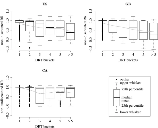
3.10 Non-discounted RR by DRT buckets . . . . 91
3.11 Inferences of systematic factors on the distribution of portfolio DRTs . . . 92
3.B.1 Regression results for Model III when including interactions of covariates
and recessions: parameter estimates non-recession . . . . 100
3.B.3 Regression results for Model I, II and III across countries . . . . 105
3.B.4 Regression results for Model II with different macroeconomic variables . . 107
4.1 Descriptive statistics of bond- and issuer-specific information (1) . . . . . 121
4.2 Descriptive statistics of bond- and issuer-specific information (2) . . . . . 122
4.3 Descriptive statistics of exemplary risk-buckets . . . . 124
4.4 Parameter estimates for the time-to-default . . . . 126
4.5 Parameter estimates for the loss given default . . . . 128
4.6 Parameter estimates for the copula . . . . 129
4.7 LEL predictions for industrial bonds . . . . 134
4.A.1 Copula properties . . . . 139
4.B.1 Copula performance . . . . 140
4.B.2 Default model performance . . . . 141
5.1 Exemplary calculation of regulatory capital . . . . 148
5.2 Descriptive statistics for issuer- and bond-specific covariates . . . . 151
5.3 Parameter estimates Probability of Default . . . . 155
5.4 Parameter estimates Loss Rate Given Default . . . . 158
5.5 Parameter estimates AR model . . . . 160
5.6 Credit quality distributions of stylized portfolios . . . . 165
5.7 Deduction of Common Equity Tier 1 due to provisioning . . . . 174
5.8 Deduction of CET 1 for different reinvestment strategies . . . . 176
5.A.1 Macroeconomic variables . . . . 180
5.A.2 Regression results for additional macroeconomic variables . . . . 181
5.A.3 Deduction of CET 1 using alternative macroeconomic variables . . . . . 182
2.1 Stylized LGD Distributions . . . . 16
2.2 Simulation – Data generation . . . . 19
2.3 Simulation – Parameter estimation . . . . 20
2.4 Simulation – Forecasting . . . . 21
2.5 Observed Loss Rates Given Default . . . . 24
2.6 Loss Rates Given Default over time . . . . 25
2.7 In-sample goodness of fit (R
1) . . . . 32
2.8 In-sample goodness of fit (P-P plot) . . . . 33
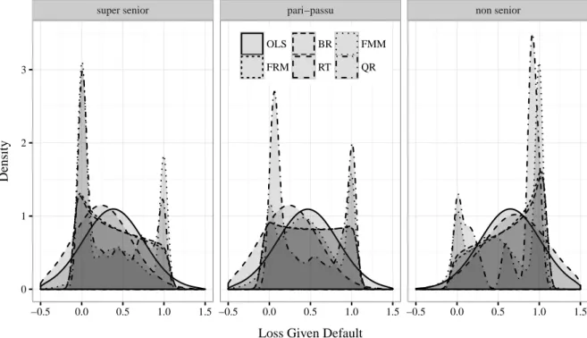
2.9 Densities of Loss Rates Given Default . . . . 36
2.10 Predictions of the Value at Risk (VaR) . . . . 37
2.11 Densities of Loss Rates Given Default during the economic cycle . . . . . 40
2.12 Downturn effects on LGD quantiles . . . . 41
2.13 Predictions of Quantile Regression based Downturn LGDs . . . . 41
2.A.1 Parameter estimates Quantile Regression . . . . 43
2.B.1 Estimated Regression Tree . . . . 44
3.1 Systematic movements in DRTs . . . . 53
3.2 Relation of DRT and non-discounted RR . . . . 54
3.3 Additional required amount of stable funding . . . . 56
3.4 Resolution time levels . . . . 59
3.5 Observed resolution rates . . . . 62
3.6 Descriptive statistics of macroeconomic variables . . . . 66
3.7 Baseline intensities of resolution . . . . 75
3.8 Time-dependent frailties as systematic components of resolution . . . . . 84
3.10 Density of DRT . . . . 90
3.11 Kernel density estimates of loss on portfolio level . . . . 93
3.12 Mean and VaR(95%) of loss on portfolio level . . . . 95
3.B.1 Frailties when including interactions of covariates and recessions . . . . . 99
3.B.2 Frailty for joint country regression . . . . 104
4.1 Histogram of sample LGDs . . . . 119
4.2 Sample default rates and mean LGDs . . . . 120
4.3 Macroeconomic variables . . . . 122
4.4 Scatter plots of realized LGDs and corresponding times-to-default . . . . 123
4.5 Densities of LGDs . . . . 131
4.6 Term structure of PD and LGD . . . . 132
5.1 The meaning behind capital and provisions . . . . 145
5.2 Empirical distribution of Losses Given Default . . . . 150
5.3 Default rates and mean realized Losses Given Default . . . . 153
5.4 Mean predicted Probability of Default . . . . 156
5.5 Mean predicted Loss Given Default . . . . 159
5.6 VIX and corresponding ACF and PACF plot . . . . 160
5.7 Portfolio share of Stage 2 instruments in IFRS 9 . . . . 168
5.8 Provisions and expected losses . . . . 171
5.9 Deduction of the Common Equity Tier 1 due to provisioning . . . . 173
Introduction
Motivation
Financial institutions play a major role for the economy since they ensure the supply of money by lending to corporations, sovereign entities and consumers (cf. Kishan and Opiela (2000) and Gambacorta and Shin (2016)). As financial intermediaries they fulfill at least three functions to match conflicting needs of borrowers and lenders (see e.g., Freixas and Rochet (2008) p. 4). Maturity transformation involves the conversion of short-term liabilities to long-term assets, e.g., deposits to loans. Size transformation encompasses the pooling of small amounts mainly from savers to large amounts for borrowers. Fur- thermore, financial institutions perform risk transformation, e.g., by diversification, and help to reduce the risk for single lenders. The matching of conflicting needs is subject to the risk of imbalances, e.g., payment difficulties of borrowers can prevent banks to fulfill their own liabilities. Therefore, financial institutions need to hold adequate capital reserves to protect themselves against credit risk (cf. Kim and Santomero (1988)). From an overall economic perspective, a distressed financial sector can lead to a reduction of lending. This can extend or intensify economic downturns, as corporations, sovereign entities and consumers are particularly in these times dependent on intermediaries. In extreme cases, a credit crunch can even cause a recession (cf. Akhtar (1994), Sharpe (1995) and Ivashina and Scharfstein (2010)). A professional measurement of the risk to which financial institutions are exposed to is a substantial basis to determine adequate capital reserves (cf. Sharpe (1978) and Dewatripont and Tirole (1994) p. 218 f.).
The management of financial institutions’ capital reserves is subject to several diffi-
culties. For instance, there are incentives to lower reserves in expansions, e.g., to invest
more money in order to increase returns, which can promote capital shortfalls in reces- sions (cf. Gambacorta and Mistrulli (2004)). In addition, the measurement of credit risk is a challenging task and requires the use of sophisticated statistical methods. Even small mistakes in the evaluation of systematic risk, which substantially affects the credit risk with respect to recessions, can lead to severe misjudgments (cf. Kuo and Lee (2007), Duffie et al. (2009), Bade et al. (2011) and Rösch and Scheule (2014)).
Financial regulation can improve the capitalization of financial institutions by mini- mum capital requirements and minimum supervisory requirements to risk management.
The Basel Committee on Banking Supervision (1988, 2006, 2011) subsequently elabo- rated three international frameworks to standardize and extend risk precaution across countries as well as institutions. The Basel Committee was founded as a response to the Herstatt liquidation in 1974, and in 1988 it recommended capital requirements on debt instruments based on the underlying credit risk (Basel I). The first Accord distinguished risk weights between different types of assets but did not account for differences within a given category. As a result, institutions were able to hold riskier assets without having to fulfill higher capital requirements (cf. Basel Committee on Banking Supervision (1999), Hull (2015) p. 336, and Baesens et al. (2016) p. 7). This was one of the reasons for the substantial revision of the framework. Basel II introduced the internal ratings-based ap- proach that enables financial institutions to estimate credit risk by their own statistical models. In addition, it extended capital requirements to operational and market risk, and introduced rules for supervisory review and market discipline. The latest revision (Basel III) is currently being introduced as a response to the global financial crises starting in 2007. Current discussion and consultation papers of financial regulatory authorities show that the development of the regulatory framework is still far from being completed, e.g., Basel Committee on Banking Supervision (2015b, 2016a, 2017) and European Banking Authority (2017).
Credit risk provides the largest share on regulatory capital requirements. For instance,
the latest Risk Assessment Report of the European Banking Authority (2016b) identifies
that 80.5 % of the risk-weighted assets of 131 major EU banks were attributable to credit
risk as of June 30, 2016. Credit risk of a financial instrument can be characterized by three risk parameters that are generally modeled as stochastic variables. The probability of default (PD) denotes the probability that a borrower will not fulfill his payment obli- gations in a given future time period. The loss given default (LGD) specifies the share of the outstanding debt that is lost due to default. The exposure at default (EAD) denotes the outstanding amount. Increased credit losses during economic downturns empirically show co-movements between risk parameters of a single instrument and those of several borrowers. This thesis focuses on the modeling of dependencies in credit risk which is par- ticularly crucial for adequate risk precaution prior to recessions and discusses implications on bank capital requirements. The analyses cover, amongst others, the measurement and statistical modeling of systematic effects on the LGD and workout processes, and the co-movement of PDs and LGDs.
Literature
The statistical modeling and estimation of risk parameters play a major role in the literature on credit risk. On the one hand, recent studies examine determinants of credit risk which includes information on the underlying debt instrument and the borrower.
However, clustered defaults and higher losses during recessions are caused by systematic risk factors, i.e., observable covariates such as macroeconomic variables and unobservable time-varying risk factors. This motivates research on downturn effects and co-movements of risk parameters. Workout processes of defaulted debt also are of particular interest as they are characterized by a high degree of heterogeneity and determine realized losses.
Capital reserves basically are supposed to reduce the risk of financial distress for financial institutions. However, legal requirements can strengthen the burden to raise capital in recessions due to higher regulatory needs.
There are many papers dealing with the default risk of borrowers and financial in-
struments. The structural model of Merton (1974) assumes a stochastic process for the
value of a company and provides a formula for the probability that its value is less than
its debt. In contrast, the following studies use reduced form models and directly model
the default event dependent on explanatory variables. The Z-score of Altman (1968) represents a formula to predict the probability of corporate bankruptcies based on firm characteristics. Categorical regression models are used by Martin (1977) and, recently, by Campbell et al. (2008), Campbell et al. (2011) and Hilscher and Wilson (2016). The authors study the PD for discrete time periods and account for various covariates, e.g., firm and instrument characteristics and macroeconomic information. Survival models ex- tend the approach to the continuous default time, i.e., by considering default intensities as done by Lee and Urrutia (1996), Chava and Jarrow (2004), Das et al. (2007), Duffie et al. (2007) and Orth (2013).
There are at least two definitions for loss severity that are studied in the literature, i.e., workout and market-based LGDs. The first measure takes into account all post- default cash flows during the workout process of defaulted debt. A defaulted marketable debt instrument also provides a market-based LGD that characterizes the post-default decrease in the market price of the instrument. The literature examines both types of loss severity by several statistical models. The method of ordinary least squares is studied by Qi and Zhao (2011) and Jankowitsch et al. (2014) for comparative reasons and to analyze determinants of loss severity. Some models account for the property that LGDs are often bounded by zero (no loss) and one (total loss), e.g., fractional response models (Hu and Perraudin (2002), Dermine and Neto de Carvalho (2006) and Chava et al. (2011)) and beta regression (Gupton (2005) and Huang and Oosterlee (2012)). Further examined statistical methods are regression trees (Bastos (2010)) and mixture models (Altman and Kalotay (2014) and Calabrese (2014)). Comprehensive comparisons of the performance of LGD models are given by Qi and Zhao (2011), Loterman et al. (2012) and Yashkir and Yashkir (2013), amongst others.
Recessions generally increase the credit risk for single debt instruments because bor-
rowers are systematically exposed to poor economic conditions in these times. Economic
downturn periods are empirically characterized by clustered defaults and high losses, and
thus indicate dependencies between the credit risk of financial instruments. Hu and Per-
raudin (2002) and Altman et al. (2005) empirically find a positive correlation of default
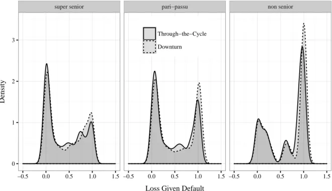
rates and realized LGDs on aggregated data. Observable macroeconomic and industry- specific information can be included as covariates in standard regression models to account for systematic risk (e.g., Chava and Jarrow (2004), Acharya et al. (2007) and Bellotti and Crook (2012)). Duffie et al. (2009) and Lando and Nielsen (2010) find evidence for addi- tional unobservable systematic effects in default risk which substantially increase credit risk in economic downturns. The dependency between default rates and LGDs is caused by observable systematic factors such as macroeconomic covariates (Chava et al. (2011)) and unobservable systematic factors that can be modeled by random effects (Bruche and González-Aguado (2010), Bade et al. (2011), Bellotti and Crook (2012) and Rösch and Scheule (2014)). The Basel Committee on Banking Supervision (2005) requires that LGD estimates shall reflect economic downturn conditions for regulatory purposes and account for the positive co-movement of PDs and LGDs. This is currently emphasized by the Eu- ropean Banking Authority (2017) which also advises to account for the bimodality of losses, i.e., the high number of total losses and recoveries.
Besides the question whether a borrower or debt instrument defaults, the literature also deals with the time in default. For instance, Bandopadhyaya (1994), Helwege (1999), Bris et al. (2006) and Denis and Rodgers (2007) study the time in bankruptcy and its determinants. Dermine and Neto de Carvalho (2006) and Gürtler and Hibbeln (2013) mention that the length of workout processes is empirically positively correlated with LGDs, i.e., the longer a debt is in default the more severe the loss is. The consideration of workout processes goes beyond the realized loss and provides additional information on the emergence of losses. Betz et al. (2016) find increased LGDs for long workout processes and time-varying levels in the length of defaults which indicates systematic effects in workout processes and workout LGDs.
Another field of study examines whether and to what extent bank capital requirements
burden institutions, particularly in recessions. Although the Basel Accords are intended
to prevent procyclicality, Gordy and Howells (2006) and Repullo and Suarez (2013) show
that regulatory capital requirements increase in recessions. In addition to regulatory
capital, institutions are obliged to hold loan loss provisions which are identified to increase
during recessions due to the underlying incurred loss model (Laeven and Majnoni (2003), Bikker and Metzemakers (2005) and Fonseca and González (2008)). The revised loan loss provisioning of the International Accounting Standards Board (2014) and the Financial Accounting Standards Board (2016) is based on an expected loss model and is intended to reduce procyclical effects and increase transparency of provisioning. However, the European Banking Authority (2016a) and the Basel Committee on Banking Supervision (2017) propose a transition period to provide institutions sufficient time to raise capital.
The Basel Committee on Banking Supervision (2016b) additionally points to the volatility of provisions due to the new standards.
Contribution
This thesis contributes to the literature on credit risk modeling and focuses on co- movements of risk parameters that intensify losses during recessions. The models provide more precise estimates of credit risk and a better understanding of systematic risk. This can improve risk-based capital reserves and can help to avoid a severe underestimation of risk and capital shortfalls in economic downturn periods. Furthermore, the discussion of regulatory requirements and the supervision of internal risk models can benefit from empirical results.
The literature and current discussions show that a closer look on the impact of eco-
nomic downturns on LGDs is still necessary. At the same time, the bimodality of losses,
i.e., the high number of total losses and recoveries, must be recognized. Although the
literature mentions a positive dependency between the length of workout processes and
LGDs, its significance and the role of systematic effects have not been analyzed. Further-
more, the revised loan loss provisioning will be based on lifetime expected losses and raises
the following questions amongst others. First, the sample selection of loss data causes
a positive dependency between single-period default risk and loss severity and must be
examined with respect to the maturity of financial instruments, i.e., a multi-period mod-
eling is necessary. Second, the impact of the new accounting standards on bank capital
requirements that are given by loan loss provisioning and regulatory frameworks must be
analyzed. This covers differences between both approaches of expected losses and how market participants and regulatory authorities may react. The research questions of the four following studies can be summarized as:
• How can the bimodality of losses, i.e., the high number of total losses and recoveries, adequately be modeled? Do covariate effects vary over the probability distribution of LGDs and, in particular, does the impact of economic downturns depend on quantiles as well as firm- and instrument-specific information?
• Are there systematic co-movements in the length of workout processes? How can the dependency be explained and to what extent does it affect credit risk (i.e., workout LGDs) and liquidity risk (i.e., the reduction of non-performing loans)?
• How does the positive dependency between default risk and loss severity evolve over multiple periods? What conclusions are necessary for the modeling and estimation of lifetime expected loss which is required by revised loan loss provisioning?
• What are the differences and similarities in the model requirements of the revised loan loss provisioning and the regulatory framework with respect to expected losses?
What is the impact of the new accounting standards on bank capital requirements?
The research questions are examined by advanced statistical methods. First, the
scope of LGD modeling is extended by proposing the quantile regression to separately
regress each quantile of the distribution. This approach enables a new look on covariate
and particularly downturn effects that vary over quantiles. Second, the length of workout
processes is a time variable and thus modeled by a Cox proportional hazards model, which
is similar to existing approaches on default times. Systematic effects are examined by the
inclusion of time-varying frailties. Third, lifetime expected losses are modeled by a copula
approach that combines accelerated failure time models for the default time with a beta
regression of the LGD. The use of copulas provide continuous-time LGD forecasts and
flexible dependence structures between default risk and loss severity. The fourth approach
combines a Probit model for the PD and a fractional response model for the LGD to
demonstrate the impact of revised loan loss provisioning on bank capital requirements.
In addition, goodness-of-fit measures enable to validate these approaches. Simulation studies and analyses of representative portfolios provide implications and demonstrate the significance of empirical results.
The use of comprehensive data strengthens the validity of empirical results. The first two studies use unique loss data from several banks on defaulted corporate loans with jurisdiction in the United States, Great Britain and Canada. The database provides workout LGDs and information on workout processes between 2000 and 2013, i.e., post- default cash-flows including repayments and costs. The other two studies use information on US American corporate bonds that provides defaults and market-based LGDs between 1982 and 2014. Both databases contain comprehensive covariate information with respect to the underlying instruments, borrowers and macroeconomic conditions.
This thesis presents four studies which separately examine the proposed research questions in Chapters 2 to 5. The remaining part of the introduction summarizes each study with respect to motivation, data, statistical method and contribution. Chapter 6 presents a conclusion and provides findings, a discussion and an outlook.
Chapter 2: Downturn LGD Modeling using Quantile Regression
The aim of capital reserves to reduce the risk of capital shortfalls is particularly pro-
nounced in recessions. The internal ratings-based approach of Basel II, therefore, re-
quires LGD estimates that reflect economic downturn conditions. The study contributes
to the literature by analyzing covariate and downturn effects on the entire bimodal shape
of losses that is characterized by the high number of total losses and recoveries. The
quantile regression of Koenker and Bassett (1978) and Koenker (2005) is used to sepa-
rately model each quantile of the distribution and to allow for quantile-specific effects of
covariates. The study is based on US American data of workout loan LGDs of small and
medium enterprises with defaults between 2000 and 2013. LGD estimates are evaluated
by goodness-of-fit measures that evaluate the entire distributional fit. The validation re-
veals advantages of quantile regression in comparison with standard regression techniques.
The analysis of quantile-varying covariate effects shows that the bimodality of losses can only partly be explained by firm- and loan-specific information as well as macroeconomic conditions. The paper concludes with a discussion on the impact of economic downturns on the distribution of loss rates and shows implications for the determination of downturn LGDs for regulatory purposes.
Chapter 3: Macroeconomic Effects and Frailties in the Resolution of Non-Performing Loans
The workout LGD of defaulted debt is determined by incoming cash flows and direct as well as indirect costs after default. The literature indicates that delayed workout pro- cesses are empirically correlated with higher losses. The study analyzes determinants of the length of workout processes and its significance for credit and liquidity risk of finan- cial institutions. The time from default to resolution of defaulted debt is modeled by a Cox proportional hazards model with stochastic time-varying frailties. This approach is comparable to Duffie et al. (2009) who investigate the time to default of US American bonds. The study uses data of defaulted loans from small and medium enterprises and large corporates with jurisdiction in the United States, Great Britain and Canada with defaults between 2004 and 2013. Besides firm- and loan-specific information, the anal- ysis discusses the role of observable (e.g., macroeconomic covariates) and unobservable (frailties) systematic factors. The latter are empirically identified to cause a significant co-movement of workout periods. In addition to a descriptive analysis of the correla- tion between resolution times and loss severity, a simulation study shows that economic downturns delay workout processes and thereby increase single-loan LGDs and portfo- lio losses. Furthermore, a second simulation study demonstrates that systematic effects between workout processes increase stable funding needs.
Chapter 4: A Copula Sample Selection Model for Predicting Multi-Year LGDs and Life- time Expected Losses
The revised loan loss provisioning will be based on lifetime expected losses and raises the
question how the positive co-movement of default risk and loss severity for the 12-month horizon behaves over the lifetime of financial instruments. The study develops a copula- based approach that enables a simultaneous modeling of default risk and loss severity for arbitrary time horizons. The rationale behind this is to combine regression models for the default time and the LGD by flexible dependence structures. The empirical work is done on US American corporate bond data for the years between 1982 and 2014. It controls for firm- and bond-specific as well as macroeconomic covariates. Several accelerated failure time models are examined to regress default times as in Lee and Urrutia (1996), Das et al.
(2007) and Orth (2013). The LGD is modeled by beta regression which is motivated by Gupton (2005) and Huang and Oosterlee (2012). The analysis reveals that the positive dependency of PDs and LGDs cause a decreasing term structure of loss severity, i.e., the longer a bond survives the lower the expected LGD is. The use of several copulas also demonstrates that correlation measures are not able to adequately capture the identified dependence structure. Finally, the empirical results indicate that standard credit risk models generally underestimate lifetime expected losses.
Chapter 5: The Impact of Loan Loss Provisioning on Bank Capital Requirements
The replacement of the incurred loss model for loan loss provisioning by an expected loss approach provides a convergence to the regulatory approach. The study discusses the new standards and remaining differences between expected losses for accounting and regulatory purposes with respect to the rating philosophy (through-the-cycle vs. point- in-time) and the required time period of possible losses (12-month vs. lifetime expected losses). Standard regression techniques are used to estimate the risk parameters PD and LGD, i.e., the Probit model (cf. Puri et al. (2017)) and a fractional response model (cf. Chava et al. (2011)). The study uses data of US American corporate bonds that were originated between 1991 and 2013. Expected losses for regulatory and accounting purposes are estimated and provisions as well as capital requirements are computed for stylized portfolios that are motivated by Gordy (2000) and Gordy and Howells (2006).
The study reveals a procyclical impact of the new accounting standards on regulatory
capital requirements. The impact is analyzed for different portfolio qualities, reinvestment strategies and states in the economic cycle. In addition, the criterion of a significant increase in default risk that determines the classification of instruments and its role for the transparency of provisioning is discussed.
Chapters 2 to 5 consist of independent studies with varying sets of co-authors. The first
study is published as an article in a peer-reviewed academic journal. The remaining three
studies are under review at the submission date of this thesis. Since the thesis consists of
independent studies submitted to journals with different style requirements, minor formal
differences exist across the chapters.
Downturn LGD Modeling using Quantile Regression
This chapter is joint work with Daniel Rösch
1and published as:
Krüger, S., Rösch, D. (2017). Downturn LGD modeling using quantile regression.
Journal of Banking & Finance 79, 42–56. DOI: 10.1016/j.jbankfin.2017.03.001
Abstract: Literature on Losses Given Default (LGD) usually focuses on mean pre- dictions, even though losses are extremely skewed and bimodal. This paper proposes a Quantile Regression (QR) approach to get a comprehensive view on the entire probability distribution of losses. The method allows new insights on covariate effects over the whole LGD spectrum. In particular, middle quantiles are explainable by observable covariates while tail events, e.g., extremely high LGDs, seem to be rather driven by unobservable random events. A comparison of the QR approach with several alternatives from recent literature reveals advantages when evaluating downturn and unexpected credit losses. In addition, we identify limitations of classical mean prediction comparisons and propose alternative goodness of fit measures for the validation of forecasts for the entire LGD distribution.
JEL classification: C51; G20; G28
Keywords: downturn; loss given default; quantile regression; recovery; validation
1
Chair of Statistics and Risk Management, Faculty of Business, Economics, and Business Information
Systems, University of Regensburg, 93040 Regensburg, Germany. E-Mail: daniel.roesch@ur.de
2.1 Introduction
2.1.1 Motivation and Literature
Practitioners and academics have investigated several statistical models for the measure- ment and management of credit risk. Initially, the focus was on the probability of default, whereas in recent years more attention was given to the loss in case of default. In addition, financial institutions need to evaluate their risk exposures for regulatory capital require- ments. Basel II introduced the internal ratings-based approach which enables institutions to provide their own estimates for the Loss Rate Given Default (LGD). However, because realized losses show a strong variation, particularly in recessions, the Basel Committee on Banking Supervision (2005) points to the importance of adequate estimates for economic downturns and unexpected losses. Thus, recent literature has started to extend the focus on expected LGDs to modeling an entire LGD distribution, but then usually aggregates the results to predictions of the mean.
Probably the most convenient LGD models use Ordinary Least Squares (OLS) (e.g., Qi and Zhao (2011)). Due to the non-normality of data, Dermine and Neto de Carvalho (2006) point to the need of data transformation and take into account the property of rates being between zero and one. An alternative to capture the shape of random variables which are ratios is presented by Gupton and Stein (2005) which assume a beta distribution for losses. Regression Trees are a non-parametric regression technique which splits the sample into groups and uses the groups’ means as estimates (e.g., Bastos (2010)). With respect to Downturn LGDs, Altman and Kalotay (2014) and Calabrese (2014) propose methods to decompose losses into possible components for different stages of the economic cycle. While the latter models take into account some aspects of Downturn LGDs, they usually do not model the entire distribution of LGD and do not provide determinants over the entire spectrum of LGDs.
An approach which is able to model the impact of covariates for LGDs over the
entire distribution is Quantile Regression (QR). Somers and Whittaker (2007) use QR
to model the asymmetric distributed ratio of house sale recoveries to indexed values and estimate mean LGDs of secured mortgages by aggregating these results. Siao et al.
(2015) apply QR to directly predict mean workout recoveries of bonds and show an improved performance compared to several methods by evaluating mean predictions.
The present paper extends these approaches by (1) studying a unique and comprehensive loan database of small and medium enterprises, (2) using Quantile Regression results for risk measures in a direct way without aggregating the distributions to mean predictions, and (3) extending the validation of mean predictions to evaluating the entire distribution of losses. This enables us to consider different parts of economic cycles and to provide an alternative approach for Downturn LGDs and unexpected losses.
Generally, the definition of Loss Rates Given Default differs depending on the kind of financial instrument. Market-based LGDs are given by one minus the ratio of bond prices after default and the instrument’s par value. It is the loss due to the immediate drop of bond prices after default and represents market beliefs of future recoveries. Jankowitsch et al. (2014) investigate determinants of market-based LGDs for US corporate bonds.
Their data are almost evenly distributed due to the weighting of extreme low and high final recoveries by mean expectations. In contrast, ultimate or workout LGDs reflect the finally realized payoff depending on the entire resolution process of the instrument and all corresponding cash flows and costs after default. Altman and Kalotay (2014) exhibit the high number of total losses and recoveries for workout processes of defaulted bonds and the difficulties of an adequate statistical modeling. Yashkir and Yashkir (2013) show that loan LGDs are bimodal, i.e., U-shaped for personal loans in the United Kingdom.
Dermine and Neto de Carvalho (2006) as well as Bastos (2010) identify similar properties for Portuguese loans of small and medium entities.
Some risk factors cause contrasting recoveries and LGDs during the workout process.
Examples are the nature of default, the type of resolution, the recovery of collateral, the macroeconomic conditions during resolution and also the length of the resolution process.
The prediction of these variables is a difficult task and, thus, U-shaped loss distributions
result prior to default. In addition, administrative, legal and liquidation expenses or
financial penalties (fees and commissions) and high collateral recoveries cause a significant number of LGDs lower than zero or higher than one. Most of the above-mentioned approaches are not able to capture both properties. Therefore, we suggest Quantile Regression which is suited to model extremely distorted distributions with bimodal shape without specific distributional assumptions or value restrictions of realizations.
This paper contributes to the literature in the following ways. First, our approach models the entire distribution of LGDs by Quantile Regression rather than predicting mean values. Thus, adequate measures for downturn scenarios and unexpected losses result can easily be derived. Second, this approach gives new insights into the impact of covariates over the entire spectrum of LGDs. For bimodal loan loss data, we distinguish between influences on extreme low, median and extreme high LGDs. Third, we pro- pose several validation approaches to compare our model to most common and capable methods by an in-sample and out-of-sample analysis.
Following this introductory remarks, we motivate the relevance of adequate distribu- tional estimates by an example. Section 2.2 contains a description of the QR approach and reference models. A simulation study explains theoretical advantages of the proposed method. Section 2.3 introduces the data and shows descriptive statistics. In Section 2.4, we show the model results and compare in-sample as well as out-of-sample performances of all models by different validation approaches. Afterwards, we show practical implica- tions in Section 2.5 and propose downturn measures. Section 2.6 summarizes the results.
2.1.2 Introductory Example
Most academic and practical credit risk models focus on mean LGD predictions (cf.
above mentioned literature). In addition, the Board of Governors of the Federal Reserve System (2006) proposes the computation of Downturn LGD measures by a linear trans- formation of means. This introductory example shows potential misleading results and interpretations.
Consider two loans with different stylized LGD distributions with the same mean.
Let the loss of loan 1 be uniformly distributed between zero and one and the LGD of
loan 2 be beta distributed with mean = 0.5 and variance = 0.125. Figure 2.1 shows the probability density functions. The means are equal, but the shapes differ. The LGD of loan 2 (dashed line) has more mass in the tails, particularly the probability of extreme losses is higher. Therefore, unexpected downturns may have a greater impact on loan losses compared to loan 1 (solid line). The concept of the Board of Governors of the Federal Reserve System (2006) does not account for this behavior and postulates the same downturn risk for both loans. The corresponding Downturn LGDs are given by 0.08 + 0.92 · E(LGD) = 0.54.
Figure 2.1: Stylized LGD Distributions
0 1 2 3
0.00 0.25 0.50 0.75 1.00
Loss Given Default
Density
Loan 1 Loan 2
Notes: The figure shows two stylized LGD distributions with same means and, thus, same Downturn LGDs proposed by the Board of Governors of the Federal Reserve System (2006). However, real quantiles and downturn as well as unexpected risk differ.
This paper proposes an alternative approach of downturn considerations by using
specific quantiles of the distribution, i.e., the Value at Risk (VaR). Thus, unexpected
downturn effects are modeled more accurately. For example, the 75 % - VaR for loan 1
is 0.75 due to uniformity. Loan 2 has a 75% - VaR of 0.85 and therefore higher risk for
this unexpected downturn. In this example, differences are found for all quantiles above
the 50 % - level and, thus, for potential downturn risk (see Table 2.1). This shows the
importance of adequate LGD models for regulatory purposes and the practical assessment
of credit risk by considering the entire spectrum of the LGD distribution and not the mean
only. This can easily be achieved by Quantile Regression which we briefly describe in the
next section.
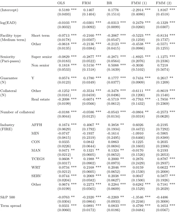
Table 2.1: Exemplary Downturn Loss Rates Given Default
DLGD Value at Risk
(FED) 50 % 75 % 90 % 95 % Loan 1: LGD in % 54.00 50.00 75.00 90.00 95.00 Loan 2: LGD in % 54.00 50.00 85.36 97.55 99.38
∆LGD in % 0.00 0.00 13.81 8.39 4.62
Notes: The table shows several LGD quantiles for two exemplary loans of Figure 2.1. Both dis- tributions have the same mean and, thus, the same Downturn LGD proposed by the Board of Governors of the Federal Reserve System (2006): 0.08 + 0.92 · E(LGD) = 0.54. However, the first loan has a uniform distributed LGD, whereas the second follows a beta distribution. This results in different Values at Risk.
2.2 Modeling Loss Given Default
2.2.1 Quantile Regression
Standard regressions, e.g., the method of ordinary least squares, model the mean and do not adequately consider the entire distributional nature. They usually fail making adequate VaR forecasts when the LGD distribution is, for instance, bimodal. A useful alternative is Quantile Regression (QR) proposed by Koenker and Bassett (1978) and Koenker (2005). For Y = LGD the VaR to a certain level τ ∈ (0, 1) is the (unconditional) τ -quantile
Q
Y(τ ) = inf {y ∈ R |F
Y(y) ≥ τ}, (2.1)
which is the maximum loss that is exceeded in at least (1 − τ ) · 100 % of all cases. QR allows modeling each quantile individually by separate regressions. Suppose we want to model the (conditional) τ-quantile given some control variables, the regression equation is
Y
i= β(τ )
0x
i+ ε
iτ(2.2)
with loans i = 1, . . . , n and x
ias covariate vector including a one for the intercept and β(τ) as unknown parameter vector. With Q
τ(ε
iτ) = 0, we have the τ -quantile of the LGD given by Q
τ(Y
i) = β(τ )
0x
i. There is no need to make any more model assumption for the errors ε
iτexcept of uncorrelatedness. Thus, non-normal, skewed and bimodal behaviors of LGDs can easily be handled. Hence, we allow for a high level of error heterogeneity. The unknown parameter vector is estimated by minimizing the following objective function over β(τ ):
n
X
i=1
ρ
τ(y
i− β(τ )
0x
i) with ρ
τ(x) =
τ x , if x ≥ 0, (1 − τ )|x| , else.
(2.3)
Equation (2.3) shows the minimization of weighted residuals by the asymmetric loss function ρ
τ. In contrast, the method of Ordinary Least Squares uses a quadratic loss function to model the mean. Here, for the right tail of the distribution positive residuals are stronger weighted by τ ∈ (0.5, 1) than negative residuals by 1 − τ . This leads to the regression of the τ -th quantile with an unbiased, consistent and asymptotically normally distributed estimator.
2.2.2 Simulation Study
In contrast to standard regression techniques, Quantile Regression is able to capture several statistical issues that may cause non-normality. To illustrate this property, we consider two exemplary simple linear models with different reasons for bimodality. Given the data generating processes of Table 2.2, we simulate two datasets and identify serious issues when estimating the linear models with OLS and show the capability of Quantile Regression. For each model, a normally distributed covariate x is connected over a linear function with an intercept β
1, slope β
2and an error term u.
The first model is given by an intercept of β
1= 0.5, a slope of β
2= 1 and a bimodal
error that is generated by the sum of a Gaussian and a Bernoulli distribution. The second
model uses a normally distributed error but assumes varying values for the intercept and
Table 2.2: Simulation – Data generation
Bimodal errors Binomial parameters Model y
i= β
1+ β
2x
i+ u
iy
i= β
1τi+ β
2τix
i+ u
iCovariate x
ias sample of X ∼ N (0, 0.01) Parameters β
1= 0.5 β
1τi= z
τiβ
2= 1 β
2τi= z
τi− 0.5 Z
τi∼ B(0.5) Error term U
i= V
i+ W
iU
i∼ N(0, 0.04)
V
i∼ N (0, 0.04) W
i∼ B(0.5)
Notes: We simulate bimodal data with the models shown here. All random variables are gener- ated independently. Afterwards, we estimate both models with OLS and Quantile Regression.
the slope. Lower conditional quantiles, i.e., given the covariate information, are generated with β
1= 0 and β
2= −0.5. In contrast, upper conditional quantiles are calculated with β
1= 1 and β
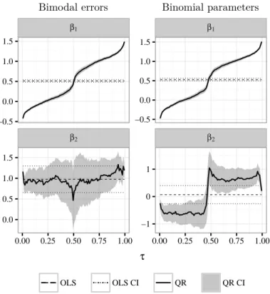
2= 0.5. A Bernoulli distribution determines independently for each individual whether a lower or upper quantile is generated. We refer to both models as ‘bimodal errors’ and ‘binomial parameters’ model and independently simulate 1,000 observations each. Figure 2.2 shows the resulting bimodal distribution of the generated data.
Figure 2.2: Simulation – Data generation
Bimodal errors Binomial parameters
0 25 50 75 100
−1 0 1 2 −1 0 1 2
y
Frequenc y
Notes: The figure shows simulated observations for both linear models of Table 2.2. The left panel is generated by bimodal errors, whereas in the right panel parameters vary over quantiles.
After generating bimodal data, we estimate linear models for the dependent variable
y with an intercept β
1, the covariate x and the corresponding slope β
2. From this point
of view, i.e., for estimation, the source of bimodality is unknown for both datasets.
Figure 2.3 shows parameter estimates for OLS and Quantile Regression. For the model with bimodal errors, which is shown on the left panel, OLS leads to plausible and constant parameter estimates. QR shows varying intercepts for different quantiles, because it aggregates the information of a regression constant and a bimodal error term. Overall, the slope is reliably estimated by QR. For the second model with normally distributed errors but binomial parameters, OLS is unable to capture non-constant parameters. This leads to distorted estimates of the intercept and the slope. The latter parameter is not even statistically significant different from zero, i.e., OLS does not capture the significant role of the covariate. In contrast, Quantile Regression is able to capture the differences in lower and upper quantiles. The intercept contains the two distinct values for the level as well as the normally distributed error. The slope is identified as a statistically significant covariate with varying influence.
Figure 2.3: Simulation – Parameter estimation
Bimodal errors Binomial parameters
β1β2
β1
β2
−0.5 0.0 0.5 1.0 1.5
0.0 0.5 1.0 1.5
−0.5 0.0 0.5 1.0 1.5
−1 0 1
0.00 0.25 0.50 0.75 1.00 0.00 0.25 0.50 0.75 1.00
τ
OLS OLS CI QR QR CI
Notes: The figure shows parameter estimates for the data shown in Figure 2.2 and generated by the
models of Table 2.2. The left panel contains estimates for the model with a bimodal error term, whereas
the right panel presents results for the model with binomial parameters. The confidence intervals (CI)
are shown for the 95 % - level and are calculated for Quantile Regression with standard errors that are
estimated by kernel estimates.
For both data generating processes, Figure 2.4 shows 1,000 independently simulated observations each using OLS and QR parameter estimates of Figure 2.3. Neither the bimodal error nor the binomial parameters are captured by OLS due to the assumptions of normally distributed errors and constant parameters. Thus, only QR is able to capture the bimodality of the data generating processes.
Figure 2.4: Simulation – Forecasting
Bimodal errors Binomial parameters
0 50 100 150
−1 0 1 2 −1 0 1 2
y
Frequenc y
OLS QR
Notes: The figure shows simulated data using the parameter estimates of Figure 2.3. The bimodality of the data generating process is only captured by Quantile Regression.
2.2.3 Comparative Methods
This paper compares QR to the most popular LGD models. We use the OLS method as the first benchmark model as proposed in Qi and Zhao (2011) and calculate quantiles by fitting a normal distribution for estimated errors. Secondly, a Fractional Response Model (FRM) is used which transforms the dependent variable before doing an OLS to bring it closer to normality (cf. Dermine and Neto de Carvalho (2006)). Here, we use the inverse normal regression by transforming the LGD with the inverse cumulative density function of the normal distribution as proposed by Hu and Perraudin (2002).
2The FRM and most LGD models assume the dependent variable to be a rate, i.e., to be bounded by zero and one. Here, we have data with plausible values out of this range, which is also relevant for creditors. Reasons are administrative, legal and liquidation expenses or financial penalties (fees and commissions) and high collateral recoveries. In
2
We tested several transformation, but only present the best performing alternative, i.e., the inverse
normal regression.
order to apply the FRM and other models for comparative reasons, we transform the observed LGD to lie in this interval for these models.
3In addition, we add an adjustment parameter of 10
−9to avoid values on the bounds as proposed by Altman and Kalotay (2014). After estimation we re-transform predicted values to the observed LGD scale.
Gupton and Stein (2005) propose Beta Regression (BR) which is our third benchmark model.
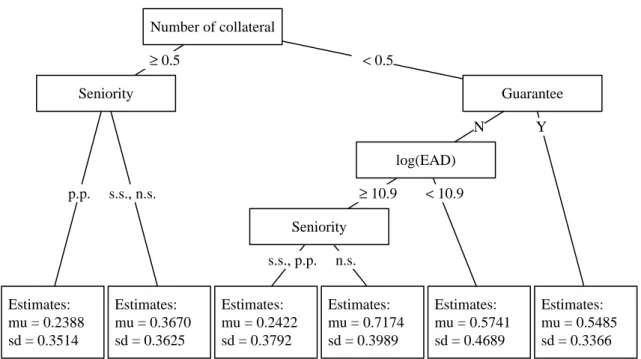
The fourth model is Regression Trees (RT) which are a non-parametric regression technique, which splits data into groups and uses the groups’ averages of the dependent variable as their mean prediction (see Bastos (2010)). Similar to OLS, we fit normal distributions per group for quantile predictions.
Table 2.3: Comparative methods
Method Exemplary literature
Ordinary Least Squares Qi and Zhao (2011),
(OLS) Loterman et al. (2012)
Fractional Response Model Bastos (2010),
(FRM) Chava et al. (2011),
Qi and Zhao (2011), Altman and Kalotay (2014) Beta Regression Huang and Oosterlee (2012),
(BR) Loterman et al. (2012),
Yashkir and Yashkir (2013) Regression Tree Bastos (2010),
(RT) Qi and Zhao (2011),
Loterman et al. (2012), Altman and Kalotay (2014) Finite Mixture Model Calabrese and Zenga (2010),
(FMM) Loterman et al. (2012),
Altman and Kalotay (2014) Notes: We compare the performance of each of the five models with Quantile Regression.
Finally we apply Multistage Models which estimate probabilities of low, middle or high LGDs. Afterwards, the distribution of each component is modeled (see Altman and Kalotay (2014)). Some of these methods directly model probabilities of obtaining values of exactly zero or one and do not allow for values outside these bounds. Thus, these models are not able to cover the kind of bank loan LGDs that we observe, i.e., with several observations lower than zero and higher than one. In contrast, a Finite
3
The transformation is done by LGD
[0,1]=
LGD−min(LGD) max(LGD)−min(LGD).
Mixture Model (FMM) assumes a mixed distribution of several margins. This paper uses a normal mixture distribution for the LGD.
4Quantiles are directly observed from mixture distributions. Table 2.3 shows a summary of comparative methods from the literature.
2.3 Data
This paper uses a dataset of US American defaulted loans of small and medium enter- prises from Global Credit Data (GCD) which provides the world largest LGD database.
The association consists of 52 member banks from all over the world including global systemically important banks. Members exchange default data to develop and validate their credit risk models. We restrict the sample to all defaults since year 2000 to ensure the consistent default definition of Basel II. Since workout processes of recent defaults are not necessarily completed, we do not account for defaults after 2013. Cures are not considered because they do not provide default data with actual losses. We remove loans with exposures at default of less than 500 US $ because of minor relevance and to satisfy a materiality threshold.
Since we use loan data, we consider workout Recovery Rates (RR) including post- default cash flows. The RR is the difference of all discounted incoming cash flows (CF
+) and discounted direct as well as indirect costs (CF
−), divided by the exposure at default (EAD). The LGD is given as one minus the RR:
LGD = 1 −
P CF
+− P CF
−EAD . (2.4)
Incoming cash flows (CF
+) are: principal, interest and post-resolution payments, the recorded book value of collateral, received fees and commissions, and waivers. Direct and indirect costs (CF
−) are: legal expenses, administrator and receiver fees, liquidation expenses, and other workout costs. In addition to the exposure at default, the nominator
4
In contrast to Altman and Kalotay (2014), we do not transform the dependent variable because we
observe values out of the interval between zero and one. Actually, a transformation would lower the
goodness of fit for mixture models for our dataset. Thus, we use raw data to allow a fair comparison. In
addition, we tested a beta mixture distribution, which we do not report because of a worse performance
compared to the normal mixture model.
of Equation (2.4) contains discounted principal advance, financial claim, interest accrual, and fees and commissions charged. All numbers are discounted by LIBOR to the default date.
We use two selection criteria due to Höcht and Zagst (2010), Höcht et al. (2011) and Betz et al. (2016) to ensure consistent as well as plausible data and to detect outliers.
First, we consider loans for which the sum of all cash flows and further transactions, e.g, charge-offs, are between 90 % and 110 % of the outstanding exposure at default. Second, we regard loans with payments between -10 % and 110 % of the outstanding exposure at resolution. Actually, this selection procedure is less important for Quantile Regression because it is less sensitive to outliers. Nevertheless, we remove these loans as well as all observations with LGDs outside of [−0.1, 1.1] to allow a fair comparison to standard regression techniques which are typically more sensitive to outliers.
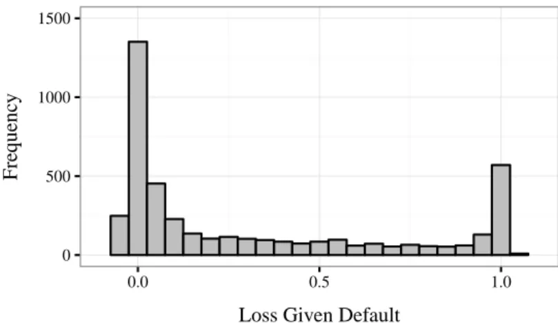
Figure 2.5 shows a histogram of the final dataset. Most LGDs are nearly total losses or total recoveries which yields to a strong bimodality. The mean is given by 0.31 and the median by 0.09, i.e., LGDs are highly skewed. Both properties of the distribution may favor the application of QR because most standard methods do not adequately capture bimodality and skewness. Furthermore, many LGDs are lower than 0 and higher than 1 due to administrative, legal and liquidation expenses or financial penalties (fees and commissions) and high collateral recoveries.
Figure 2.5: Observed Loss Rates Given Default
0 500 1000 1500
0.0 0.5 1.0
Loss Given Default
Frequenc y
Notes: LGD calculation includes all cash flows and direct as well as indirect costs. All components are
discounted to the loan’s default date.
The yearly mean LGD and the distribution of default over time are visualized in Fig- ure 2.6. The number of observed defaults strongly increased during the Global Financial Crises and slowly decreased in the aftermath. Loss rates were high due to the recession in 2000 and 2001 and subsequently decreased. In the last crises, the loss severity returned to a high level, where it remains since then.
Figure 2.6: Loss Rates Given Default over time
0.0 0.1 0.2 0.3 0.4
2000 2005 2010
As ratio of 100%
Mean LGD
# defaults
Notes: The figure shows yearly mean LGDs and the ratio (number of defaults per year) / (total number of defaults).
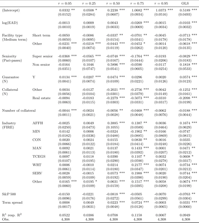
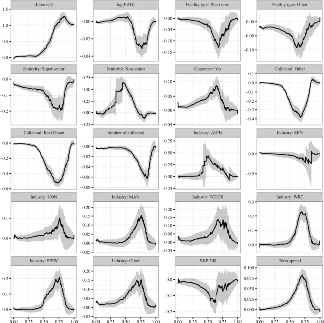
Table 2.4 shows descriptive statistics for the covariates of which we can make use in the database. For metric variables we report their means and several quantiles. For each level of categorical variables we show means and category-specific quantiles of the LGD as well as the number of observations per group. Medium term facilities imply higher LGDs than other facility types. For example, the median realized LGD for medium term facilities is 0.18 compared to 0.03 for short term facilities and 0.01 for other types. The seniority plays an important role for losses. On average non senior secured loans result in high LGDs of 0.64 compared to the super senior category with 0.30. We distinguish between loans with and without guarantees, i.e., whether there is an additional guarantor for a loan. In the mean, there is only a small difference for loans with or without guarantees. However, in the median we see a difference for loans with (0.16) and without (0.07) guarantees.
Although a guarantee should reduce future losses, it can provide asymmetric information
problems like moral hazard which can lead to higher losses. In addition, we distinguish
between loans without any collateral, with real estate and with other collateral. Loans
with real estate collateral produce lowest mean LGDs with 0.17 compared to 0.44 for loans without any collateral. The firms’ industry affiliations may determine the magnitude of losses. For most industries, the mean LGD is around 0.30 - 0.35. The maximum value is given by the group of agriculture, etc. (0.46) and the minimum is given by the mining industry (0.21). Financial affiliation results in low mean LGDs of 0.25.
Table 2.4: Descriptive statistics
Variable Level Quantiles Mean Obs.
0.05 0.25 0.50 0.75 0.95
LGD -2.99 0.32 9.01 61.56 100.00 31.27 4,308
log(EAD) 9.52 11.38 12.68 13.82 15.68 12.61 4,308
Facility type Medium term -0.90 2.40 17.52 67.46 100.00 35.58 2,372 Short term -1.30 0.87 3.28 51.87 100.00 26.57 559
Other -4.45 -1.02 1.31 49.74 100.00 25.76 1,377
Seniority code Pari-passu 2.60 6.92 17.84 65.41 102.32 35.77 713 Super senior -3.38 0.09 5.07 58.75 100.00 29.85 3,539 Non senior -0.17 16.38 91.02 100.75 100.79 63.64 56 Guarantee indicator N (no guarantee) -3.65 0.00 6.92 62.99 100.00 30.20 2,587 Y (guarantee) -0.73 1.53 15.79 60.48 100.00 32.88 1,721 Collateral indicator N (no collateral) -2.46 0.42 33.28 96.29 100.00 44.01 1,152
Other -2.24 0.72 8.02 54.76 100.00 29.33 2,464
Real estate -4.97 -0.58 1.56 22.97 95.97 16.99 692
Number of collateral 0.00 0.00 1.00 1.00 4.00 1.32 4,308
Industry
Finance, insurance, real estate (FIRE) -4.10 -0.29 5.96 43.87 100.00 25.38 646 Agriculture, foresty, fishing, hunting (AFFH) -3.80 -0.14 61.04 84.96 100.33 46.43 36
Mining (MIN) -0.42 0.71 2.06 20.83 98.94 21.43 21
Construction (CON) -3.87 -0.52 8.51 56.53 100.00 29.23 459
Manufacturing (MAN) -2.71 0.12 4.96 68.33 100.00 31.55 639
Transp., commu., elec., gas, sani. serv. (TCEGS) -1.33 0.36 22.13 59.72 100.00 34.62 173
Wholesale and retail trade (WRT) -3.41 0.05 4.55 62.60 100.00 30.93 590
Services (SERV) -3.77 0.13 5.42 81.29 100.00 33.76 704
Other (Other) 0.66 3.93 14.71 59.90 101.53 33.29 1,040
S&P 500(rel. change) -0.28 0.01 0.11 0.18 0.33 0.08 4,308
TED spread(abs. spread in p. p.) 0.13 0.19 0.26 0.46 1.32 0.44 4,308 Term spread(abs. spread in p. p.) 0.07 1.94 2.63 3.28 3.50 2.40 4,308
VIX(abs. in p. p.) 12.70 16.52 18.00 25.61 42.96 21.90 4,308
Notes: The table shows means and quantiles of empirical LGDs for categorical variables with corresponding numbers of observation. In addition, the means and quantiles of metric variables, i.e., LGD, log(EAD) and number of collateral are given.
We also use two macroeconomic control variables. For the overall real and financial
environment, we use the relative year-on-year growth of the S&P 500. Stock exchange per-
formances are identified as general LGD drivers, e.g., by Qi and Zhao (2011) and Chava
et al. (2011). Both papers study bond data and identify the three-month treasury-bill
rate as a significant variable to consider expectations of future financial and monetary conditions. This paper uses loan data for which we find the absolute term spread between 10-years and 3-months US treasury rates to be significant drivers for LGDs which is also identified by Lando and Nielsen (2010) as a driver of credit losses in general. Macroeco- nomic information corresponds to each loan’s default year. Both variables result in most plausible and significant results when testing different lead and lag structures. We also tested other popular macroeconomic variables, e.g., inflation, the volatility index VIX, industry production, gross domestic product, interest rates and the TED spread, which result in less explanatory power.
52.4 Empirical Analysis
2.4.1 Quantile Regression
In this section the results of QR are provided. Table 2.5 shows the estimation results of QR for the 5th, 25th, 50th, 75th and 95th percentile and the corresponding OLS estimates. A full picture for all percentiles is given in the Appendix (Figure 2.A.1). As can be seen the level and significance of the parameter estimates strongly depend on the respective quantile.
The regression constant shows the behavior of the dependent variable when keeping covariates at zero. The course does not suggest normally distributed error terms, which would result in a smoothed s-shape. For low quantiles the intercept is near total recovery and starts to increase monotonically around the median until it reaches its maximum around total loss at higher quantiles. Loan losses generally exhibit a wide range regardless of control variables, which is due to the bimodal nature of LGDs. At the tails (5th and 95th percentile) most covariates are not statistically significant different from zero. This means that the extreme events, e.g., very high LGDs, are not explainable by our covariates and mainly due to unpredictable events.
5