Precision Spectroscopy of Positronium Using a Pulsed Slow Positron Beam

Research Collection

Doctoral Thesis

Precision Spectroscopy of Positronium Using a Pulsed Slow Positron Beam

Author(s):

Heiss, Michael Wolfgang Publication Date:

2021

Permanent Link:

https://doi.org/10.3929/ethz-b-000477081

Rights / License:

In Copyright - Non-Commercial Use Permitted

This page was generated automatically upon download from the ETH Zurich Research Collection. For more information please consult the Terms of use.

Diss. ETH No. 27501

Precision Spectroscopy of Positronium Using a Pulsed Slow Positron Beam

A thesis submitted to attain the degree of Doctor of Sciences

(Dr. sc. ETH Zurich)

presented by Michael Wolfgang Heiss

MSc ETH, ETH Zurich

born on 13

June, 1986 citizen of Austria

accepted on the recommendation of Prof. Dr. Paolo Crivelli , examiner Prof. Dr. Klaus Stefan Kirch , co-examiner

Prof. Dr. Anna Sótér , co-examiner Prof. Dr. Dylan Yost , co-examiner

2021

I. Abstract

Positronium is the lightest known atom and comprises a structureless point-like electron and its anti-particle, the positron. As such, it is purely leptonic and can be described to very high precision by bound-state QED without the inherent complications given by the finite size and quark substructure of protonic atoms. Furthermore, being a true onium atom, recoil effects are strongly enhanced and its quantum numbers sum to zero, making it an ideal candidate to test fundamental symmetries like CPT-invariance.

However, positronium is also a very challenging system for precision measurements due to its ephemeral nature. Being a bound state of anti-particles it tends to self- annihilate quickly and due to its lightness it exhibits much larger velocities than other atoms. Nevertheless, being a precision test-bench for QED with many unique features, it represents a particularly interesting system for spectroscopic measurements. This thesis presents the efforts towards precise determinations of the 1

S

→ 2

S

transition and both the hyperfine and fine structure of positronium in the n = 2 state.

The pulsed slow positron beamline at ETH Zurich, being a key prerequisite for these measurements, was optimized and a new beam transport and bunching system was developed. It was found that the efficiencies were comparable to similar beamlines and several further possible improvements were identified.

This thesis includes a measurement of the 1

S

→ 2

S

transition by Doppler-free two-photon laser spectroscopy of 1 233 607 210 . 5 MHz ± 49 . 6 MHz, which paves the way towards a new precision determination of this interval. Improvements by roughly two orders of magnitude on this result are suggested and discussed.

The design of an experiment to measure the hyperfine transition in the first excited state is presented. A microwave system supporting more than 100 kW of circulating power was developed and tested. Extensive simulations of the excitation and detection show the expected sensitivity to be 9 . 9 ppm (statistical) and 2 . 8 ppm (systematic) and further envisioned improvements are presented. This measurement will constitute the first measurement of this transition and the first determination of a hyperfine interval of positronium in vacuum altogether.

It was found that the experimental setup directly supports a determination of the

2

S

→ 2

P

interval. Minor changes allow also for the measurement of the 2

S

→

2

P

and 2

S

→ 2

P

transitions. Simulations show the expected sensitivities to be

approximately 7 ppm (statistical) and 0 . 5 ppm (systematic), which will allow to shed light

on a 4.5σ discrepancy of the most precise fine structure measurement in positronium with

theory calculations.

II. Zusammenfassung

Positronium ist das leichteste bekannte Atom und besteht aus dem strukturlosen punkt- förmigen Elektron und seinem Antiteilchen, dem Positron. Als solches ist es rein lepto- nisch und kann durch die Quantenelektrodynamik mit sehr hoher Präzision beschrieben werden, ohne die inhärenten Komplikationen, die durch die endliche Grösse und Quark- Substruktur protonischer Atome entstehen. Da es sich um ein echtes Onium-Atom han- delt, sind die Rückstosseffekte stark verstärkt und seine Quantenzahlen summieren sich zu Null. Dies macht es zu einem idealen Kandidaten, um fundamentale Symmetrien wie die CPT-Invarianz zu testen.

Positronium ist jedoch aufgrund seiner kurzlebigen Natur auch ein sehr herausfor- derndes System für Präzisionsmessungen. Da es sich um einen gebundenen Zustand von Antiteilchen handelt, neigt es dazu, innerhalb kürzester Zeit zu annihilieren und weist aufgrund seiner geringen Masse viel höhere Geschwindigkeiten auf als andere Atome.

Als Präzisions-Testumgebung für die Quantenelektrodynamik, mit vielen einzigartigen Merkmalen, stellt es dennoch ein besonders interessantes System für spektroskopische Messungen dar. In dieser Arbeit werden die Bemühungen um eine präzise Bestimmung des 1

S

→ 2

S

Übergangs sowie der Hyperfein- und Feinstruktur von Positronium im Zustand n = 2 vorgestellt.

Der gepulste langsame Positronenstrahl an der ETH Zürich, der eine wesentliche Vor- aussetzung für diese Messungen ist, wurde optimiert und ein neues Strahltransport- und Kompressionssystem wurde entwickelt. Es hat sich gezeigt, dass die Wirkungsgrade mit jenen von ähnlichen Aufbauten vergleichbar waren, und es wurden mehrere weitere mögliche Verbesserungen identifiziert und präsentiert.

Diese Arbeit beinhaltet eine Messung des 1

S

→ 2

S

Übergangs durch Doppler- freie Zwei-Photonen-Laserspektroskopie von 1 233 607 210, 5 MHz ± 49, 6 MHz, die den Weg für eine neue Präzisionsbestimmung dieses Intervalls ebnet. Verbesserungen dieses Ergebnisses um ungefähr zwei Grössenordnungen werden vorgeschlagen und diskutiert.

Der Aufbau eines Experiments zur Messung des Hyperfeinübergangs im ersten ange- regten Zustand wird vorgestellt, wofür ein Mikrowellensystem mit einer zirkulierenden Leistung von mehr als 100 kW entwickelt und getestet wurde. Umfangreiche Simulationen der Anregung und Detektion zeigen eine erwartete Sensitivität von 9, 9 ppm (statistisch) and 2 , 8 ppm (systematisch) und weitere geplante Verbesserungen werden vorgestellt.

Diese Messung würde die erste Messung dieses Übergangs und die erste Bestimmung eines Hyperfeinintervalls von Positronium im Vakuum überhaupt darstellen.

Es wurde festgestellt, dass der entwickelte Versuchsaufbau ebenso eine Bestimmung

des 2

S

→ 2

P

Intervalls unterstützt. Kleinere Änderungen ermöglichen ausserdem

die Messung der Übergänge 2

S

→ 2

P

und 2

S

→ 2

P

. Simulationen zeigen, dass

die erwarteten Sensitivitäten bei ungefähr 7 ppm (statistisch) and 0 , 5 ppm (systema-

tisch) liegen, was es ermöglichen wird, eine 4 , 5 σ -Diskrepanz der momentan genauesten

Feinstrukturmessung mit theoretischen Berechnungen zu überprüfen.

III. Acknowledgements

Whenever I near the conclusion of a momentous chapter of my life – which the pursuit of a PhD certainly is – I can’t help but look back and reminisce. Increasingly, I find that the most important part is not the final destination, but the journey. And what is a journey without great people to walk with and guide you along the path?

My sincere gratitude goes to Prof. Paolo Crivelli, who guided me in my professional career like no one else, always willing to share his immense knowledge and to help find solutions to problems which might have seemed insurmountable at first. I would like to express my appreciation for the encouragement and introduction provided by Prof.

Eberhard Widmann, without whom I might not have taken this particular direction. I would also like to thank Prof. André Rubbia for his supervision in the early phases and Prof. Klaus Kirch, Prof. Anna Sótér, and Prof. Dylan Yost for examining this thesis and thereby acting as gatekeepers for my destination.

I was truly fortunate to work with so many extremely talented people over the years.

Among them, Dr. Dave Cooke and Dr. Pauline Comini, who introduced me to the intricacies of the pulsed positron beamline and the pulsed dye amplifier. I also had the great pleasure to work with Dr. Carlos Vigo Hernandez and Dr. Lars Gerchow and enjoy their many insights into positron beams, MCPs and much more. My gratitude also goes out to Dr. Artem Golovizin for sharing his expertise of all things laser-related and for being the best guide of Moscow one could wish for. I would also like to thank Dr.

Balint Radics, Dr. Ben Ohayon and Dr. Zak Burkley for many enlightening discussions and help along the way.

A great pleasure and learning experience was the chance to supervise highly curious and talented Master students. Without a doubt many of them will go on to become great physicists. I would especially like to thank Lucas de Sousa Borges for his support in the late stages of the 1S-2S measurement and for taking up the torch of positronium spectroscopy at ETH.

What made life much more enjoyable, were the amazing colleagues at ETH: Mr. Dr.

Emilio Depero, Gianluca Janka, Alexander Stauffer, Johannes Wüthrich, Paul Prantl, Ibâa El-Maïs, Philipp Blumer, Dr. Laura Molina Boleno, Henri Sieber, Irene Cortinovis, Mark Rajmaakers, Benjamin Banto Oberhauser and so many more with whom I had great conversations about physics, life, and Rick and Morty – not necessarily in that order.

My deepest gratitude goes to my family, to my aunt Karin for sparking my curiosity in physics and to my parents Renate and Wolfgang for always supporting me in times of need. Without them, going on this adventure would not have been possible. Sadly, my mother did not live to see me reach this milestone, but I know she would be very proud.

Finally, and most importantly, I want to thank my wife Carina for her unwavering

love and support. Putting up with me and my quirks for more than a decade is surely

a bigger achievement than writing this thesis.

Contents

I. Abstract 1

II. Zusammenfassung 3

III. Acknowledgements 5

1. Introduction 9

1.1. Positronium: the fleeting atom . . . . 9

1.1.1. The history of the positron and positronium . . . . 9

1.1.2. Properties of positronium . . . 10

1.2. Precision test bench for QED . . . 12

1.2.1. The theory of the positronium atom . . . 13

1.2.2. The excited state lifetime . . . 17

1.2.3. The experimental history of positronium spectroscopy . . . 18

1.3. A window to the world beyond the Standard Model . . . 19

2. Pulsed slow positron beamline 21 2.1. Overview . . . 21

2.2. Positron source and moderation . . . 22

2.3. Buffer gas trap . . . 36

2.4. Pulsed beam transportation and implantation . . . 44

3. Laser spectroscopy of Positronium 55 3.1. Overview . . . 55

3.2. Positronium formation . . . 56

3.3. Laser Excitation . . . 63

3.3.1. 1S-2S excitation (486 nm) . . . 64

3.3.2. 2S delayed photo-ionization (532 nm) . . . 67

3.3.3. 2S-20P excitation (736 nm) . . . 68

3.3.4. Frequency stabilization and measurement . . . 71

3.4. Detection system . . . 72

3.5. Theoretical background and simulation . . . 81

3.5.1. Description of Monte Carlo simulation . . . 84

3.5.2. Simulation results . . . 89

3.6. Results of the 1S-2S pulsed excitation measurement . . . 96

4. Microwave spectroscopy of Positronium 107 4.1. Introduction . . . 107

4.2. Overview . . . 109

4.3. Laser Excitation . . . 111

4.4. Microwave Excitation . . . 113

4.4.1. Electromagnetic field configuration . . . 120

4.4.2. Further design considerations . . . 123

4.4.3. Experimental results on cavity performance: . . . 127

4.5. Detection system . . . 129

4.5.1. Hyperfine structure detection system . . . 129

4.5.2. Fine structure detection system . . . 134

4.6. Expected sensitivity . . . 135

4.6.1. Hyperfine structure measurement . . . 135

4.6.2. Fine Structure Measurement . . . 140

5. Conclusion and future prospects 144 5.1. Pulsed slow positron beamline . . . 144

5.2. Precision measurement of the 1S-2S transition . . . 145

5.3. Precision measurement of the 2S hyperfine and fine structure splittings . . 148

List of Figures 150

List of Tables 154

References 155

Appendix A. Schematic overview of the 1S-2S laser excitation system 170

Appendix B. Technical drawings of confocal mirrors 171

Appendix C. Schematics of time-buncher and elevator 174

1. Introduction

1.1. Positronium: the fleeting atom

1.1.1. The history of the positron and positronium

Paul Dirac postulated the famous Dirac equation in the quest to create a relativistic version of Quantum Mechanics in 1928 [1]. The importance of this work was immediately clear, since it finally allowed to successfully explain the origin of electron spin. Despite being a very compelling theory, it seemed to have one fatal flaw, namely the existence of negative energy solutions. This suggested the simultaneous existence of electrons with negative and positive charge and possibly even oscillations from one to the other.

It took Dirac three more years and multiple attempts to explain this peculiar feature by postulating that in fact the theory does not only describe electrons, but also another type of particle, which he called the anti-electron [2] – and hence, the idea of the positron was born. It did not even take a full year for Carl Anderson to discover [3] this anti- electron, or as he named it

– the positron – taking thousands of photographs using his Wilson cloud chamber (see figure 1).

The year following Andersons publication, Stjepan Mohorovičić postulated a bound state of electron and positron [5], which he initially called Electrum and suggested to look for it via astronomical spectroscopy. After this flurry of activity it would take more than a decade until Arthur Ruark proposed a spectroscopic measurement of this bound state [6] – which he called Positronium – using intense positron beams that have become available with the introduction of the betatron. He already noted the exceptional difficulty such a measurement posed due to the inherent properties of positronium, which we will discuss later in this section.

Finally, in 1951 Martin Deutsch experimentally showed the formation of long-lived positronium states in nitrogen gas [7] using a

Na source and PALS – Positron Annihi- lation Lifetime spectroscopy – a detection method he pioneered. This technique, which has been continuously developed and is still widely used, measures the time between a start signal relative to the formation of positronium and a signal compatible with either the annihilation of the positron or the decay of positronium. In the original experiment Deutsch took advantage of the fact that when

Na undergoes β

decay and emits a positron, the daughter isotope (

Ne

) decays to its ground state via the emission of a 1275 keV photon with a lifetime of only 3 . 7 ps. A scintillator was placed close to the source to detect this nuclear de-excitation photon and another scintillator, placed in a lead cylinder to shield from the source, was used to monitor the decay volume. Deutsch showed that the relatively high energy positrons could ionize the gas atoms and pick up an electron and thereby forming positronium. Three quarters of those atoms were formed in long-lived states (due to the respective spin states, see next section), which produced a delayed signal in the scintillator when they decayed. To make sure this delayed signal was indeed from positronium and not some unexpected background, he

1To be precise, it should be noted that the name positron was actually coined by Watson Davis, the editor in charge of Andersons publication in Science [4].

Figure 1: Discovery of the positron – the picture shows a photograph taken in Andersons cloud chamber of a 63 MeV positron, entering from the lower left, passing a 6 mm lead plate and emerging with approximately 23 MeV. From the direction and length of the curve one can see that this is indeed a positive particle, which is found to be significantly lighter than a proton. ( source: [3])

added a small admixture of NO gas which was likely to interact with the spin states of positronium and thereby shortening their lifetime considerably.

1.1.2. Properties of positronium

Positronium (often abbreviated Ps) is a purely leptonic atom comprising an electron and a positron, which also makes it the lightest known atom, being around 1000 times lighter than hydrogen. While positronium is in many regards very similar to hydrogen and can be described using the same theoretical models, there are major differences (see also section 1.2). One of the most obvious is that positronium is very short-lived, since its constituents are antimatter counterparts of each other.

Electron and positron are the lightest charged fermions and – to our current under- standing – point-like with no substructure. This means that the dynamics of the bound state of these particles including decay modes and the energy level structure is only governed by the electromagnetic interaction

, which can be very precisely calculated

2Note that they also interact via the weak interaction, e.g. decays to photons violating C-parity and decays to neutrinos, but those are suppressed by at least 19 orders of magnitude [8]. Similarly, the strong interaction enters only in higher order corrections, which are also strongly suppressed.

within the framework of bound state QED. Furthermore, the system is free from finite size effects which plague protonic atoms (see next section).

The specific decay channels of positronium are determined by C-parity of the multi- particle spin state. Since both electron and positron are fermions, they can combine to an asymmetric singlet (S=0) state (called para-positronium - pPs)

| 0 , 0 i =

/

( |↑i |↓i − |↓i |↑i ) (1) and a symmetric triplet (S=1) state (called ortho-positronium - oPs):

| 1 , 1 i = |↑i |↑i (2)

| 1 , 0 i =

/

( |↑i |↓i + |↓i |↑i ) (3)

| 1 , − 1 i = |↓i |↓i (4) Assuming positronium in the ground state (n=1, L=0) we find C-parity for those states to be:

η

(pPs) = ( − 1)

(pPs) = ( − 1)

= +1 (5) η

(oPs) = ( − 1)

(oPs) = ( − 1)

= − 1 (6) Given the intrinsic parity of a photon

η

( γ ) = − 1 (7)

we find that parity conservation dictates that pPs can only decay to an even number, while oPs can only decay to an odd number.

The decay into one photon is kinematically forbidden, since in the center of mass system the photon would have zero momentum by definition, but carry the mass of electron and positron. Furthermore, already the decay into 4 (pPs), respectively 5 (oPs) photons is highly suppressed to the order α

≈ 5 × 10

. Proper calculations taking into account the phase space factor find the relative branching ratio to be even lower with

[9]: Γ ( pP s → 4 γ )

Γ ( pP s → 2 γ ) ≈ Γ ( oP s → 5 γ )

Γ ( oP s → 3 γ ) ≈ 10

(8)

To a good approximation we can therefore assume within the scope of this thesis that positronium decays exclusively via pPs → 2 γ and oPs → 3 γ respectively. The leading order QED graphs responsible for those decays can be found in figure 2.

The lifetime of pPs was first calculated by Wheeler [10] and Pirenne [11] at leading order to be:

τ

= 2~

m

c

α

= 124 . 5 ps (9)

The most precise theoretical value to date including second loop order corrections is [12]

τ

= 125 . 1624327(63) ps (10)

e

e

pPs

γ

γ e

e

oPs

γ γ γ

Figure 2: Leading order QED Feynman diagrams responsible for para-positronium (left) and ortho-positronium decays (right). The inherently non-perturbative bound state dynamics is hinted at by the shaded region in the initial state.

while the experimental value agrees well with [13]:

τ

= 125 . 142(53) ps (11)

The first calculation of the oPs lifetime by Ore and Powell [14] at leading order yielded:

τ

= 9 π ~

2 ( π

− 9) m

c

α

= 138.7 ns (12) In this case the loop corrections are somewhat more significant. The most precise theo- retical value is given by [15]:

τ

= 142 . 04588(44) ns (13)

The best experimental value is also in good agreement

with [18]:

τ

= 142 . 043(28) ns (14)

1.2. Precision test bench for QED

Hydrogen has been the most prominent atomic system to test quantum theories to incredibly high precision – a few parts per trillion [19, 20] – for almost a century, but those tests are inherently limited by our understanding of the low energy behavior of Quantum chromodynamics which binds quarks in the proton. Therefore, positronium – as a purely leptonic system – is an excellent candidate to complement tests of bound state QED to high precision without these issues. This section shall discuss the energy level structure and history of spectroscopic studies of this exotic atom.

When discussing energy levels in this thesis we will use the common spectroscopic notation used for positronium

n

L

(15)

3This agreement is actually a rather recent development [16, 17]. For almost 4 decades significant differences between theoretical predictions and experimental values were found [12]. This was known as the ortho-positronium lifetime puzzle.

where n is the principal quantum number, S is the spin angular momentum, L the orbital angular momentum

and J = L+S the total angular momentum. For example, the states discussed in the last section are therefore written as:

pPs (n = 1 , L = 0) = Ps

1

S

(16)

oPs (n = 1 , L = 0) = Ps

1

S

(17)

1.2.1. The theory of the positronium atom

The gross energy structure of positronium can be easily understood in terms of the non-relativistic Schrödinger equation

H = − ~

2 µ ∇

+ V (r) (18)

for the reduced mass (where M is the mass of the nucleus and m the mass of the electron) µ = mM

m + M (19)

and the electromagnetic Coulomb potential V ( r ) = − Ze

4 π

r = − ~ c Zα

r (20)

where Z is the total charge of the nucleus. The well known energy eigenstates are given by

E

= − Z

α

2n

µc

(21)

where the nuclear charge Z = 1 both for hydrogen and positronium. The correction of the reduced mass to the electron mass for hydrogen is very small with

m − µ

m = m

m + M ≈ m

M ≈ 5 × 10

, (22)

while the same correction for positronium is maximal with m − µ

m = m

m + M = m 2 m = 1

2 (23)

due to the fact that electron and positron have the same mass

. The gross energy structure of positronium therefore scales the hydrogen spectrum by a factor ≈ 2. We find (using equation 21)

E (n

→ n

) = m

α

c

4

1 n

− 1

n

!

≈ 6 . 8028 eV 1 n

− 1

n

!

(24)

4For historic reasons this is given in letters, e.g. S for L = 0 (as in sharp) , P for L = 1 (as in principal), D for L = 2 (as in diffuse), etc.

5Theexactsame mass is a consequence ofCP Tinvariance. However,CP Tmight ultimately be violated at some level (see next section).

for the transition frequencies in positronium within the picture of non-relativistic quan- tum mechanics.

All the known corrections to this result can be described within the theoretical frame- work of bound state QED. The energy levels for all states up to the order

mα

have been calculated. We will present the most important corrections for calculations up to order mα

following Ley and Werth [21]. The full expression for the energy levels reads:

E

= − m

α

c

4n

+ (25a)

+ m

α

c

2 n

11

32n − 1

2L + 1 + 7

6 δ

δ

+ (25b)

+ δ

(1 − δ

) 2L (L + 1) (2L + 1) ·























L (3L + 4)

2L + 3 for J = L + 1

− 1 for J = L

− (L + 1) (3L − 1)

2L − 1 for J = L − 1





















+ (25c)

+ m

α

c

2 πn

− 3

2 ln α

δ

− 4

3 ln k

(n , L) + (25d)

+

203

180 + 7 12n + 7

3 ln 2 + 7 6

n

X

k=1

1 k − 1

n − ln n

!)

δ

− (25e)

− 7 (1 − δ

)

12L (L + 1) (2L + 1) − 16

9 + ln 2

δ

δ

+ (25f)

+ δ

(1 − δ

) 4L (L + 1) (2L + 1) ·























L (4L + 5)

2L + 3 for J = L + 1

− 1 for J = L

− (L + 1) (4L − 1)

2L − 1 for J = L − 1





















(25g)

where δ is the Kronecker delta and the Bethe logarithm ln k

(n, L) is a term arising in non-relativistic Lamb shift corrections. For S states this term is roughly ln k

(n , 0) ≈ e , while for small L > 0 the value is approximately ln k

(n , L) ≈ − 0 . 1 e

. Precise values can be found in the literature [22, 23].

It is interesting to note that while the gross energy structure has a

/

dependence, corrections generally scale with

/

. This feature appears also in higher order ( mα

and mα

) terms [21]. Furthermore, positronium has the peculiar property that there is no dependence on a second mass term

or the charge radius of the nucleus, like in most

6Note that the results from non-relativistic QM are already of the ordermα²as one can easily read off equation 21.

7AssumingCP T invariance, which is an inherent property of (standard) QED.

other atomic systems.

e

e

e

e

oPs oPs

Figure 3: Leading order QED Feynman diagram responsible for the virtual annihilation correction to the positronium energy levels.

As expected, the leading order result (equation 25a) is the same as the non-relativistic QM result in equation 21. Corrections of the order mα

in equations 25b and 25c arise due to several different sources. Most of them can be understood in analogy with the standard relativistic perturbative treatment of hydrogen. The terms arise due to relativistic corrections, the spatial uncertainty of the charge

, and the coupling of the spins among themselves (hyperfine structure) and with the orbital angular momentum (fine structure) [24].

However, it should be noted that in contrast to hydrogen already at this order in α there is no remaining degeneracy

in the energy levels with respect to any of the quantum numbers n, L, S or J. Furthermore, since

/

= 1 there is no suppression in recoil and nuclear effects, which leads to the peculiar effect that the hyperfine structure is on the same size scale as the fine structure. Another correction that arises in positronium, contrary to protonic atoms, is a contribution due to virtual annihilation (see figure 3) [11]. Note that this only contributes a non-zero value when there is sufficient overlap between the electron and positron wave functions, i.e. in S-states, and is only allowed for states where η

= − 1 (see section 1.1.2). Therefore, this correction only affects oPs with arbitrary n and L = 0.

The mα

order terms in equations 25d-25g are contributions arising in first loop order corrections within the bound state QED framework [25], similar to the lamb shift in hydrogen. In addition to the graphs commonly found in protonic atoms (vertex cor- rection, vacuum polarization and two photon exchange box diagrams) there is another class related to virtual annihilation processes in positronium. They can be grouped in vacuum polarization (see figure 4), vertex correction (see figure 5), and two-photon vir- tual annihilation (see figure 6) diagrams. As discussed above for the one-photon virtual annihilation, each diagram must respect C-parity and therefore the one-photon virtual annihilation including vertex correction or vacuum polarization only contributes to oPs

8This leads to an effective charge distribution on the order of the Compton wavelength of the elec- tron/positron, even if they can otherwise be seen as point charges.

9There is a peculiar degeneracy for n³P2 and n³D2 for n>2 [21], which seems to be accidental and disappears at one order higher inα.

e

e

e

e

oPs oPs

Figure 4: QED Feynman diagram responsible for the virtual annihilation channel includ- ing vacuum polarization to the positronium energy levels.

states and two-photon virtual annihilation only contributes to pPs states. Furthermore, both contributions need overlap of the wave functions and are therefore only non-zero for S states.

e

e

e

e

oPs oPs

Figure 5: QED Feynman diagram responsible for the virtual annihilation channel in- cluding vertex correction to the positronium energy levels. The corresponding diagram with the vertex modification on the initial state also contributes to this correction.

Corrections at order mα

can be found in the literature (e.g. Ley and Werth [21]

tabulate these corrections including the leading-log mα

for all S and P states up to n = 3). The order of magnitude of the theoretical uncertainty on these calculations are often estimated by the leading-log contribution of the calculations in mα

, which is given by

h∆E

= O mα

hc

ln

α 2 πn

!

≈ 1

2n

MHz . (26)

However, there is a great ongoing theoretical effort to calculate the remaining terms in

mα

[26–36], which will be crucial if the experimental accuracy in optical spectroscopy

can be pushed below the ppb level (see chapter 3) and the sensitivity of fine structure

measurements reach a few kHz (see chapter 4). Since the hyperfine structure is particu-

larly sensitive on higher order corrections, a ppm level measurement of the excited state

hyperfine structure further motivates continuing theoretical developments.

s

e

e

e

e

pPs pPs

Figure 6: QED Feynman diagram responsible for the two-photon virtual annihilation correction to the positronium energy levels. The diagram with crossed photon lines also contributes to this correction.

1.2.2. The excited state lifetime

The lifetime of excited states with n > 1 is limited both by annihilation and radiative decay, such that

τ

=

Γ

+ Γ

i−1

(27) where Γ

is the decay rate due to annihilation and Γ

is the radiative decay rate. The annihilation cross-section crucially depends on the overlap of the wave-functions of the positron and the electron. Therefore, the lifetime of S states (L = 0) scales with n

[14]. For the same reason annihilations are highly suppressed for states with L > 0. The shortest annihilation lifetime of such a state [37] is

τ

= 99 . 57 × 10

s (28) which is still two orders of magnitude higher than

τ

= 2

· 142 . 05 × 10

s = 1 . 136 × 10

s (29) for the equivalent S state (see equation 13). Annihilation lifetimes of P states scale with

n⁵

n²−1

[37], which for large n becomes approximately n

, analogously to the S states.

The radiative decay rate is given by the sum of the Einstein coefficients of spontaneous decay to all lower lying states [38], such that

Γ

=

A

=

16πα (E

)

~

c

|h n’L’ |r| nL i|

(30) where E

is the transition energy (see equations 24-25) and h n’L’ |r| nL i the tran- sition matrix element.

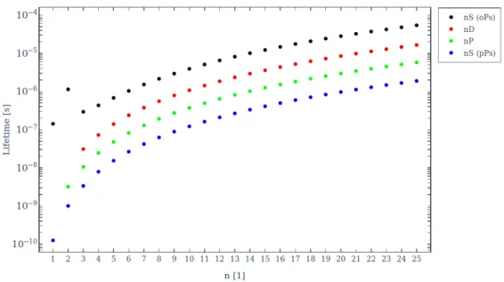
Figure 7 shows the lifetime (see equation 27) for S (L = 0), P (L = 1) and D (L = 2)

states. For S states with n > 1, the lifetime of pPs is dominated by annihilation due to it

decaying predominantly to two photons (see section 1.1.2), while oPs is mainly governed

by radiative decay. However, an important exception is oPs in the 2S state, which is

radiatively meta-stable. In fact, due to the small fine-structure splitting, the decay rate

Figure 7: Lifetime for positronium states with n < 26 including annihilation (for n < 3) and radiative decay. Numerical values for radiative lifetimes were taken from [39] and scaled by a factor 2 to account for the reduced mass.

to 2P is minuscule and the main contribution is the electric dipole transition directly to the 1S, by the simultaneous emission of two photons [40]. For P and D states the total spin does not play a significant role, since the radiative decay rates are many orders of magnitude larger than the respective annihilation decay rates.

1.2.3. The experimental history of positronium spectroscopy

From the very beginning of experimental efforts related to positronium, spectroscopic measurements were front and center. Just half a year after Deutsch published the first evidence for positronium formation in gases [7], he completed the first measurement of its hyperfine

structure [41]. The technique he developed served as a basis for virtually all subsequent hyperfine measurements in positronium.

Over the following decades the ground state hyperfine interval was measured with increasing precision [42–49], culminating in a 3.6 ppm measurement by Ritter et al. [50].

However, when theory calculations caught up in precision, it became clear that there was a discrepancy of almost 4 σ with those calculations. This prompted further experimental activity, including one of the measurements presented in this thesis (see chapter 4 for the recent history and current efforts).

The first experiment involving positronium in the excited state n = 2 [51] led to the measurement of the fine structure of positronium [52]. Subsequent measurements de- termined the different splittings [53–56] to varying accuracy, the most precise being the

10Note that there is historical ambiguity about the convention of naming the respective corrections in positronium fine or hyperfine structure. Over the years different authors used both those terms to describe the shift due to spin-spin coupling in positronium.

2

S

→ 2

P

(170 ppm) and the 2

S

→ 2

P

(225 ppm) transitions. The availabil- ity of slow positron beams and efficient laser excitation to the excited state allows for significant improvements on these measurements [57]. Most recently, a new (33 ppm) measurement of the 2

S

→ 2

P

interval showed a 4 . 5 σ discrepancy with the corre- sponding theoretical calculation [58]. This clearly shows the importance of additional, more precise measurements to be conducted. One such improvement is presented in chapter 4.

Finally, with the advent of high power, narrow-band lasers at the required wavelengths, optical spectroscopy of positronium was realized by Chu and Mills measuring the optical 1

S

→ 2

S

transition in 1982 [59]. This was continually improved upon, to be the benchmark QED test in positronium, reaching 12 ppb using pulsed lasers [60] and a final precision of 3.2 ppb [61–63] using CW lasers. After almost two decades of absence in positronium laser experiments, the last ten years saw a resurgence of experiments using lasers for a number of precise measurements in positronium (for an excellent overview see [57]). However, the 1993 value for the 1

S

→ 2

S

transition is still the most precise to date and significant improvements in our understanding of bound state QED (see preceding section) call for a new, more precise measurement of this transition. One such measurement is presented in chapter 3.

1.3. A window to the world beyond the Standard Model

The Standard Model of particle physics, which incorporates QED (and therefore also bound state QED), is an incredibly successful theoretical framework. It has led to many great insights into the makeup of our universe, culminating in the recent experimental discovery of the Higgs boson [64, 65]. Notwithstanding the success, it is clearly not the most fundamental description of nature, seeing as it neglects to describe one of the four known forces in nature – gravity. Furthermore, it does not explain phenomena such as dark matter, dark energy or the extreme baryon asymmetry in our universe.

A fundamental property of the Standard Model is that it is invariant under the com- bined transformations of C (charge), P (parity) and T (time). This is a consequence of the CP T -theorem [76, 77], which is valid in any quantum field theory respecting uni- tarity, Lorentz invariance and locality [78]. However, CP T invariance can be naturally broken in theories incorporating quantum gravity, e.g. string theory [79, 80].

Even if we do not know the “full” theory yet and scales at which it would become apparent are not accessible, effective field theories are a powerful tool to study the dynamics of a system at lower energy scales. In fact, in this context a quantum field theory might well be non-renormalizable but still have predictive power and operators of mass dimension d > 4 can be seen as an effective result of the unknown large energy scale dynamics [81].

One such effective field theory is the Standard Model Extension (SME), which as the

name suggests, is built as an extension to the Standard Model incorporating General

Relativity and all possible terms breaking Lorentz invariance [82]. Since a violation

of CP T implies Lorentz violation [83], the SME also includes terms breaking CP T

invariance. If the model is restricted to operators of mass dimension d ≤ 4, the theory

Energy [GeV]

10-27 10^-24 10^-21 10^-18 10^-15 10^-12 10^-9 10^-6 10^-3 1 10³

Energy [GHz]

10-12 10^-9 10^-6 10^-3 1 10³ 10⁶ 10⁹ 10¹² 10¹⁵

ν

H H-

1S-2S

ν H H-

2S-2P

ν H H-

1S-2S

Ps ν

2S-HFS

ν Ps

2S-2P₀

ν Ps

Figure 8: Sensitivity for CP T violation in hydrogen and positronium: The left edge of the bars represents the absolute accuracy of the respective measurements, while the right edge represents the absolute value. The length of the bar gives the relative precision. Solid bars are given for the most precise past measurements [55, 62, 66–68] in the exotic atom system – anti-hydrogen and positronium respectively – while non-filled bars represent expected accuracies [69–72] (see also chapter 3 and 4). Dotted bars show the most precise value in hydrogen [19, 73, 74]. ( adapted from: [75])

is renormalizable and referred to as the minimal Standard Model Extension.

The coefficients for Lorentz violation in the SME can not be found from first principles, but must be necessarily measured. Constraints for these coefficients have been extracted from a multitude of different experimental disciplines, including Astrophysics, particle colliders, optical experiments, and atomic spectroscopy [84]. Comparisons of atomic systems consisting of antimatter or a combination of matter and antimatter are excellent candidates to test CP T , due to the achievable precision in such experiments. Non- zero coefficients of Lorentz violating operators in the Standard Model extension lead to observable effects, such as shifts from bound state QED values and varying shifts depending on sidereal time [85].

In general, one is interested in measurements with the highest absolute precision and not the relative one, since all non-relativistic coefficients carry mass dimensions [85].

The most stringent limits are extracted from the hydrogen sector, but measurements in

positronium are competitive with anti-hydrogen (see figure 8). Furthermore, positron-

ium depends on a different combination of Lorentz violating coefficients than hydrogen,

allowing one to use the measurements to disentangle CP T -even and CP T -odd effects

[85]. In this sense positronium studies complement those in hydrogen and anti-hydrogen

respectively.

2. Pulsed slow positron beamline

2.1. Overview

The pulsed slow positron beamline at ETH Zurich (see figures 9 and 10) is designed to supply up to 10

positrons per second in nanosecond scale bunches at typically 1 Hz to 10 Hz repetition rate. The positron beam can be focused down to approximately 1 mm and guided onto a target to form positronium (details in section 3).

Figure 9: Schematic overview of the pulsed slow positron beamline at ETH Zurich. The drawing is not to scale and orientations might differ. For a detailed description of this part see section 2.1 and for an annotated picture of the physical setup, see figure 10. For further information about the pulsed beam handling up to the target implantation, refer to section 2.4 and figure 31.

Positrons are created in the β

decay of the radioactive isotope

Na and moderated using a solid rare gas moderator to approximately 40 eV. They are then guided through a velocity selector to remove unmoderated positrons from the beam, and further trans- ported to the buffer gas trap. Section 2.2 discusses this part of the beam in detail.

There they lose energy by inelastic collisions with N

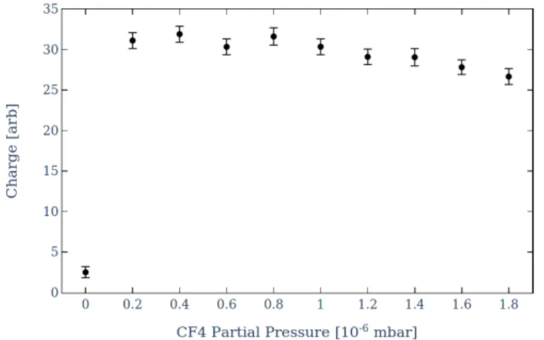
gas atoms to be trapped in an electric potential with magnetic radial confinement. In the last stage of the trap the positron plasma is compressed by a rotating electric field and cooled by collisions with CF

gas. A thorough description of the buffer gas trap can be found in section 2.3.

When the trap gate potential is opened, the cloud of positrons leaves the trap with

an energy on the order of 10 eV and is then magnetically guided to a drift tube, which

is pulsed to a potential of around 200 V to increase the beam energy. The positrons

are then transported through a beam extension of approximately 4 m, connecting the

buffer gas trap and the spectroscopy chamber in a dedicated laser room. Finally, a time-

varying potential on a second long cylindrical electrode compresses the time spread to a

few nanoseconds, before it is pulsed to high voltage. This accelerates the bunch to the

required implantation energy, which can be varied from approximately 1 keV to 6 keV,

depending on the experimental requirements. After leaving the electrode, the beam is extracted to a field-free region and focused spatially by an electrostatic einzel-lens. A more in-depth description of this stage can be found in section 2.4.

Figure 10: Picture of the pulsed slow positron beamline at ETH Zurich seen from the source side. The reimplantation electrode and source chamber are located in a separate room, which is connected by a transport section. The source chamber itself cannot be seen due to the radiation shielding that is required when the source is in place.

2.2. Positron source and moderation

Positrons are usually created using radioactive isotopes undergoing β

decay or by pair- production using accelerators. While accelerator [86, 87] and nuclear reactor [88, 89]

based systems offer high constant brightness sources of positrons, they are inherently limited to large facilities, difficult to operate and can be prohibitively expensive. There- fore, a large number of experimental efforts involving slow positron beams are employing a closed radioactive isotope source, which is easy to operate and mostly maintenance free. However, the drawback is that the activity is usually limited to around 2 GBq for radiation safety reasons and that the isotope decays according to its half-life (e.g. 951 days for

Na [90]) and needs to be replaced at regular intervals according to individual rate needs.

The source employed on the pulsed slow positron beamline at ETH Zurich is a com- mercial 463 MBq (January 2016)

Na capsule produced by iThemba LABS using a magnesium target irradiated by a 66 MeV proton beam and subsequent chemical ex- traction [91]. The titanium capsule (see figure 11) is closed and sealed after production.

Positrons can escape through a 5 µ m thick titanium foil covering the

Na salt deposition

on a tantalum reflector.

Figure 11: Picture (left) and drawing of

Na source capsule ( from: [91])

22 11

Na

950 . 97 d

22m10

Ne ( τ =3 . 2 ps)

2210

Ne β

1 . 82 MeV

0.06 %

β

0 . 54 MeV

89.84 %

1.27 MeV

22 11

Na

950 . 97 d

22m10

Ne ( τ =3 . 2 ps)

2210

Ne EC

0.001 %

EC

10.11 %

1.27 MeV

Figure 12: β

(left) and electron capture (right) decay channels of

Na including branching ratios and positron endpoint energies [92]

There are four relevant decay channels (see figure 12) for

Na. Positrons are emitted in approximately 90 % of all decays with endpoint energies of 546 keV (89 . 84 %) and 1821 keV (0 . 06 %), respectively [92]. The remaining decays proceed via electron capture and therefore do not contribute to the positron flux, which needs to be taken into account by appropriately scaling the activity, when calculating fluxes or efficiencies. Therefore, the scaled positron flux of the source is expected to be

Φ

( t ) = 0 . 9 · A

· e

≈ 416 × 10

· e

/

(31) where t is the age of the source in days. At the time of this writing (June 2020) the positron flux of the source is therefore taken to be approximately 126 × 10

/

. Note that this does not take losses on the reflector, window or bulk material of the source into account. This is usually included in the value of the moderator efficiency ε (see end of this section).

Since β -decay is a three body process, the positron energy is distributed over a wide

range. However, trapping requires a quite narrow energy spread on the order of a few eV (see section 2.3) and using positrons directly emitted from the source would be extremely inefficient. Therefore, a number of techniques to moderate beams of positrons have been developed, which reduce the mean positron energy drastically (see figure 14). However, the drawback with all these methods is that they are quite inefficient due to the high probability of annihilation of positrons on matter. The ideal moderator for a given application depends on the requirements on the achievable efficiency and energy spread [93].

The most common choices in transmission geometry are metal foil/mesh (most com- monly Ni or W) or solid rare gas moderators (most commonly Kr, Ar or Ne). With appropriate preparation and annealing procedures, tungsten foils or meshes can reach efficiencies of ε ≈ 0 . 1 % and an energy spread on the order of a few hundred meV [94, 95].

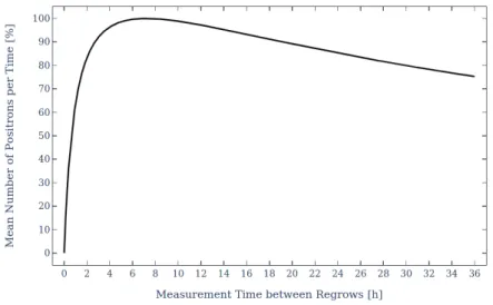
Solid neon moderators [96] are able to provide efficiencies which are an order of magni- tude higher at the cost of a slightly larger energy spread of approximately 2 eV and the additional requirement for a cryogenic system, capable of achieving temperatures below approximately 8 K. The slightly larger energy spread results in a loss of achievable trap- ping efficiencies (see section 2.3) of around a factor 2 [97], but this is more than offset by the increase in moderator efficiency. Contrary to metal moderators, solid rare gas moderators tend to degrade over time and need to be regularly regrown (see below in this section).

Positrons implanted in metals rapidly thermalize to approximately 40 meV (room tem- perature) by inelastic collisions on a picosecond timescale and can be reemitted from the surface after diffusion, if the metal has a negative positron workfunction [93]. In solid rare gases however, positrons will lose energy efficiently only down to a certain threshold energy below which the only loss mechanism proceeds via very inefficient phonon emis- sion [96]. The diffusion length and the moderation efficiency is therefore higher in these materials. Due to the fact that most of these positrons are not completely thermalized, the energy spread is correspondingly higher.

The pulsed slow positron beam at ETH Zurich employs a cryogenic solid rare gas moderator using neon or alternatively argon

. An overview of the moderator assembly can be found in figure 13. The source is mounted on the second stage of an ARS DE-204 closed cycle cryocooler capable of reaching 4 K with a cooling power of 0 . 2 W at 4 . 2 K via a sapphire disc. This allows for good thermal contact, while providing electrical isolation for applying a bias voltage to the source. The source is placed in such a way that the window is flush with a conical aperture where a film of solid rare gas is frozen onto. This geometry allows for strongly increased moderation efficiencies [98].

An overview of the main elements of the slow pulsed positron beam can be found in figure 10. A CF160 turbopump (Pfeiffer HiPace 700M - approximately 700 l / s pumping speed) is mounted directly on top of the source chamber. A second chamber, connected by a CF16 pumping restriction (ID 16 mm), is pumped separately by a CF100 turbo- pump (Pfeiffer HiPace 300M - approximately 250 l / s pumping speed). This chamber is

11Argon can be used to extend the service lifetime of the coldhead, since it allows for temperatures significantly higher than neon, at the cost of around a factor 4 to 5 of moderation efficiency.

Figure 13: Picture of coldhead assembly with mounted heat shield, source holder and mount (left) and CAD drawing of cross-section of source holder in mount with with moderator cone (right). Note that the wire heater shown here was exchanged for a kapton foil heater in the current configuration.

connected to the trapping region by another CF16 restriction and a gate valve. This setup allows for continuous operation of all pumps, even while evaporating and growing the moderator. Furthermore, the gate valve to the trapping chamber can be left open during all phases, with only minor impact on operating pressures. The final pressure

reached during operation is below 5 × 10

mbar.

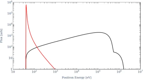
Figure 14: Calculated energy distribution of unmoderated (black) and solid neon mod- erated (red, assuming a Landau distribution) positrons in

Na β

decay for 40 V source voltage and 0 . 5 % moderation efficiency

To monitor the parameters and performance several detectors are placed along the

12The employed pressure sensor (Pfeiffer PKR 261) shows a minimum pressure of 5×10⁻⁹mbar, so the achievable end pressure is likely significantly lower.

beamline (see figure 9). Both before the trap inlet and after the trap outlet a large solid angle plastic scintillator, coupled to a photo-multiplier tube (PMT), is placed close to the respective gate valve, which can be closed to serve as an annihilation plate. Additionally, two fully shielded custom design multi channel plate (MCP) detectors can be inserted into the beam path by means of linear actuators. Both MCP mounts incorporate a grid electrode that can be used to bias off moderated positrons of arbitrary energy.

The detector on the trap outlet side can be used both in CW and pulsed mode and is also equipped with a phosphor screen to allow for visual inspection and beam size measurements.

To determine the total rate of positrons, or equivalently the moderation efficiency, the scintillator at the trap inlet was calibrated for rate and solid angle using a radioactive source. To measure the losses due to magnetic mirroring on the trap solenoid, another scintillator was placed at the trap outlet and likewise calibrated. A lead tungstate (PbWO

) scintillator

was additionally placed there to determine the trapping efficiency in pulsed mode (see section 2.3).

For the calibration of the scintillators a closed

Na source with an activity of A

( t = 4505 d) = A

· e

≈ 413 kBq · e

= 15 . 46 kBq (32) was used. The fractional coverage is given by

ω = 4 π

Ω (33)

where Ω is the subtended solid angle of the scintillator. While the detection efficiency often strongly depends on the incident energy of the particle, for the used group of plastic scintillators and range of energies the response is quite flat [99–101] and one can assume the same detection efficiency ε

for all photons. Therefore, the discussion of the calibration factor can be limited to the probability to pick up at least one photon from either a beam positron annihilation or one

Na decay of the calibration source. The measured rate from beam positrons is given by

R

= ε

N

· [1 − (1 − 2 · ω )] = 2 ωε

N

(34) where N

is the rate of positrons on the annihilation point. On the other hand, one needs to correct for the fact that in addition to the 511 keV photons from positron annihilation, the calibration source additionally emits a 1275 keV neon de-excitation gamma. Additionally, approximately 10 % of the

Na decays of the calibration source proceed via electron capture without the emission of 511 keV gammas (see figure 12).

The rate for the calibration source is therefore given by

R

= ε

A

{ 1 − [0.1(1 − ω) + 0.9(1 − ω)(1 − 2ω)] } = 2ωε

A

(1.4 − 0.9ω) (35)

13Multiple lead tungstate scintillators were graciously supplied by Dr. Nessi-Tedaldi of the ETH CMS group.

and for the special case of the calibration source directly placed on top of the scintillator ( ω ≈ 0 . 5):

R

= R

( d = 0) = ε

A

· 0 . 95 (36) with d being the distance between source and scintillator.

Therefore three count rate measurements are needed to calculate the calibration factor, namely one with the calibration source placed directly on top of the scintillator centred on the active area ( R

), one with the source placed at the distance of the annihilation point ( R

), and one measurement without source and moderator grown ( R

). The fractional coverage can be calculated from the ratio

R

R

= 2.8ω − 1.8ω

0 . 95 ⇒ ω = 2.8 −

7.84 − 6.84

3 . 6 (37)

and the detection efficiency

ε

= R

0 . 95 A

(38)

then gives the calibration factor

CF = N

R

= 1

2 ωε

= 0 . 95 A

2 ωR

(39)

which has to be multiplied with the count rate to arrive at the total positron rate annihilating close to the scintillator position. Uncertainties in the exact position of the annihilation point result in errors on the order of 15 % for the calibration factor. This is purely a scale error and can be neglected for comparing various growth parameters, but has to be included for absolute values, e.g. the moderation efficiency.

The calibration factors for the scintillators were found to be

CF

= 67 ± 10 (40)

and

CF

= 23.0 ± 3.4 (41)

for the scintillators placed before the trap inlet and after the trap outlet respectively.

A typical procedure to prepare the solid neon moderator is shown in figure 15 and consists of four distinct phases. In the first phase (evaporation) the second stage is heated up via a 50 Ω kapton foil heater, mounted to the second stage of the closed cycle cryostat, to a peak temperature of approximately 40 K.

This leads to the evaporation and pumping out of the old neon moderator. Additionally, the neon line is flushed to ensure that there are no impurities which would impact the quality of the fresh moderator.

The flow rate is set such that the chamber pressure does not exceed 10

mbar to avoid

14This is a good approximation due to the small size of the source relative to the large surface area of the scintillator.

15Note that at this temperature not all gas species completely evaporate. To avoid degrading moderator performance due to buildup of other gas species, the second stage is heated to approximately 80 K at regular intervals, i.e. after 20 - 30 regrowth cycles.