Universit¨ at Regensburg Mathematik
Stable variational approximations of boundary value problems for
Willmore flow with Gaussian curvature
John W. Barrett, Harald Garcke and Robert N¨ urnberg
Preprint Nr. 01/2016
Stable variational approximations of boundary value problems for Willmore flow with Gaussian curvature
John W. Barrett
†Harald Garcke
‡Robert N¨ urnberg
†Abstract
We study numerical approximations for geometric evolution equations arising as gradient flows for energy functionals that are quadratic in the principal curvatures of a two-dimensional surface. Beside the well-known Willmore and Helfrich flows we will also consider flows involving the Gaussian curvature of the surface. Boundary conditions for these flows are highly nonlinear, and we use a variational approach to derive weak formulations, which naturally can be discretized with the help of a mixed finite element method. Our approach uses a parametric finite element method, which can be shown to lead to good mesh properties. We prove stability estimates for a semidiscrete (discrete in space, continuous in time) version of the method and show existence and uniqueness results in the fully discrete case. Finally, several numerical results are presented involving convergence tests as well as the first computations with Gaussian curvature and/or free or semi-free boundary conditions.
Key words. Willmore flow, parametric finite elements, tangential movement, spon- taneous curvature, clamped boundary conditions, Navier boundary conditions, Gaussian curvature energy, line energy.
AMS subject classifications. 65M60, 65M12, 35K55, 53C44
1 Introduction
Energies involving the principal curvatures of a two-dimensional surface in the three dimensional Euclidean space play an important role in geometry, physics, biology and imaging. The Willmore energy given as the integrated square of the mean curvatures is of great interest in geometry, cf. Willmore (1993). However, also more general functionals involving the principal curvatures appear in the theory of elastic plates and shells, and go back to work of Poisson (1812), Germain (1821) and Kirchhoff (1850). In the theory of biological membranes the work of Helfrich (1973) used generalized curvature functionals, which lead to a huge interest for curvature functionals in the field of biophysics. Boundary
†Department of Mathematics, Imperial College London, London, SW7 2AZ, UK
‡Fakult¨at f¨ur Mathematik, Universit¨at Regensburg, 93040 Regensburg, Germany
value problems involving curvature functionals also play an important role in imaging, for example in problems involving surface restoration and image inpainting, cf. Clarenz et al. (2004); Bobenko and Schr¨oder (2005). Analytical and numerical work on static and evolutionary questions in the context of curvature functionals so far have been mainly focused on the case of closed surfaces, and we refer to Simon (1993); Kuwert and Sch¨atzle (2001); Rivi`ere (2008); Marques and Neves (2014) for analytical results, and to Mayer and Simonett (2002); Rusu (2006); Dziuk (2008); Barrett et al. (2008) for numerical results.
Much less is known for boundary value problems involving functionals that include cur- vature quantities. Analytical results often need small data assumptions, use symmetries or consider the graph case. We refer to Nitsche (1993); Bergner et al. (2009); Dall’Acqua et al. (2008); Deckelnick and Grunau (2009); Sch¨atzle (2010); Deckelnick et al. (2015) for the static case and to Abels et al. (2016) for an evolution problem for the Willmore energy with boundary conditions. Numerical approaches to problems involving the Will- more energy and boundary conditions are discussed in Peres Hari et al. (2001); Clarenz et al. (2004); Bobenko and Schr¨oder (2005); Deckelnick et al. (2015). In this context we refer to Wang and Du (2008), see also Du (2011), who used a phase field approach to study open membranes numerically.
Experimental observations for open membranes are reported in Saitoh et al. (1998).
Capovilla and Guven (2004); Tu and Ou-Yang (2003) and Biria et al. (2013) used vari- ational calculus to derive equilibrium equations for a bilayer membrane having an edge, and also provided physical interpretations of the equations obtained.
To the knowledge of the authors, no results are available in the literature so far for numerical approaches of evolution problems that involve also the Gaussian curvature and/or free or semi-free boundary conditions. It is the goal of this paper to derive and analyze a finite element approximation of L2–gradient flows for curvature functionals of Willmore and Helfrich type that allow also for Gaussian curvature and (semi-)free boundary conditions. We are interested in discretizations which allow to treat the highly nonlinear boundary conditions in a variational way, which will then make it possible to derive stability estimates. In order to do so, it is necessary to generalize work of Dziuk (2008) and Barrett et al. (2016) on computational Willmore flow for closed surfaces to the case of open surfaces. Due to the highly nonlinear boundary conditions, this is a nontrivial task.
In order to formulate the governing problems in more detail, we parameterize the surfaces over a fixed oriented, compact, smooth reference manifold Υ ⊂R3 with boundary
∂Υ. We now consider a hypersurface Γ with boundary ∂Γ parameterized by~x : Υ→R3 with normal ~ν given by the orientation. Denoting by ∇s = (∂s1, ∂s2, ∂s3) the surface gradient on Γ we define∇sχ~ = ∂sjχi
3 i,j=1.
We then define the second fundamental tensor for Γ as ∇s~ν, and we recall that
−∇s~ν(~z), for any ~z ∈ Γ, is a symmetric linear map that has a zero eigenvalue with eigenvector ~ν. The remaining two eigenvalues, κ1,κ2, are the principal curvatures of Γ at ~z; see e.g. (Deckelnick et al., 2005, p. 152). Hence −∇s~ν(~z) induces a linear map S : T~zΓ → T~zΓ on the tangent space T~zΓ for any ~z ∈ Γ. The map −S is called the
Weingarten map or shape operator. The mean curvature κ and the Gaussian curvature K can now be stated as
κ= trS =κ1 +κ2 and K= det (S) =κ1κ2, (1.1) where we note that unit spheres with outer unit normal have mean curvatureκ =−2. It then follows that |∇s~ν|2 =κ2
1+κ2
2 =κ2−2K. The mean curvature vector is given as
∆sid =~ κ~ν =:~κ on Γ, (1.2)
where ∆s =∇s.∇s is the Laplace–Beltrami operator on Γ.
The Willmore energy is now given as E0(Γ) := 12
Z
Γ
κ2 dH2 = 12 Z
Γ|κ~|2 dH2, (1.3) see e.g. Willmore (1993) for details. Here and throughout Hd, d = 1,2, denotes the d- dimensional Hausdorff measure. Realistic models for biological cell membranes lead to energies more general than (1.3). In the original derivation of Helfrich (1973) a possible asymmetry in the membrane, originating e.g. from a different chemical environment, was taken into account. This lead Helfrich to the energy
Eκ(Γ) = 12 Z
Γ
(κ−κ)2 dH2 = 12 Z
Γ|~κ−κ~ν|2 dH2, (1.4) where κ ∈ R is the given so-called spontaneous curvature. Similarly to Barrett et al.
(2016), we will also consider the energy
Eκ,β(Γ) :=Eκ(Γ) + β2 (M(Γ)−M0)2 (1.5a) with
M(Γ) = Z
Γ
κdH2 = Z
Γ
~
κ. ~ν dH2 (1.5b)
and given constants β ∈ R≥0, M0 ∈ R. Models employing the energy (1.5a) are often called area-difference elasticity (ADE) models, see Seifert (1997). We note that for present models, choosing β > 0 does not have a physically meaningful interpretation for surfaces with boundary.
For open surfaces also contributions taking Gaussian curvature and line energy into account are relevant. We hence consider
E(Γ) :=Eκ,β(Γ) +αG
Z
ΓKdH2+γH1(∂Γ), (1.6) for given αG ∈R and γ ∈R≥0.
Similarly to (1.2), fundamental to many approaches, which numerically approximate evolving curves in a parametric way, is the identity
id~ss=~κ∂Γ on ∂Γ, (1.7)
whereκ~∂Γ is the curvature vector on ∂Γ. Here we choose the arclength sof the curve ∂Γ such that (id~s, ~µ, ~ν), where
~µ=~ν×id~s on ∂Γ (1.8)
denotes the conormal to Γ on ∂Γ, form a positively oriented orthonormal basis of R3. Note that ~µis a vector that is perpendicular to the unit tangent id~s on∂Γ and lies in the tangent space of Γ. Now (1.7) can be rewritten as
id~ss=κ~∂Γ =κµ~µ+κν~ν on ∂Γ, (1.9) where κµ is the geodesic curvature and κν is the normal curvature. It then follows from the Gauß–Bonnet theorem,
Z
ΓKdH2 = 2π m(Γ) + Z
∂Γ
κµdH1, (1.10)
wherem(Γ)∈Zdenotes the Euler characteristic of Γ, that the energy (1.6), is equivalent to
E(Γ) := Eκ,β(Γ) +αG
Z
∂Γ
~
κ∂Γ. ~µdH1+ 2π m(Γ)
+γH1(∂Γ). (1.11) It turns out that the first variation of the energy is given by, compare (A.49) in the appendix, Nitsche (1993) and Barrett et al. (2016),
∆sκ−(12(κ−κ)2+β(M(Γ)−M0)κ)κ+ (κ−κ+β(M(Γ)−M0))|∇s~ν|2, and the gradient flow dynamics hence moves a point on the surface Γ with a normal velocity which is the negative of the above expression.
The gradient flow is hence given as a family (Γ(t))t∈[0,T] of evolving surfaces with boundary ∂Γ(t) that are parameterized by ~x(·, t) : Υ→R3 for which
V =−∆sκ+ (12(κ−κ)2+β Aκ)κ−(κ−κ+β A)|∇s~ν|2 (1.12) holds, where
A=M(Γ(t))−M0. (1.13)
Here V~(~z, t) :=~xt(~q, t) ∀ ~z=~x(~q, t)∈Γ(t) (1.14) defines the velocity of Γ(t), and V := ~V. ~ν is the normal velocity of the evolving hyper- surface Γ(t). The flow (1.12) is of fourth order (taking into account that κ involves two derivatives of the parameterization).
In this paper, we consider four different types of boundary conditions on ∂Γ(t). The boundary ∂Γ(t) can either move freely, or move along the boundary of a fixed domain Ω, or it will be fixed, ∂Γ(t) =∂Γ(0). For the latter case two types of boundary conditions arise: clamped and Navier. As noted earlier, the flow (1.12) is a highly nonlinear fourth order parabolic partial differential equation for the parameterization ~x. Hence, if the boundary of Γ(t) is fixed, two boundary conditions are needed in order to yield a well- posed problem. If the boundary Γ(t) can move, however, then an additional boundary
condition is needed to close the system. Similarly to Barrett et al. (2012, Remark 2.1), we may write Γ(t) locally near the boundary as a graph over a time-dependent domainD(t).
The fact that ∂D(t) can move shows the need for three boundary conditions to obtain a well-posed problem. In the free boundary case, the three necessary boundary conditions are given by
(∇sκ). ~µ+γκν −αGτs = 0 on ∂Γ(t), (1.15a)
−12 (κ−κ)2−β Aκ+γκµ−αGK= 0 on ∂Γ(t), (1.15b) κ−κ+β A+αGκν = 0 on ∂Γ(t), (1.15c) where τ denotes the torsion of the curve ∂Γ(t), see the appendix for a derivation. We note that in the case β = γ =αG = 0 the condition (1.15b) collapses to (1.15c), and so we conjecture that for this choice of parameters the evolution problem is not well posed.
For the partially free case, when ∂Γ(t)⊂∂Ω for all t ∈[0, T], where ∂Ω is the boundary of a fixed open domain Ω⊂R3, we let ∂Ω be given by a function F ∈C1(R3) such that
∂Ω ={~z∈R3 :F(~z) = 0} and |∇F(~z)|= 1 ∀~z∈∂Ω,
and we denote the normal to Ω on∂Ω by~n∂Ω =∇F. The necessary boundary conditions are then
∂Γ(t)⊂∂Ω (1.16a)
[(∇sκ). ~µ+γκν −αGτs] (~µ . ~n∂Ω)−[−12(κ−κ)2−β Aκ+γκµ−αGK] (~ν . ~n∂Ω) = 0 on ∂Γ(t), (1.16b)
κ−κ+β A+αGκν = 0 on ∂Γ(t), (1.16c)
see the appendix for a derivation. Clamped boundary conditions are given by
∂Γ(t) =∂Γ(0) and ~µ(t) =~ζ(t) on ∂Γ(0), (1.17) where ~ζ∈C([0, T], C(∂Γ(0),Sd−1)). Similarly, Navier boundary conditions are given by
∂Γ(t) =∂Γ(0) and κ =κ−β A−αGκν on∂Γ(0), (1.18) see the appendix for a derivation. Of course, for the two fixed boundary conditions, when
∂Γ(t) = ∂Γ(0) for t ≥ 0, the line energy contributions in (1.11) play no role. Similarly, for clamped boundary conditions, (1.17), the last integral in (1.11) is fully determined by the data, and so Gaussian curvature plays no role in this case.
In some cases, in particular in applications for biomembranes, cf. Tu (2013), the surface area of Γ needs to stay constant during the evolution. In this case one can consider
Eλ(Γ) =E(Γ) +λH2(Γ) (1.19)
has to be considered. Here, λ is a Lagrange multiplier for the area constraint, which can be interpreted as a surface tension. In this case (1.12) is replaced by
V =−∆sκ+ (12(κ−κ)2+β Aκ)κ−(κ−κ+β A)|∇s~ν|2+λκ, (1.20)
and (1.15b) is replaced by
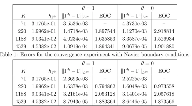
−12(κ−κ)2−β Aκ+γκµ−αGK=λ on ∂Γ(t). (1.21) In Section 2 we will derive a weak formulation for the continuous problem. This will be the basis for the semidiscrete finite element approximation introduced in Section 3 for which we can show a stability result. In Section 4 we formulate a fully discrete finite element approximation for which we can show that a unique solution exists. After a discussion on how to solve the fully discrete linear algebra problem in Section 5, we present in Section 6 several numerical results, many of them for situations for which no computations were available beforehand.
2 Weak formulations/Formal calculus of PDE con- strained optimization
On recalling (1.14), we define the following time derivative that follows the parameteri- zation~x(·, t) of Γ(t). Let
∂t◦φ =φt+V~.∇φ ∀φ ∈H1(GT), (2.1) where we have defined the space-time surface
GT := [
t∈[0,T]
Γ(t)× {t}. (2.2)
Here we stress that this definition is well-defined, even though φt and ∇φ do not make sense separately for a function φ∈H1(GT). For later use we note that
d
dthψ, φiΓ(t) =h∂t◦ψ, φiΓ(t)+hψ, ∂t◦φiΓ(t)+D
ψ φ,∇s. ~VE
Γ(t) ∀ ψ, φ∈H1(GT), (2.3) see Lemma 5.2 in Dziuk and Elliott (2013). Here h·,·iΓ(t) denotes the L2–inner product on Γ(t). It immediately follows from (2.3) that
d
dtH2(Γ(t)) =D
∇s. ~V,1E
Γ(t) =D
∇sid,~ ∇sV~E
Γ(t). (2.4)
In this section we would like to derive a weak formulation for the L2–gradient flow of E(Γ(t)). To this end, we need to consider variations of the energy with respect to Γ(t) =~x(Υ, t). For any given χ~ ∈[H1(Γ(t))]3 and for any ε ∈(0, ε0) for some ε0 ∈R>0, let
Γε(t) :={Ψ(~z, ε) :~ ~z∈Γ(t)}, where Ψ(~z,~ 0) =~z and ∂ ~∂εΨ(~z,0) =χ(~z)~ ∀ ~z∈Γ(t). (2.5)
We note that in the case of a fixed boundary, we choose variations χ~ ∈ [H01(Γ(t))]3, and so ∂Γε(t) = ∂Γ(t) = ∂Γ(0). The first variation of H2(Γ(t)) with respect to Γ(t) in the direction χ~ ∈[H1(Γ(t))]3 is given by
δ
δΓH2(Γ(t))
(~χ) = d
dεH2(Γε(t))|ε=0
= lim
ε→0 1 ε
H2(Γε(t))− H2(Γ(t))
=D
∇sid,~ ∇sχ~E
Γ(t), (2.6) see e.g. the proof of Lemma 1 in Dziuk (2008). For later use we note that generalized variants of (2.6) also hold. Namely, we have that
δ
δΓhw,1iΓ(t)
(~χ) = d
dεhwε,1iΓε(t) |ε=0=D
w∇sid,~ ∇sχ~E
Γ(t) ∀w∈L∞(Γ(t)), (2.7) where wε ∈L∞(Γε(t)), for any w∈L∞(Γ(t)), is defined by
wε(Ψ(~z, ε)) =~ w(~z) ∀~z ∈Γ(t), (2.8) and similarly for w~ ∈[L∞(Γ(t))]3. This definition ofwε yields that ∂ε0w= 0, where
∂ε0w(~z) = d
dεwε(Ψ(~z, ε))~ |ε=0 ∀ ~z∈Γ(t). (2.9) Of course, (2.7) is the first variation analogue of (2.3) with w=ψ φ and ∂ε0ψ =∂ε0φ = 0.
Similarly, it holds that δ
δΓhw, ~ν~ iΓ(t)
(~χ) = d
dε hw~ε, ~νεiΓε(t) |ε=0=D
(w . ~ν)~ ∇sid,~ ∇sχ~E
Γ(t)+
~ w, ∂ε0~ν
Γ(t)
∀ w~ ∈[L∞(Γ(t))]3, (2.10) where ∂ε0w~ = ~0 and ~νε(t) denotes the unit normal on Γε(t). In this regard, we note the following result concerning the variation of ~ν, with respect to Γ(t), in the direction
~
χ∈[H1(Γ(t))]3:
∂ε0~ν =−[∇sχ]~ T~ν on Γ(t) ⇒ ∂◦t~ν =−[∇sV~]T~ν on Γ(t), (2.11) see Schmidt and Schulz (2010, Lemma 9). Finally, we note that for ~η ∈ [H1(Γ(t))]3 it holds that
δ δΓ
D∇sid,~ ∇s~ηE
Γ(t)
(~χ) = d dε
D∇sid,~ ∇s~ηε
E
Γε(t) |ε=0=h∇s. ~η,∇s. ~χiΓ(t)
+ X3
l, m=1
hh(~ν)l(~ν)m∇s(~η)m,∇s(~χ)liΓ(t)− h(∇s)m(~η)l,(∇s)l(~χ)miΓ(t)
i
=h∇s~η,∇s~χiΓ(t)+h∇s. ~η,∇s. ~χiΓ(t)−D
(∇s~η)T, D(~χ) (∇sid)~ TE
Γ(t), (2.12)
where ∂ε0~η=~0, see Lemma 2 and the proof of Lemma 3 in Dziuk (2008). Here
D(~χ) :=∇s~χ+ (∇s~χ)T , (2.13) and we note that our notation is such that ∇s~χ = (∇Γχ)~ T, with ∇Γχ~ = (∂siχj)3i,j=1 defined as in Dziuk (2008). It follows from (2.12) that
d dt
D
∇sid,~ ∇s~ηE
Γ(t) =D
∇s~η,∇sV~E
Γ(t)+D
∇s. ~η,∇s. ~VE
Γ(t)−D
(∇s~η)T, D(V~) (∇sid)~ TE
Γ(t)
∀ ~η∈ {~ξ∈H1(GT) :∂◦t ~ξ=~0}. (2.14) For closed surfaces, in the seminal work Dziuk (2008), the author introduced a stable semidiscrete finite element approximation of Willmore flow, which is based on the discrete analogue of the identity 12 dtd hκ~, ~κiΓ(t) =−D
f~Γ, ~VE
Γ(t), where Df~Γ, ~χE
Γ(t) =h∇sκ~,∇sχ~iΓ(t)+h∇s. ~κ,∇s. ~χiΓ(t)−D
(∇sκ~)T, D(~χ) (∇sid)~ TE
Γ(t)
+12D
|κ~|2∇sid,~ ∇sχ~E
Γ(t) ∀χ~ ∈[H1(Γ(t))]3. (2.15) In the recent paper Barrett et al. (2015a) the present authors were able to extend (2.15), and the corresponding semidiscrete approximation, to the case of nonzero β and κ in (1.5a). The approximation is based on a suitable weak formulation, which can be ob- tained by considering the first variation of (1.5a) subject to the side constraint, the weak formulation of (1.2),
hκ~, ~ηiΓ(t)+D
∇sid,~ ∇s~ηE
Γ(t) = 0 ∀ ~η∈[H1(Γ(t))]3. (2.16) To this end, one defines the Lagrangian
L(Γ(t), ~e κ, ~y) = 12
|~κ−κ~ν|2,1
Γ(t)+ β2
h~κ, ~νiΓ(t)−M0
2
− h~κ, ~yiΓ(t)−D
∇sid,~ ∇s~yE
Γ(t)
(2.17) with ~y ∈ [H1(Γ(t))]3 being a Lagrange multiplier for (2.16). Then, on using ideas from the formal calculus of PDE constrained optimization, see e.g. Tr¨oltzsch (2010), one can compute the direction of steepest descent f~Γ of Eκ,β(Γ(t)), under the constraint (2.16).
In particular, we formally require that δ
δΓLe
(~χ) = lim
ε→0 1 ε
hL(Γe ε(t), ~κ, ~y)−L(Γ(t), ~e κ, ~y)i
=−D f~Γ, ~χE
Γ(t), (2.18a) δ
δ~κ Le
(~ξ) = lim
ε→0 1 ε
hL(Γ(t), ~e κ+ε ~ξ, ~y)−L(Γ(t), ~e κ, ~y)i
= 0, (2.18b)
δ δ~yLe
(~η) = lim
ε→0 1 ε
hL(Γ(t), ~e κ, ~y+ε ~η)−L(Γ(t), ~e κ, ~y)i
= 0. (2.18c)
On recalling (2.7)–(2.12), this yields that 12 dtdEκ,β(Γ(t)) =−D f~Γ, ~VE
Γ(t), where Df~Γ, ~χE
Γ(t) =h∇s~y,∇sχ~iΓ(t)+h∇s. ~y,∇s. ~χiΓ(t)−D
(∇s~y)T, D(~χ) (∇sid)~ TE
Γ(t)
−12
D
[|κ~ −κ~ν|2−2 (~y . ~κ)]∇sid,~ ∇sχ~E
Γ(t)+ (β A−κ)
~
κ,[∇sχ]~ T ~ν
Γ(t)
−β AD
(~κ. ~ν)∇sid,~ ∇sχ~E
Γ(t) = 0 ∀χ~ ∈[H1(Γ(t))]3, (2.19a) D
~
κ+ (β A−κ)~ν−~y, ~ξE
Γ(t) = 0 ∀ ~ξ ∈[H1(Γ(t))]3, (2.19b) h~κ, ~ηiΓ(t)+D
∇sid,~ ∇s~ηE
Γ(t) = 0 ∀ ~η ∈[H1(Γ(t))]3, (2.19c) where
A(t) =h~κ, ~νiΓ(t)−M0. (2.19d) Clearly, (2.19b) implies thatκ~+ (β A−κ)~ν =~y. In the caseκ =β= 0, this collapses to
~y=~κ, and so (2.19a) collapses to (2.15). In the context of the numerical approximation of the L2–gradient flow ofEκ,β(Γ(t)), (2.19a–d) gives rise to the following weak formulation, where we recall (1.14). Given Γ(0), for all t ∈ (0, T] find Γ(t) = ~x(Υ, t), with V~(t) ∈ [H1(Γ(t))]3, and~y(t)∈[H1(Γ(t))]3 such that (2.19a) holds with κ~ =~y−(β A−κ)~ν and A(t) =h~κ, ~νiΓ(t)−M0, and such that
DV −~ f~Γ, ~χE
Γ(t)= 0 ∀ χ~ ∈[H1(Γ(t))]3, (2.20a)
h~y, ~ηiΓ(t)+D
∇sid,~ ∇s~ηE
Γ(t) = (β A−κ)h~ν, ~ηiΓ(t) ∀ ~η∈[H1(Γ(t))]3. (2.20b) Under discretization, (2.20a,b) does not have good mesh properties. That is because the discretizations will exhibit mesh movements that are almost exclusively in the normal direction, which in general leads to bad meshes. To see this, we note that (2.20a,b) is the weak formulation of
V~ =
−∆sκ+ (12(κ−κ)2+β Aκ)κ− |∇s~ν|2(κ−κ+β A)
~ν , (2.21) which agrees with Barrett et al. (2008, (1.12)). A derivation of (2.21) is given in the ap- pendix. In order to overcome the undesirable mesh effects for a discretization of (2.20a,b), the authors in Barrett et al. (2016) replaced the side constraint (2.16) with the more gen- eral side constraint
DQθκ~, ~ηE
Γ(t)+D
∇sid,~ ∇s~ηE
Γ(t) = 0 ∀ ~η∈[H1(Γ(t))]3, (2.22) where θ∈[0,1] is a fixed parameter, and where Qθ is defined by
Qθ =θId + (1−θ)~ν⊗~ν on Γ(t). (2.23) On recalling (1.2), we note that on the continuous level (2.22) trivially holds independently of the choice of θ ∈ [0,1]. However, on the discrete level (2.22), for θ < 1, leads to an
induced tangential motion and good meshes, in general. See e.g. (3.39) in Section 3 below for more details.
From now on we consider open surfaces. Then, similarly to (2.22), we consider the side constraint
DQθ~κ, ~ηE
Γ(t)+D
∇sid,~ ∇s~ηE
Γ(t) =hm, ~η~ i∂Γ(t) ∀ ~η∈[H1(Γ(t))]3, (2.24) which again holds trivially on the continuous level for m being the conormal~ ~µ. Here h·,·i∂Γ(t) denotes the L2–inner product on ∂Γ(t). We stress that in the clamped case,
∂Γ(t) =∂Γ(0) and m =~ ~µ=~ζ in (2.24) are fixed given data, recall (1.17). For the other three types of boundary conditions, (2.24) weakly defines the conormal ~µ(t) to Γ(t) on
∂Γ(t). In the discrete setting, the discrete analogue of (2.24) will weakly define a discrete conormalm~h(t), which will in general be different from the true conormal~µh(t) to Γh(t) on
∂Γh(t), defined via the discrete analogue of (1.8), where Γh(t) is a discrete approximation of Γ(t).
Similarly to (2.16), and for later use, we introduce the weak formulation of (1.7): Find
~
κ∂Γ ∈[H1(∂Γ(t))]3 such that h~κ∂Γ, ~ηi∂Γ(t)+D
id~s, ~ηs
E
∂Γ(t) = 0 ∀~η ∈[H1(∂Γ(t))]3. (2.25) Similarly to (2.7) it holds that
δ
δΓhw,1i∂Γ(t)
(~χ) = d
dεhwε,1i∂Γε(t) |ε=0=D
w ~ids, ~χs
E
∂Γ(t)
∀ w∈L∞(∂Γ(t)), ~χ∈[H∂Γ1 (Γ(t))]3, (2.26) where ∂ε0w~ =~0, and where
H∂Γ1 (Γ(t)) :={η∈H1(Γ(t)) :η|∂Γ(t)∈H1(∂Γ(t))}. (2.27) Moreover, similarly to (2.12), we note that for~η ∈[H∂Γ1 (Γ(t))]3 it holds that
δ δΓ
Did~s, ~ηs
E
∂Γ(t)
(~χ) =
P∂Γ~ηs, ~χs
∂Γ(t) , (2.28)
where ∂ε0~η=~0, and where
P∂Γ = Id−id~s⊗id~s on ∂Γ(t). (2.29) For notational convenience, we also define
[H∇1F(Γ(t))]3 ={~η∈[H∂Γ1 (Γ(t))]3 :~η .∇F = 0 on ∂Γ(t)} (2.30) and
X(Γ(t)) =
[H∂Γ1 (Γ(t))]3 free boundary conditions, [H∇1F(Γ(t))]3 semi-free boundary conditions, [H01(Γ(t))]3 fixed boundary conditions.
(2.31)
We first consider the three types of boundary conditions that do not involve fixing the conormal on ∂Γ(t), i.e. free, semi-free and Navier. We recall the energy (1.11) and the fact that m(Γ(t)) is a topological invariant, which does not change its value under continuous deformations of the surface Γ(t). We hence define the Lagrangian omitting the term m(Γ(t)) as follows. Let
L(Γ(t), ~κ, ~m, ~κ∂Γ, ~y, ~z) = 12
|~κ−κ~ν|2,1
Γ(t)+β2
hκ~, ~νiΓ(t)−M02
+γH1(∂Γ(t)) +αG
hκ~∂Γ, ~mi∂Γ(t)− hκ~∂Γ, ~zi∂Γ(t)−D id~s, ~zs
E
∂Γ(t)
−D
Qθκ~, ~yE
Γ(t)−D
∇sid,~ ∇s~yE
Γ(t)+hm, ~y~ i∂Γ(t), (2.32) where~y ∈[H1(Γ(t))]3 and~z ∈[H1(∂Γ(t))]3 are Lagrange multipliers for (2.24) and (2.25), respectively. We now want to compute the direction of steepest descent f~Γ of E(Γ(t)), where the curvature vector, ~κ, and the conormal m =~ ~µ, satisfy (2.24), and the curve curvature vector, κ~∂Γ, satisfies (2.25). This means that f~Γ needs to fulfill
Df~Γ, ~χE
Γ(t) =− δ
δΓE(Γ(t))
(~χ) ∀ χ~ ∈X(Γ(t)). (2.33) Using (2.7)–(2.12) and (2.18a–c), with Le replaced byL, as well as
δ δ ~mL
(~ϕ) = lim
ε→0 1
ε[L(Γ(t), ~κ, ~m +ε ~ϕ, ~κ∂Γ, ~y, ~z)−L(Γ(t), ~κ, ~m, ~κ∂Γ, ~y, ~z)] = 0, (2.34) and similarly for δ~κδ
∂ΓL = 0, which yields that ~z = m, and~ δ~δzL = 0, one computes, on noting (2.26) and (2.28), that
Df~Γ, ~χE
Γ(t) =h∇s~y,∇sχ~iΓ(t)+h∇s. ~y,∇s. ~χiΓ(t)−D
(∇s~y)T, D(~χ) (∇sid)~ TE
Γ(t)
− 12D
[|κ~ −κ~ν|2−2Qθ~y . ~κ]∇sid,~ ∇sχ~E
Γ(t)
−β AD
(~κ. ~ν)∇sid,~ ∇s~χE
Γ(t)−(β A−κ)
~ κ, ∂ε0~ν
Γ(t)
+D
∂ε0[Qθκ~], ~yE
Γ(t)−γD id~s, ~χs
E
∂Γ(t)
+αG
Dκ~∂Γ. ~m, ~ids. ~χs
E
∂Γ(t)+
P∂Γm~s, ~χs
∂Γ(t)
∀ χ~ ∈X(Γ(t)), (2.35a) D~κ+ (β A−κ)~ν−Qθ~y, ~ξE
Γ(t) = 0 ∀ ξ~∈[H1(Γ(t))]3, (2.35b) hαGκ~∂Γ+~y, ~ϕi∂Γ(t) = 0 ∀ ϕ~ ∈[H1(∂Γ(t))]3, (2.35c) with (2.24) and (2.25). As ∂ε0~κ= 0, we have that
∂ε0[Qθ~κ] = (1−θ)
(~κ. ∂ε0~ν)~ν+ (~κ. ~ν)∂ε0~ν
. (2.36)
We observe that (2.35b,c) imply that
Qθ~y=~κ+ (β A−κ)~ν on Γ(t) and ~y =−αGκ~∂Γ on ∂Γ(t). (2.37) If θ = 0, then it follows from (2.37), together with (1.2), (1.7) and (1.9), that κ = κ−β A−αGκν holds on ∂Γ(t). However, if θ ∈(0,1], then the two conditions in (2.37) are incompatible if αG 6= 0, unless the geodesic curvatureκµ vanishes on ∂Γ(t), since the first condition in (2.37) yields that ~y = (κ +β A−κ)~ν. Hence for general boundaries
∂Γ(t) and αG 6= 0 we need to take θ = 0, at least locally at the boundary. Therefore we need to consider a variable θ ∈ L∞(Γ(t)). The calculation (2.35a–c) remains valid provided that ∂ε0θ = 0. We will make this more rigorous on the discrete level, see (3.18) below.
It follows from (2.35a), (2.36) and (2.11) that Df~Γ, ~χE
Γ(t) =h∇s~y,∇s~χiΓ(t)+h∇s. ~y,∇s. ~χiΓ(t)−D
(∇s~y)T, D(~χ) (∇sid)~ TE
Γ(t)
−12
D
[|κ~ −κ~ν|2−2~y . Qθκ~]∇sid,~ ∇sχ~E
Γ(t)−β AD
(~κ. ~ν)∇sid,~ ∇sχ~E
Γ(t)
+ (β A−κ)
~
κ,(∇sχ)~ T~ν
Γ(t)−(1−θ)
~
κ.([∇sχ]~ T ~ν)~ν, ~y
Γ(t)
−(1−θ)
(~κ. ~ν) [∇sχ]~ T ~ν, ~y
Γ(t)−γD id~s, ~χs
E
∂Γ(t)
+αG
Dκ~∂Γ. ~m, ~ids. ~χs
E
∂Γ(t)+
P∂Γm~s, ~χs
∂Γ(t)
∀ χ~ ∈X(Γ(t)) ; (2.38) see Barrett et al. (2016) for a similar computation.
For the case of clamped boundary conditions, (1.17), the “unknown” m in (2.24) and~ (2.32) is replaced by the given data ~ζ. Then there is no variation in m, so that we no~ longer obtain (2.35c) and, of course, the terms involving ∂Γ(t) in (2.38) play no role as
~
χ ∈ [H01(Γ(t))]3. Hence in this case it is not necessary to take θ = 0 in the vicinity of
∂Γ(t) =∂Γ(0).
If the surface area of Γ(t) has to be preserved during the evolution, cf. (1.19)–(1.21), the right hand side of (2.38) has an additional term−λh∇sid,~ ∇sχ~iΓ(t), on recalling (2.6).
3 Semidiscrete finite element approximation
The parametric finite element spaces are defined as follows, see also Barrett et al. (2008).
Let Υh ⊂ R3 be a two-dimensional polyhedral surface, i.e. a union of nondegenerate triangles with no hanging vertices (see Deckelnick et al. (2005, p. 164)), approximating the reference manifold Υ. In particular, let Υh = SJ
j=1ohj, where {ohj}Jj=1 is a family of mutually disjoint open triangles. Then letVh(Υh) :={χ~ ∈C(Υh,R3) :χ~|ohj is linear,j = 1, . . . , J}. We consider a family of parameterizationsX~h(·, t)∈Vh(Υh) with X~h(Υh, t) = Γh(t) and with Γh(0) an approximation of Γ(0). In particular, let Γh(t) = SJ
j=1σjh(t),
where {σhj(t)}Jj=1 is a family of mutually disjoint open triangles with vertices {~qkh(t)}Kk=1. Then let
Vh(Γh(t)) :={χ~ ∈[C(Γh(t))]3 :~χ|σhj is linear, j = 1, . . . , J}
=: [Wh(Γh(t))]3 ⊂[H1(Γh(t))]3,
whereWh(Γh(t))⊂H1(Γh(t)) is the space of scalar continuous piecewise linear functions on Γh(t), with{χhk(·, t)}Kk=1 denoting the standard basis of Wh(Γh(t)), i.e.
χhk(~qlh(t), t) =δkl ∀ k, l∈ {1, . . . , K}, t∈[0, T]. (3.1) For later purposes, we also introduce πh(t) : C(Γh(t))→ Wh(Γh(t)), the standard inter- polation operator at the nodes{~qkh(t)}Kk=1, and similarly~πh(t) : [C(Γh(t))]3 →Vh(Γh(t)).
Let
Vh0(Γh(t)) :=Vh(Γh(t))∩[H01(Γh(t))]3 (3.2a) and
Vh(∂Γh(t)) :={ψ~ ∈[C(∂Γh(0))]3 :∃χ~ ∈Vh(Γh(t))χ~|∂Γh(0)=ψ~}. (3.2b) For later use, we introduce the decomposition
Vh(Γh(t)) =Vh∂Γ(Γh(t))⊕Vh0(Γh(t)), (3.3) where we note that Vh∂Γ(Γh(t)) is clearly isomorphic toVh(∂Γh(t)). We also introduce
Vh∇F(Γh(t)) :={χ~ ∈Vh(Γh(t)) : (~χ .∇F)(~qhk(t)) = 0 ∀ ~qhk(t)∈∂Γh(t)}. (3.4) In order to treat all four boundary conditions in a compact way, we also define
X(Γh(t)) =
Vh(Γh(t)) free boundary conditions, Vh∇F(Γh(t)) semi-free boundary conditions, Vh0(Γh(t)) fixed boundary conditions,
(3.5)
where fixed boundary conditions can be either clamped or Navier.
We denote the L2–inner products on Γh(t) and ∂Γh(t) by h·,·iΓh(t) and h·,·i∂Γh(t), respectively. In addition, for piecewise continuous functions, with possible jumps across the edges of {σjh}Jj=1, we also introduce the mass lumped inner product
hη, φihΓh(t) := 13 XJ
j=1
H2(σhj) X3
k=1
(η . φ)((~qjhk)−),
where {~qjhk}3k=1 are the vertices ofσjh, and where we defineη((~qjhk)−) := lim
σhj∋~p→~qjkh η(~p). We naturally extend this definition to vector and tensor functions. We also define the mass lumped inner product h·,·ih∂Γh(t) in the obvious way.
Following Dziuk and Elliott (2013, (5.23)), we define the discrete material velocity for
~z∈Γh(t) by
V~h(~z, t) :=
XK
k=1
d dt~qkh(t)
χhk(~z, t). (3.6)
Then, similarly to (2.1), we define
∂t◦,hφ =φt+~Vh.∇φ ∀ φ ∈H1(GTh), where GTh := [
t∈[0,T]
Γh(t)× {t}. (3.7) On differentiating (3.1) with respect to t, it immediately follows that
∂t◦,hχhk = 0 ∀ k ∈ {1, . . . , K}, (3.8) see also Dziuk and Elliott (2013, Lem. 5.5). It follows directly from (3.8) that
∂t◦,hφ(·, t) = XK
k=1
χhk(·, t) d
dtφk(t) on Γh(t) (3.9) for φ(·, t) = PK
k=1φk(t)χhk(·, t)∈Wh(Γh(t)).
For later use, we also introduce the finite element spaces
W(GTh) := {χ∈C(GTh) :χ(·, t)∈Wh(Γh(t)) ∀t ∈[0, T]}, WT(GTh) := {χ∈W(GTh) :∂t◦,hχ∈C(GTh)}.
We recall from Dziuk and Elliott (2013, Lem. 5.6) that d
dt Z
σhj(t)
φdH2 = Z
σjh(t)
∂t◦,hφ+φ∇s. ~Vh dH2 ∀ φ∈H1(σjh(t)), j ∈ {1, . . . , J}, (3.10) which immediately implies that
d
dthη, φiΓh(t) =h∂t◦,hη, φiΓh(t)+hη, ∂t◦,hφiΓh(t)+hη φ,∇s. ~VhiΓh(t) ∀ η, φ∈WT(GTh). (3.11) Similarly, we recall from Barrett et al. (2015b, Lem. 3.1) that
d
dthη, φihΓh(t) =h∂t◦,hη, φihΓh(t)+hη, ∂◦t,hφihΓh(t)+hη φ,∇s. ~VhihΓh(t) ∀ η, φ∈WT(GTh). (3.12) Moreover, it holds that
d
dthη, φih∂Γh(t) =h∂t◦,hη, φih∂Γh(t)+hη, ∂t◦,hφih∂Γh(t)+hη φ, ~ids. ~Vshih∂Γh(t) ∀ η, φ∈WT(GTh). (3.13)
We also note the discrete version of (2.14), d
dt
D∇sid,~ ∇s~ηE
Γh(t)=D
∇s~η,∇sV~hE
Γh(t)+D
∇s. ~η,∇s. ~VhE
Γh(t)
−D
(∇s~η)T, D(V~h) (∇sid)~ TE
Γh(t) ∀ ~η∈ {ξ~∈[WT(GTh)]3 :∂t◦,hξ~=~0}, (3.14) as well as the corresponding version for ∂Γh(t),
d dt
Did~s, ~ηs
E
∂Γh(t) =D
Ph∂Γ~ηs, ~Vsh
E
∂Γh(t) ∀ ~η∈ {ξ~∈[WT(GTh)]3 :∂t◦,hξ~=~0}, (3.15) which follows similarly to (2.28). Here, similarly to (2.29), we have defined
Ph∂Γ = Id−id~s⊗id~s on ∂Γh(t). (3.16) For later use, we introduce the vertex normal function ~ωh(·, t)∈Vh(Γh(t)) with
~ωh(~qkh(t), t) := 1 H2(Λhk(t))
X
j∈Θhk
H2(σhj(t))~νh|σjh(t),
where for k = 1, . . . , K we define Θhk := {j :~qkh(t)∈ σjh(t)} and set Λhk(t) := ∪j∈Θhkσjh(t).
Here we note that ~z, w ~νhh
Γh(t)=
~z, w ~ωhh
Γh(t) ∀~z ∈Vh(Γh(t)), w∈Wh(Γh(t)). (3.17) In addition, for a given parameter θ ∈[0,1] we introduce θh ∈Wh(Γh(t)) such that
θh(~qkh(t), t) =
(1 ~qkh(t)∈∂Γh(t),
θ ~qkh(t)6∈∂Γh(t), for clamped boundary conditions, θh(~qkh(t), t) =
(0 ~qkh(t)∈∂Γh(t),
θ ~qkh(t)6∈∂Γh(t), for all other boundary conditions. (3.18) Then we introduce Qhθh ∈[Wh(Γh(t))]3×3 by setting, fork ∈ {1, . . . , K},
Qhθh(~qkh(t), t) =θh(~qkh(t), t) Id + (1−θh(~qkh(t), t))~ωh(~qkh(t), t)⊗~ωh(~qkh(t), t)
|~ωh(~qkh(t), t)|2 , (3.19) where here and throughout we assume that~ωh(~qkh(t), t)6=~0 fork = 1, . . . , Kandt∈[0, T].
Only in pathological cases could this assumption be violated, and in practice this never occurred. We note that
DQhθh~z, ~vEh
Γh(t) =D
~z, Qhθh~vEh
Γh(t) and D
Qhθh~z, ~ωhEh
Γh(t) =
~z, ~ωhh
Γh(t) (3.20)
for all ~z, ~v∈Vh(Γh(t)).
Moreover, in the case of clamped boundary conditions, we let ~ζh(t) ∈Vh(∂Γh(0)) be a suitable approximation of ~ζ(t) on ∂Γ(0). On recalling from the introduction that at present β > 0 does not make sense from a modelling point of view for open surfaces, we set β = 0 from now on for simplicity. Mathematically the case β > 0 may be considered, and the resulting terms can then treated as in the closed surface case, see Barrett et al.
(2016) for details. Similarly to the continuous setting, recall (1.11), (2.24), (2.25), we consider the first variation of the discrete energy
Eh(Γh(t)) := 12
|~κh−κ~νh|2,1h
Γh(t)+αG
h~κh∂Γ, ~mhh
∂Γh(t)+ 2π m(Γh(t))i
+γH1(∂Γh(t)) (3.21) subject to the side constraints
D
Qhθh~κh, ~ηEh
Γh(t)+D
∇sid,~ ∇s~ηE
Γh(t) =
~ mh, ~ηh
∂Γh(t) ∀ ~η ∈Vh(Γh(t)) (3.22)
and
~κh∂Γ, ~χh
∂Γh(t)+D id~s, ~χs
E
∂Γh(t) = 0 ∀ ~χ∈Vh(∂Γh(t)). (3.23) Of course, for clamped boundary conditions we set m~h = ζ~h, whereas for the other three boundary conditions m~h(t) ∈ Vh(∂Γh(t)) is an unknown. When taking variations of (3.22), we need to compute variations of the discrete vertex normal ~ωh. To this end, for any given χ~ ∈X(Γh(t)) we introduce Γhε(t) as in (2.5) and ∂ε0,h defined by (2.9), both with Γ(t) replaced by Γh(t). We then observe that it follows from (3.17) withw= 1 and the discrete analogue of (2.10) that
~z, ∂ε0,h~ωhh
Γh(t) =
~z, ∂ε0,h~νhh
Γh(t)+D
(~z .(~νh−~ωh))∇sid,~ ∇sχ~Eh Γh(t)
∀~z ∈Vh(Γh(t)), ~χ∈X(Γh(t)). (3.24) An immediate consequence is that
D
~z, ∂t◦,h~ωhEh
Γh(t) =D
~z, ∂◦t,h~νhEh
Γh(t)+D
(~z .(~νh−~ωh))∇sid,~ ∇sV~hEh
Γh(t) ∀~z∈Vh(Γh(t)). (3.25) In addition, we note that for all ξ,~ ~η ∈Vh(Γh(t)) with ∂0,hε ~ξ=∂ε0,h~η=~0 it holds that
∂ε0,hπh
~ξ . ~ωh
|~ωh| ~η . ~ωh
|~ωh|
=πhh
G~h(ξ, ~η)~ . ∂ε0,h~ωhi
on Γh(t), (3.26) where
G~h(ξ, ~η) =~ ~πh
"
1
|~ωh|2 (~ξ . ~ωh)~η+ (~η . ~ωh)ξ~−2(~η . ~ωh) (~ξ . ~ωh)
|~ωh|2 ~ωh
!#
. (3.27)
It follows that
G~h(~ξ, ~η). ~ωh = 0 ∀ ~ξ, ~η∈Vh(Γh(t)). (3.28)