Water balance of a thermokarst lake in Eastern Siberia (Lena River Delta) in 2014 - 2017 using different approaches to determine lake evaporation

(1)

Geo¨okologie

Institut für Umweltwissenschaften und Geografie Mathematisch-Naturwissenschaftliche Fakultät Universität Potsdam

Bachelorarbeit

Water balance of a thermokarst lake in Eastern Siberia (Lena River Delta) in 2014 - 2017 using different approaches to determine lake evaporation

von

Annegret Udke

Betreuung durch PD Dr. Julia Boike

Alfred Wegener Institut Helmholtz Zentrum f¨ur Polar- und Meeresforschung Telegrafenberg A45

14473 Potsdam

und

Prof. Dr. Axel Bronstert

Institut für Umweltwissenschaften und Geografie Mathematisch-Naturwissenschaftliche Fakultät Universität Potsdam

Karl-Liebknecht-Str. 24-25 14476 Potsdam

abgegben am: 9. August 2019

(2)

Abstract

Thermokarst lakes play a key role in Arctic landscapes. Even if global available freshwater on the surface makes up less then 1%, permafrost areas in circumarctic regions show a lake cover of up to 50%. Effects on energy and water balances as well as biogeochemical cycles are still discussed in permafrost research. Many remote sensing studies investigated water balances of Arctic lakes, mainly in Northern America. In-field data is still very rare but gives deeper insight into water balance dynamics. Field measurements can also be used as ground-truth data for future remote sensing studies.

In this thesis, a water balance model was set up for the thermokarst lake ”Lucky Lake” on Kurungnakh Island in the western part of the Lena River Delta, Northeastern Siberia. This study aims to investigate main drivers of the water balance as well as possibly missing in- and output sources. Surface discharge and water level change was measured directly at the lake, whereas additional meteorological data was derived from a climatological site at Samoylov Island (Boike2019), 10 km distance to the study lake. Snow-water-equivalent was estimated from snow properties. Evaporation was calculated using three different methods.

The aerodynamic approach models evaporation the best in terms of absolute values and dynamics as a comparison of calculated and measured evaporation rates in summer 2014 shows (by an eddy flux covariance system at a floating raft on Lucky Lake, Franz2018). Mean evaporation rate is 1.2^mm_d . Results are used in the water balance model. The Penman equation underestimates actual values but calculates short term dynamics well. The Priestley-Taylor model is only suitable for a rough full-summer estimate.

Due to lacking data, water balances can only be assessed in 2015 and 2017. In both years, overall water level change was measured to be positive, which confirms remote sensing observations of increasing lake surface areas in Russian continuous permafrost (e.g. Smith2005). Contrary, water level was modelled to be negative in both years. Under complete data availability, the model represents negative water balances right after the beginning of the snow free period well. Snow melt input is overestimated by on third compared to actual rise in water level. The model fails to calculate positive or stable water balances appropriate. One reason can be a missing input source as two small inflow channels connecting a more northern thermokarst lake to Lucky Lake are not considered in this study. Overall, the water balance of Lucky Lake is snowmelt-influenced in the beginning of the open water season. The effect of melt water declines rapidly, so that rainfall and discharge dominate water level changes for the rest of the summer. To improve the model and input sources quantification, three suggestions are made: i) measurements of full-summer discharge, ii) local measurements of snow properties, iii) measurement of the additional input through two small channels in the north of the lake.

However, data used in this study can be used for further investigation on carbon release due to thermokarst lakes or as validation data for remote sensing studies.

(3)

Kurzfassung

Thermokarstseen stellen ein wichtiges Element in arktischen Landschaften dar. Auch wenn oberflächlich verfügbares Süßwaser global gesehen nur 1% ausmachen, so bedecken Seen mit bis zu 50% der Oberfläche große Teile zirkumarktischer Regionen. Die genauen Effekte von Seen in Energie- und Wasserbilanzen sowie die Auswirkung auf biogeochemische Kreisläufe wird in der Wissenschaft immer noch diskutiert. Wasserbilanzen wurden bisher vor allem in Nord Amerika durch Fernerkundungsmethoden ermittelt. Feldmessungen sind unerlässlich, um ein besseres Verständnis

¨

uber Dynamiken und Zusammenh¨ange zu erlangen. Außerdem k¨onnen diese Daten zur Validierung von Fehrnerkungsungsdaten genutz werden.

In dieser Arbeit wurde ein Wasserbilanzmodell f¨ur den Thermokarstsee ”Lucky Lake” auf der Insel

”Kurungnakh” im Lena Delta, nordösltiches Sibirien, erstellt und genutz um die dominierenden Komponenten der Wasserbilanz heraus zu finden und mögliche fehlende Quellen und Senken zu ermitteln. Oberfl¨¨ achlicher Abfluss und Änderungen im Seespiegel wurden direkt am See gemessen. Meteorologische Daten stammen von einer 10 km entfernten Klimastation auf der Insel

”Samoylov” (Boike2019). Schnee-Wasser-¨Aquivanente wurde von Scheeeigenschaften abgeleitet.

Zur Ermittlung der Evaporation wurden drei Methoden genutzt.

Ein Vergleich von berechneten und gemessenen Evaporationsrate im Sommer 2014 (gemessen wurde mittels Eddy Covarianz System von einem schwimmenden Floß auf dem See, Franz2018) zeigt, dass der aerodynamische Ansatz die Dynamik und die absoluten Werte am Besten wiedergibt.

Durchschnittliche Evaporation war 1.2 mm über den gesamten Zeitraum von vier Jahren. Dieser Ansatz wurde auch im Wasserbilanzmodell verwendet. Die Penman-Gleichung unterschätz absolute Werte, folgt den täglichen Änderungen hingegen gut. Das Priestley-Taylor-Modell ist nur für Langzeitschätzungen (Monate bs Jahre) geeignet.

Wasserbilanzen konnten nur für 2015 und 2017 ermittelt werden, da in den anderen beiden Jahren die Datenlücken zu groß sind. Für beide Jahre wurde eine positive Änderunge im Wasserspiegel gemessen. Dies unterstützt Beobachtungen zunehmender Seeoberflächen in Russischem kontinuier- lichem Permafrost (z.B. Smith2005). Das Modell gibt die negative Wasserbilanz im Anschluss an Schmelzwassereintrag gut wieder. Schnee-Wasser-Äquivalente sind im Vergleich zum Seespiege- lanstieg um ein Drittel überschätzt. Positive Änderungen der Wasserbilanz werden von dem Modell kaum wiedergegeben. Zwei kleine Zuflüsse, die Lucky Lake im Norden mit einem weiteren Thermokarstsee verbinden, sind in dieser Arbeit nicht berücksichtigt, was die negative Wasserbilanz erklären kann. Zu Beginn der eisfreien Zeit ist die Wasserbilanz schmelzwasserdominiert. Mit Abnahme der Schneeschmelze nimmt der Einfluss von Regen und Abfluss zu. Es wurden drei Vorschläge gemacht, um das Modell und die Schätzung der Eintragsmenge zu verbessern: i) Abflussmessungen während des gesamten Sommers, ii) lokale Messungen der Schneeeigenschaften, iii) Messung des Eintrags durch die beiden Zuflüsse im Norden des Sees.

Die hier prozessierten Daten können für zukünftige Studien hinsichtlich der Freisetzung von Kohlenstoff und als Validierungsdaten in der Fernerkundung genutzt werden.

(4)

List of Figures

3.1 Overview map of study region . . . 6

4.1 Conceptual water balance of a lake . . . 8

4.2 Meteorological station and tipping bucket gauge on Samoylov Island . . . 10

4.3 Snow conditions at Lucky Lake in April 2019 . . . 11

4.4 Discharge gauge at Lucky Lake . . . 12

4.5 Example of spring flooding at the gauge during snow melt from 20.6.2015 until 4.7.201 13 4.6 Lucky Lake on Kurungnakh Island in summer 2016 . . . 14

4.7 Schematic overview of aerodynamic approach and parameters . . . 17

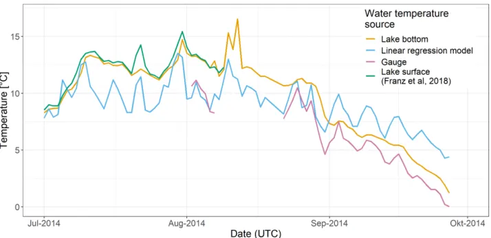
4.8 Different lake surface water temperature sources at Lucky Lake used in the aerodynamic approach model during the ice-free period in 2014 . . . 18

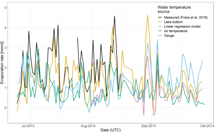
4.9 Comparison of evaporation rates at Lucky Lake during the ice free period in 2014 using different surface water temperature sources . . . 19

5.1 Measured and calculated evaporation rates for Lucky Lake during the ice free period in 2014 . . . 20

5.2 Measured and calculated evaporation rates for the ice-free periods at Lucky Lake . . 22

5.3 Water balance for Lucky Lake in 2015 . . . 23

5.4 Water balance for Lucky Lake in 2017 . . . 25

5.5 Measured and calculated water levels for Lucky Lake using different evaporation methods . . . 27

A.1 Level 1 data used for evaporation calculations . . . 41

A.2 X-y scatterplot of evaporation rates at Lucky Lake during the ice-free period in 2014 using different surface water temperature sources . . . 42

A.3 X-y scatterplot of measured and caluclated evaporation rates for Lucky Lake during the ice free period in 2014 . . . 43

A.4 Testing the aerodynamic approach with different ranges of air and water temperature and wind speeds . . . 44

A.5 Precipitation, snow-water-equivalent, change in water level, discharge and estimated evaporation during the study period from 2014 to 2017 . . . 45

List of Tables

4.1 Water balance for 25^th July to 2^nd August in 2016 . . . 14

5.1 Water balance during ice and snow free period in 2015 and 2017 . . . 26

6.1 Exemplary comparison of rainfall events between the meteorological site on Samoylov Island and rainfall measurements at Kurungnakh Island in 2015 . . . 31

A.1 Table of used symbols . . . 35

A.2 Uncertainty of water balance components . . . 36

A.3 Snow-free period on Kurungnakh and Samoylov Island . . . 37

A.4 Ice-free period at Lucky Lake on Kurungnakh Island . . . 37

A.5 Formulas and variables used for evaporation computation . . . 39

(6)

1 Introduction

Thermokarst lakes are an elementary part of permafrost affected landscapes in the Arctic; they influence geomorphologic, hydrologic and ecologic systems on different temporal and spatial scales. Permafrost, defined as ground that ”remains below 0^◦C for at least two consecutive years”

(VanEverdingen2005), underlays about 13-18% of the exposed land surface in the Northern hemisphere (Brown1997). The landscape evolution influences the distribution of thermokarst lakes and resulted in the current hydrological and geomorphological conditions (Grosse2008). On a circumpolar scale thermokarst lakes make up 20 to 50% of a permafrost area (Brown1997).

In terms of climate change, the Arctic is expected to experience rapid changes. Arctic temperatures raise twice as fast as the global mean since the last 50 years (SWIPA2017). This comes along with an observed raise in near-surface temperature of colder permafrost (0.5 to 2^◦C during the last 20 to 30 years), increased active layer depth and permafrost degradation (Biskaborn2019;

SWIPA2017; Romanovsky2010). In addition, the effects of shifting snow and rainfall regimes as well as potential increase in evaporation are still discussed in current arctic research (SWIPA2017).

The Arctic Freshwater Synthesis (Prowse2015) as well as the report of the Arctic Monitoring and Assessment Programme (AMAP) on Snow, Water, Ice and Permafrost in the Arctic (SWIPA2017) point out, that a better understanding of hydrological processes and water balances in permafrost regions is needed to understand effects on i) permafrost thaw and degradation, ii) ecological systems and iii) the biochemical cycle; especially the release of the greenhouse gases CO₂ and CH₄ from lakes and ponds. Additionally, the lifestyle of indigenous people is linked and dependent on thermokarst lakes as it supplies water and hunting space (Riordan2006; Hinkel2007; Berkes2002). Rapid water balance changes and flooding events, as observed in Alaskan and Canadian Arctic, can increase the risk to people or industries (Marsh2007).

Estimations of lake water balances are based on simple input (e.g. precipitation, inflow) and output (e.g. outflow, evaporation) calculations. Especially evaporation measurements are rare in Arctic regions and, thus, different studies estimated open water evaporation by meteorological approaches like Penman equation, Priestley-Taylor model, Blaney-Criddle method or empirical relations by Turc1954 Some of these methods are relatively data intensive, so studies came back to very simple approaches with higher uncertainties as found in Gibson1996 and Rosenberry2007 (e.g.

Chen2014; Jones2011;Turner2014; Karlsson2012; Pohl2006;Arp2011).

Remote sensing studies observe an increase in lake area for continuous permafrost in Russia and a decline in Northern America and discontinuous permafrost areas (Yoshikawa2003; Smith2005;

Nitze2018). Even though the hydrological response of Arctic landscapes and thermokarst lakes to climate change is very complex (MacDonald2016), changes in temperature and thereby permafrost degradation (e.g. Smith2005; Jones2011; Karlsson2012), changes in precipitation (e.g. Plug2008; MacDonald2012) and evaporation (Riordan2006; Bouchard2013) as well as

(7)

inevitable (Turner2010). Additionally, remote sensing needs ground truth data for validation.

Further improvement is only possible with field data (SWIPA2017; Jones2011)

Several ground based investigations in the North American Arctic has been undertaken in the past (e.g. Rovansek1996; Quinton1999; Woo2006; Pohl2006; Woo2008) whereas the Russian Arctic is rather underrepresented (see Boike2008 for the Lena Delta region and Fedorov2014for the middle part of the Lena River basin).

In 2013, the Alfred Wegener Institute (AWI) in Potsdam started field based water balance investigations at ”Lucky Lake” on Kurungnakh Island in the Lena River Delta (northeastern Siberia). A discharge gauge and a lake water level sensor were installed to measure necessary hydrological data at the lake (Niemann2014). Within this bachelor thesis, I analyse the recorded time series from 2014 to 2017. Taking meteorological data of a nearby climate station on Samoylov Island into account (Boike2019), I estimate the water balance of the lake (as it is done in Niemann2014 and Bornemann2016). Additionally, I focus on the effect of different approaches to estimate lake evaporation.

My research hypotheses are:

1. AsSmith2005 found lakes in continuous permafrost conditions to expand, the annual water balance is positive.

2. Due to relatively low snowfall during winter, the water balance is influenced by snow melt only during the early part of the open water season.

3. Water balance key driver is precipitation throughout the summer.

4. There are high differences between the three applied evaporation methods.

An introduction into the scientific topic of thermokarst lakes is given [2] before the study lake

”Lucky Lake” is introduced [3]. Field data collected on Kurungnakh Island and at Samoylov Research Station is described and used to derive the water balance of the lake. The uncertainty of every water balance component is estimated [4]. Further, results are presented and discussed [5, 6].

(8)

2 Scientific background

A main concern in hydrology is freshwater and its distribution as it is important for flora and fauna. Understanding the effects of freshwater distribution on a temporal and spatial scale is fundamental for investigating and modelling biogeochemical cycles, trapping of sediment as well as dealing with ecological and conservation concerns (Messager2016). About 2.5% of the worlds water is freshwater (Black2009) of which only 0.8% is available on the surface (Messager2016).

About 70% of freshwater are stored in glaciers, snow or ice as well as permafrost; the lasting nearly 30% is groundwater (Black2009). Regions in North American and Russian Arctic as well as Scandinavia show the highest limnicity (lake area distribution) with up to 50% land surface cover (Messager2016; Pekel2016; Brown1997). Most of these water bodies developed during the late Pleistocene-Holocene transition and the Holocene Thermal Maximum as a result of increased thermokarst in permafrost regions (Kokelj2013) covering 13-18% of the exposed land surface (Brown1997). Shallow lakes occur in these regions, having a mean depth of 2.5 to 5 m.

The term ”thermokarst” is defined as the geomorphological process by which thawing of ice-rich permafrost results in characteristic landforms. Hence, a thermokarst lake is a water filled depression developed from settlement of thawing ice-rich permafrost (VanEverdingen2005).

To understand the role of thermokarst lakes in Arctic landscapes, the genesis and development of lakes was studied in the past. Soloviev1973 gave a simple overview and description of the development of these lakes: The degradation of ice-wedges and thaw of permafrost leads to shallow depressions which fill up with water depending on precipitation and the permafrost table and water flow regime forming a broad flat basin with a lake in the middle. After the (initial) formation, the lake can undergo different changes. Lakes can coalesce with each other or (partly) drain with further permafrost degradation. Pingos and ice cored mounds can evolve at the same time (Soloviev1973). Every stage is related to different morphological characteristics and deposits. Thus, it is necessary to consider these stages in further examinations (Morgenstern2011).

Water balances of thermokarst lakes were investigated more frequently since the beginning of the 21^th century. Many studies use remote sensing data (e.g. Smith2005; Arp2011; Turner2014) because i) investigated lakes are less accessible without the necessary infrastructure, ii) larger regions can be covered more easily and iii) satellite data availability and processing has im- proved. However, isotope ratio analyses (Turner2010; MacDonald2016), direct measurements (Pohl2006) and palaeolimnic investigations (MacDonald2012) were made to overcome remote sensing disadvantages as poor short time resolution and indirect identification of reasons. Even indigenous people were interviewed to get insight of water balance dynamics (Hinkel2007).

Additionally, many of these studies use different methods to estimate lake evaporation rates based on available data and study period. For example, Pohl2006andArp2011 applied the Priestley-Taylor model to the Mackenzie Delta in Canada and Alaska resp.; the aerodynamic approach was used at Old Crown Basin in Canada and the Yukon Flats in Alaska by Labrecque2009 and Chen2014 resp.; and other more simple methods (Thornthwaite’s method, Blaney-Criddle method and the

(9)

lakes. In the past 50 years regions with discontinuous permafrost showed a decrease in lake surface area whereas lakes in continuous conditions had positive water balances. Additionally, lakes in Northern America were increasing until 1970-1990 depending on the region but then decreasing (Riordan2006; Marsh2007; Plug2008; Jones2011; Arp2011; MacDonald2012;

Bouchard2013; Turner2014), under some conditions in catastrophic events (Pohl2006;

Labrecque2009; Jones2015) even if observation of rapid lake drainage and the exact timing remains difficult with remote sensing data (Labrecque2009). Jones2011 also found the total number of lakes increasing whereas the surface area declines. They explained this observation with draining lakes leaving remnant ponds. Different studies tried to figure out potential key drivers for the observed change in water balance; they can be summarised into three main reasons.

1. Rising temperature and linked permafrost degradation was suggested to be one reason (Smith2005; Marsh2007; Jones2011; Roach2011; Karlsson2012). Two contrarious processes are described. Permafrost degraded at lake margins resulting in mass movements into the lake increasing the surface area (Jones2011). Degradation of the permafrost table created new drainage ways leading to greater outflow and decline of the lake (Smith2005). Especially increasing active layer thickness in combination with high water levels results in increasing lake drainage as the lake bank becomes more unstable (Marsh2007).

2. Climate change did not only affect the temperature of permafrost but also the local distribution of precipitation and evaporation which is suggested as another reason for change in lake extend (Plug2008;Riordan2006; MacDonald2012; Bouchard2013). The ratio of precipitation and evaporation can change because of locally shifting snow- and rainfall patterns as well as a climate driven rise in evaporation. The combination of these processes can result in negative and positive water balances (Riordan2006; Plug2008; Bouchard2013). In addition, increasing rainfall during summer month can lead to more surface and subsurface drainage (MacDonald2012).

3. Considering a combination of different reasons can explain observed changes as well.

Pohl2006 suggested a combination of summer temperature, precipitation and lake water level;

Labrecque2009found the general change in climate conditions as main reasons;Arp2011found drying lake in Alaska due to permafrost degradation and increased evaporation;Turner2014sug- gested the seasonal change in precipitation and the change in vegetation coverage as key drivers and Fedorov2014considered next to permafrost degradation also the anthropogenic impact.

However, hydrological responses of lakes and ponds in the arctic remain a very complex question at the local scale (MacDonald2016). In addition, many findings are based on studies in North American Arctic, but the Russian Arctic remained mostly unconsidered in the past.

Based on the findings described above and own isotope studies, Turner2010 suggests a lake classification based on hydrological processes influencing the water balance. They found different key drivers of the short term water balance for lakes in the Old Crown Flats (Yukon Terri- tory in Canada) and named each class accordingly: ”snowmelt-dominated, rainfall-dominated, groundwater-influenced, evaporation-dominated and drained” (Turner2010). They also described the occurrence of each type and its main characteristics. Snowmelt-dominated lakes occurred in landscapes characterised by higher and more dense vegetation, whereas rainfall-dominated were found in low tundra vegetation. Through the summer, snowmelt-dominated lakes became rainfall- dominated as the influence of melt water decreased. Lakes in floodplains were mainly ground-water dominated as river water represented an additional subsurface input source. Evaporation-dominated lakes occurred in drier areas and are more vulnerable to future changes in temperature or rainfall distribution as they may drain completely (Turner2010).

(10)

The greatest interest in investigating water balances of thermokarst lakes lies, next to catastrophic drainage events, in determining the effect of lakes and ponds on carbon release to the atmosphere.

Permafrost degradation causes influx of (old) organic carbon into water bodies which is then de- composed to carbon dioxide (CO2) or methane (CH4) and released to the atmosphere. There it acts as a greenhouse gas which enhances global warming leading to further degradation and forcing the positive feedback to intensify (Schuur2008). It is still difficult to asses the amount of carbon released from lakes and ponds, but progress is made since the last 15 years. Walter2006was one of the first to describe lakes as major carbon source. Due to a new, continuous measurement method, they found emissions to be five times higher than previously estimated (3.8 Tg per year for North Siberian lakes). The amount of greenhouse gas released from any water body to the atmosphere can vary spatially and temporally. For large lakes, the margins are found to have higher emission rates (Walter2006), whereas small ponds show higher emissions for open water zones (Abnizova2012).

Dynamics of the mixed layer influence the release on a daily scale, whereas the overturn in autumn is important on a seasonal scale (Laurion2010; Abnizova2012). During the freezing period in autumn, methane is produced because of missing oxygen and is stored in bubbles in the ice cover of lakes and ponds until it gets released in spring (WalterAnthony2013;Langer2015). Additionally, it was found that local hydrology (e.g. water level or the amount of soil moisture) is one of the key controls on methane emissions in tundra landscapes (Olefeldt2013). Thus, Abnizova2012 con- cluded, that carbon emission models tend to underestimate the amount of released carbon resulting in conservative future temperature projections.

(11)

3 Study area - ”Lucky Lake” on Kurungnakh Island

The Lena River Delta (72^◦N, 126^◦E) represents the last part of the 4400 km long Lena River, having its source near Lake Baikal and flowing up into the Laptev Sea, Arctic Ocean. About 30 km³ of water flows through the delta every year showing an increasing trend since 1977 (Fedorova2013).

The delta covers an area of about 25 000 km², including more than 1500 islands with about 60000 lakes (Antonov1967). The whole delta is underlain with continuous permafrost (Brown1997).

First geological investigations described three main terraces:The first terrace, developed during the Holocene, exhibits tundra with ice wedge polygonal structure, large thermokarst lakes and active flood plains covering the central and eastern part of the delta. The second terrace (northwestern part of the delta) formed during the late Pleistocene to early Holocene and show low ice, sandy sediments with large thermokarst lakes. The third terrace developed during the late Pleistocene and is therefore the oldest terrace. Sediments are fine grained, organic and ice rich which results in polygonal surface structures and strongly expressed thermokarst processes. The eastern part of the delta, including Kurungnakh Island, is characterised by this terrace (Grigoriev1993).

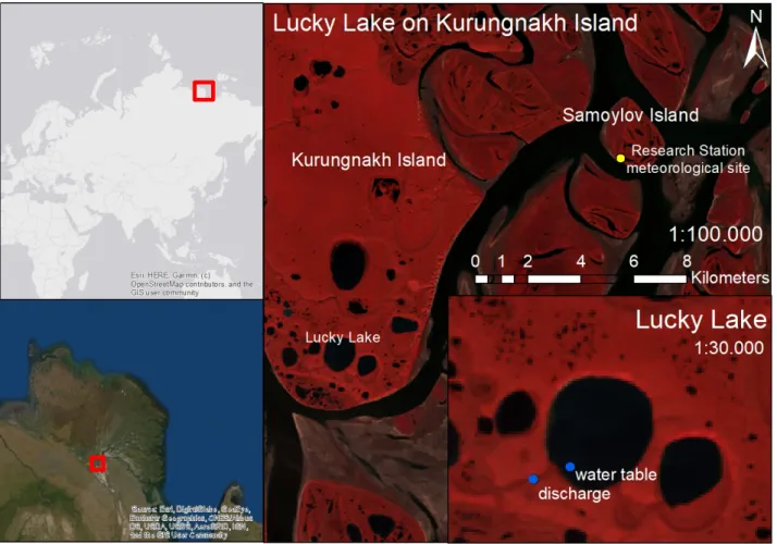
Figure 3.1: Overview map of study region and position of measurement sites

image sources (top left to bottom right): Esri, HERE, Garmin, OpenStreetMap contributors, andc the GIS User Community; Esri, DigitalGlobe, GeoEye, Earthstar Geographics, CNES/Airbus DS, USDA, USGS, AeroGRID, IGN, and the GIS User Community; color infrared image, Landsat 8, 28.6.2018

(12)

On Samoylov Island, central part of the Lena River Delta, a research station was installed measuring meteorological data since 1998 (Figure 3.1). The average annual air temperature was−12.3^◦C with the warmest month in July (9.5^◦C) and the coldest month in February (−32.7^◦C). The average annual rainfall was 169 mm (Boike2019).

About 2 km to the east of Samoylov Island, the far bigger Kurungnakh Island is located (72^◦19’N;

126^◦12’E, 350 km²; Figure 3.1). About one third of the surface area is affected by thermokarst processes. Morgenstern2011 suggests that for thermokarst investigations, a differentiation between lakes on Yedoma (very ice- and organic-rich sediment) upland and lakes in thermokarst basins is useful. They also found that lakes on the Yedoma upland have a higher potential to release carbon and are more sensitive to climate change.

The investigated lake, Lucky Lake, is located in the south of Kurungnakh Island (about 10 km from Samoylov Island) on the Yedoma upland (Map 3.1). The lake has an surface area of 1.22 km² and a volume of about 3.8 Mio. m³. The shallow lake has a mean depth of 3.1 m and maximal depth of 6.5 m. During winter, the lake does not freeze to the ground and is therefore characterised as a floating ice lake (Franz2018).

Since 2013, several studies focused on Lucky Lake. Firstly, the summer water balance for August 2013 was estimated. Precipitation and evaporation were found to be the main components of the water balance. The water balance for this month was negative due to more evaporation than rainfall (Niemann2014). The time series was continued and a first water balance for a whole year (2014- 2015) was presented at the International Conference on Permafrost in Potsdam 2016. Main results were a positive water balance throughout the year except the summer period where high evaporation rates dominated the water balance (Bornemann2016). In 2014, a raft with several sensors, including radiation and eddy covariance flux measurement, was installed to study the energy balance during frozen, break-up and ice-free conditions (Franz2018). These measurements underline the importance of lakes in the energy budget of a landscape. Additonally, condensation was observed during the melting season.

(13)

4 Methods and data

The water balance gives insight into the very basic hydrological characteristics of a region (Figure 4.1). It influences other geomorphological and biogeochemical processes as well as soil development and vegetation cover. Especially the influence of thermokarst lakes on carbon release is of interest in permafrost research (described in [2]).

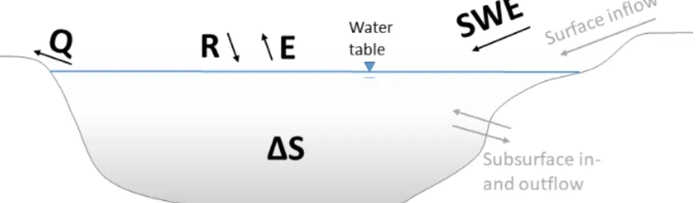
For Lucky Lake, the following water balance equation is applied (according to Turner2010):

∆S =R+SW E−(E+Q) (1)

The considered components of the water balance are rainfall (R) and snow water equivalent from snow melt (SW E) as input variables and evaporation (E) and discharge (Q) as output. Thus, the change in lake water storage (∆S) can be positive or negative. The product of difference in water level and lake area gives the change in lake water storage. Rainfall, discharge and the water level is measured directly in the field, whereas snow water equivalent and evaporation is calculated from meteorological data. Subsurface in- and outflow as well as surface inflow is neglected, because Niemann2014measured a subsurface inflow of 0 mm into the lake or simply no data are available.

Figure 4.1: Conceptual water balance of a lake (according toTurner2010); considered components are presented in black whereas unconsidered parameters are gray

R - rainfall, E - evaporation, Q - surface discharge, ∆S - change in lake heat storage

General meteorological data is derived from Boike2019. Rainfall, snow depth and necessary data for evaporation calculation are measured at Samoylov Research Station. To ensure good data quality, the instruments were checked and calibrated regularly. Further, the data was filtered automatically to detect a.o. system errors, physical limits of instruments or equipment maintenance periods as well as manually to flag visual outliers. This processing leads to level 1 data and was already done by the authors (Boike2019). For this thesis, I applied a comparable processing from raw to level 0 and level 1 data for the hydrological variables (discharge, water level and lake bottom temperature) that were directly measured at Lucky Lake (see Figure 3.1).

Raw data is read out in the field containing gaps, unequal timesteps and the measured physical variable. For processing to level 0 data, I brought data in equal time steps and filled the gaps with ”NA” for ”not available”. For discharge and water table measurements, the actual needed parameter had to be calculated from the physical variable measured in the field. Details are described in each section. Level 0 data contains every measured and calculated parameter. To bring data to the final level 1, the data was ”flagged”, meaning to add a number for each value giving information about the quality. Whereas ”0” means good data, values from 1 to 6 are used to express no data, system errors, maintainance periods, physical limits, gradient conspicuity and plausibility. The two additional flags 7 (decreased accuracy) and 8 (snow covered) fromBoike2019

(14)

are not used in this study. The flag 6 (plausibility) was evaluated visually. All flagged values (1 to 6) were removed before they were used in the model caluclations.

Additionally, measured evaporation and a water temperature profile for the ice-free period at Lucky Lake in 2014 is derived from Franz2018 These rare measurements are taken to compare the calculated evaporation rates with field data and to derive the uncertainty of the method.

Figure A.5 represents the entire dataset available for water balance calculations. A daily time scale is chosen for the water balance calculations. Snow free periods are estimated with the help of time lapse camera pictures at Samoylov Research Station (whole period) and at the discharge gauge (until 2016) in this study. Condition when water can run freely through the gauge was chosen as the start of the snow-free period. I used lake bottom temperature data (in about 2.5 m depth, depending on the water level) to evaluate the starting and ending of the ice free period at Lucky Lake (following Boike2015). In spring, lake bottom temperature raises with increasing air temperature. When the ice ”breaks up”, lake bottom temperature raises abruptly - this date was chosen as the beginning of the ice-free period. In autumn, the temperature of the whole lake drops down to about 0 to 1^◦C, before 4^◦C is reached at the lake bottom. In addition, the near-freezing date marks the end of the ice-free period. When lake bottom temperature was missing, satellite data from NASA’s EOSDIS campaign (https://worldview.earthdata.nasa.gov) and Sentinel-2 images from the Copernicus mission (ESA, https://apps.sentinel-hub.com/sentinel-playground/) was used to estimate the ice-free period for data gaps in September 2015, June 2016 ans September 2017 in this thesis. Snow- and ice-free periods are presented in Table A.3 and A.4.

The uncertainty laying in hydrological studies is still of interest in hydrological research, for which an ”Uncertainty Assessment in Surface and Subsurface Hydrology” was elaborated in 2005 to 2009 (Montanari2009). Some dynamics of processes are not understood so far and together with problems in geometric representation (e.g. lake bathymetry or river cross-section) and little available data, every hydrological study includes uncertainties which must be considered in modelling and communicated for a better understanding of results. Four main reasons for uncertainty were figured out: i) randomness of the variable, ii) model structure error, iii) errors in parameter value and vi) data error (Montanari2009). Within this study, the uncertainty (σ) of every component was assessed by combining instrument accuracy, uncertainty values from literature and calculated uncertainties (see Table A.2 for a summary). The overall uncertainty of the water balance is computed according to error propagation. Absolute errors (∆x =x∗σ_x, x meaning any water balance component) are summed up for addition and subtraction terms:

∆S_min =R∗(−σ_R) +SW E∗(−σ_{SW E})−(E∗(+σ_E) +Q∗(+σ_Q)) (2) and

∆Smax =R∗(+σR) +SW E∗(+σSW E)−(E∗(−σE) +Q∗(−σQ)) (3)

(15)

4.1 Rainfall

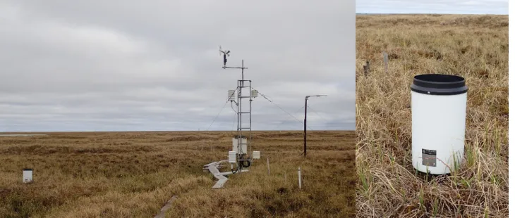
Rainfall was measured half-hourly by a tipping bucket raingauge (52203 Young Tipping Raingauge by Campbell Scientific) installed on Samoylov Island (Figure 4.2). A height of 0.35 m was chosen to prevent snow cover and to reduce wind influence (Boike2019). The tipping bucket raingauge collects rainfall water in a small bucket similar to a seesaw. After a certain amount of water is collected (0.1 mm for this raingauge), the container tips to the other side and empties the water into a greater container. The number of tips can be counted electronically and easily computed into the amount of rainwater. Tipping bucket raingauges tend to underestimate rainfall, but they record the intensity (amount of water per time unit) and are therefore useful for remote areas.

Figure 4.2: Left: meteorological station on Samoylov Island; right: tipping bucket gauge for rainfall measurements. Photos by P. Schreiber

The measurement of rainfall is susceptible to different error sources. The main uncertainty is due to wind speed (e.d. WMO2008; McMillan2012 and Yang1998). McMillan2012 gives an uncertainty of 10% for an average wind speed of 6^m_s based on a literature survey whereas Yang1998 developed catch ratio equations for different precipitation conditions and wind shields. Applying their equation to the rain gauge at Samoylov Research Station [A.4], an uncertainty of 9.4% is calculated for an average wind speed of 4.4^m_s.

Other error sources can come from evaporation of the collected water (WMO2008; Yang1998), and the influence of snow drift into the gauge system (WMO2008). Due to little snow cover during winter, the error caused by solid precipitation is rather low. Uncertainty due to evaporation is neglected here because the number of tips is measured and not the amount of water over a certain period. Evaporation acts on a greater temporal scale than the measurement device.

The manufacturer gives an measurement accuracy of 2% for rainfall intensities below 25^mm_h . This intensity was not exceeded during the study period. It is not clear if wetting loss and the speed at which the bucket tipping mechanism works is already considered in the accuracy of the manufacturer. They are not regarded specifically here, because these errors are relative low compared to wind, evaporation and snow influence.

Taking all these error sources together, I evaluated an uncertainty of 12% for the rainfall measurement at Samoylov Research Station. Still not considered is the distance between Samoylov Island and Lucky Lake on Kurungnakh (about 10 km), which lays in the scale of variability (Adam2003).

(16)

4.2 Snow melt

Water from snow melt is included in the water balance equation as block input at the last day of the snow covered period. There is no direct measurements of snow water equivalent (SWE [mm]) at Samoylov or Kurungnakh Island, so a simple calculation approach was chosen:

SW E = d_s∗ρ_s ρw

(4) d_smeans snow depth (highest value of the continuously half-hourly measured time series on Samoylov Island for each winter, [m], Boike2019), ρ_s means snow density [_m^kg3], and ρ_w means density of water (= 997_m^kg3). Average, minimum and maximum snow densities (195, 175 and 225_m^kg3, resp.) are derived from Boike2013. Snow characteristics were investigated during winter 2008, but the measurements are suitable for a rough estimate.

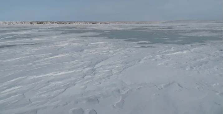
The measurement of snow depth at the Samoylov site is very precise with 0.4% accuracy given by the manufacturer (Boike2019). The greatest error source is snow drift which can only be observed locally. This means the the temporal and spatail variability affects the uncertainty more than the actual measurement accuracy. Observations at Lucky Lake show a more or less snow-free ice surface with local snow accumulations at the margins (Figure 4.3). The drift of snow within the catchment will affect the amount of melt water inflow as well.

It is quite difficult to estimate the actual uncertainty of snow melt water input. Thus, the range of minimum and maximum snow densities are chosen as uncertainty boundary values.

Figure 4.3: Snow conditions at Lucky Lake in April 2019. Photo by F. Tautz

(17)

4.3 Discharge

Discharge is measured at the outlet channel in the south-west of the lake every 10 s by the RBC flume 13.17.08 of Eijkelkamp (Figure 4.4 and Map 3.1). Water level in the gauge is measured by a radar sensor (VEGA-Puls WL 61), from which discharge can be calculated according to the rating equation given by the manufacturer [A.5]. Operating range of the equation is given with 2 to 145_s^l. In 2017, this equation had to be extrapolated until a rate of 180^l_s because of high outflow due to snow melt. Data was filtered accordingly to the measured water temperature (temperature>0^◦C as ice blocks the gauge so that water cannot run freely through the weir) as well as visually to leave out outliers. To get the actual output in mm, the measured discharge rate has to be divided by the lake area (derived from a bathymetric map) and adjusted to the daily time scale.

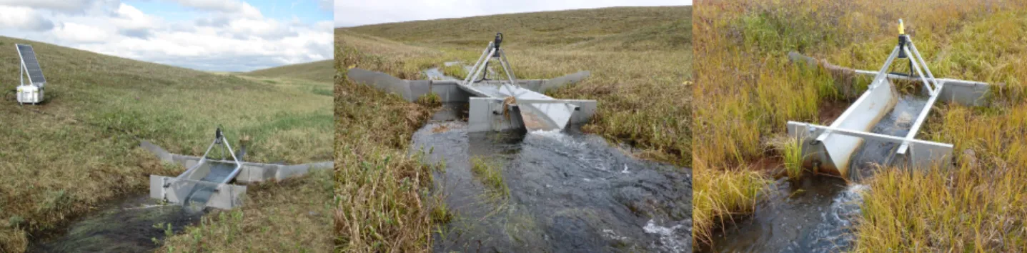
Figure 4.4: left: discharge gauge after installation in 2013. Photo by N. Bornemann; center: high discharge rates after snow melt in 2015. Photo by P. Schreiber; right: gauge in summer 2017. Photo by N. Bornemann

A time lapse camera was installed in the valley from 24.4.2014 until 1.12.2016 providing daily images of the gauge. In this study, pictures were used to define the start and end of the discharge time series for every year. During winter, the gauge is (completely) covered with snow which, when melting, floods parts of the valley. The beginning of the time series was defined when water starts to run freely through the channel. The first frost defined the end of the time series every year. Data before and after these defined dates is left out which unfavourably leads to a lack of data in the first part of the snow free season (Figure A.5).

Although a gauge with a known cross-section is already a very reliable method for discharge measurements (Harmel2006), there are still some error sources: i) an average uncertainty of 5 to 10%

is inherent to every discharge measurement using a gauge (Harmel2006); ii) the extrapolation of the rating equation adds uncertainty which was found to be up to 6% as an average value from different studies (McMillan2012); iii) the error due to the bathymetric map from which lake area was derived cannot be reconstructed here; iv) the manufacturer of the radar sensor gives an measurement accuracy of ±2 mm.

Even if some uncertainties can be quantified very well and others remain more qualitative, an overall uncertainty of 16% can be assumed. Especially high discharge rates during spring (Figure 4.5) must be considered more uncertain.

(18)

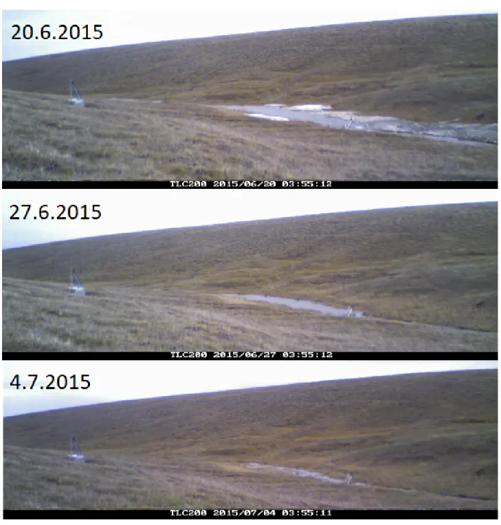
Figure 4.5: Example of spring flooding at the gauge during snow melt from 20.6.2015 until 4.7.2015;

discharge time series in 2015 started on July 6^th; photos derived from time lapse camera

(19)

4.4 Change in lake water storage

Change in lake water storage can be observed by the change in its water level. Thus, a pressure sensor (HOBO U20-001-01-Ti by Onset) was installed at Lucky Lake measuring hourly hydrostatic pressure and bottom water temperature in about 2.5 m depth, depending on the water level (Map 3.1). Changes in water level due to data read-out and installment of a new senor were filtered.

Additionally, the data is air pressure corrected in this study (for processing details, see [A.6]).

Data is available from 22.8.2014 to 12.9.2015 and 22.7.2016 to 15.9.2017. Thus, there is no information about the freeze in 2015 and break up in 2016. A discontinuous water level time series makes it difficult to plot water level as absolute values and a relative scale is chosen.

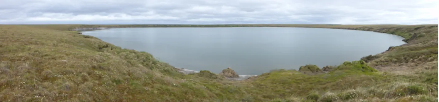
Figure 4.6: Lucky Lake on Kurungnakh Island in summer 2016. Photo by N. Bornemann

A decrease of 30 cm in water level within 3h was measured starting at 17pm on the 1^st of August 2016. After excluding that any person moved the sensor at this time, there can be different reasons:

i) movement of the sensor by ice or wind influence, ii) water balance, e.g. increased discharge, iii) drainage through the valley with the gauge but not measured (another unknown flow path) vi) break through of the bank resulting in a rapid drainage into another valley and vi) measurement error of the water level sensor. The first reason is quite unlikely because the lake was already ice-free and moderate to high wind speeds were measured (9.1^m_s at highest; 1^st of August at 18pm). Table 4.1 presents a rough water balance calculation and does not explain the high loss in water storage.

Returning to Lucky Lake in 2017, no obvious change of the lake or the discharge channel bank was observed, but these reasons cannot be excluded. In addition, Morgenstern2011 suggests rapid lake drainge as unlikely as the lake is located on the Yedoma upland. In the following, the value is seen as a measurement error and left out in further calculation.

Table 4.1: Water balance for 25^th July to 2^nd August in 2016

E was estimated by summing the average evaporation rate of 1.2^mm_d [5] during the eight days water balance component amount of water [mm]

R 22

Q - 22.7

E - 9.6

calculated ∆S -10.3

measured∆S - 301.6

Water level can be measured very precisely - the manufacturer gives a measurement accuracy of 0.1%. When it comes to estimate the absolute value of lake water storage, the uncertainty of the bathymetric map would add the greatest error (Winter1981). Here, the relative change in water level is considered and therefore the influence of bathymetry reduced.

Overall, an uncertainty of 5% is estimated for the water level measurement.

(20)

4.5 Evaporation

The process of evaporation describes the transition of open water from liquid (e.g. rivers and lakes) to gaseous (water vapour in the atmosphere). It links mass and energy flux of a landscape:

E = Q_E

L_v·ρ_a (5)

with evaporation E as flux of mass,Q_E as energy flux, L_v as latent heat of vaporisation andρ_a as air density.

In hydrology, it is common practice to use meteorological data to estimate evaporation rates. Several approaches were developed in the past using different variables (e.g. air temperature, humidity, wind speed, days of sunshine) with different temporal resolutions (yearly to hourly average). Due to the good data availability with high temporal resolution at Lucky Lake, the Penman equation (also known as Combination Model) and the Priestley-Taylor model are chosen to estimate evaporation in this study. Both approaches have been used for Arctic lakes in other studies (Stewart1976;

Marsh1988; Gibson1996; Marsh2007; Arp2011). Additionally, an aerodynamic approach from a physical boundary layer perspective is applied (Oke1978; Garratt1994). Evaporation rates are calculated daily for the ice-free period in this thesis (Table A.4).

In the following three sections, the general idea of each evaporation model is presented as well as the main equations. Computation details can be found in [A.7]. Figure A.1 shows input data for the evaporation models measured at Samoylov Island and Lucky Lake.

The calculated evaporation rates are compared to measured time series data byFranz2018. Beside other parameters relevant for the energy balance, they also measured hourly evaporation rates using an eddy covariance flux system directly located on a floating lake platform. The standard error deviation is used to estimate the uncertainty of every method [4.5.4].

4.5.1 Penman equation

Penman1948showed that a combination of mass and energy flux is suitable for deriving evaporation rates for open water conditions. He adjusted the model with an empirical term according to a lake in Rothamsted (United Kingdom) to verify the approach. About 20 years later, VanBavel1966 replaced this empirical term with a wind function so that the combination model can be applied to general open water conditions. The Penman equation is often used as the ”standard” method to estimate evaporation rates (E) in hydrology:

E = ∆·R_net+γ·K_E ·ρ_w·L_v·u_z₂ ·E_sat_z

2 ·(1−RH_z₂)

ρ_w·L_v ·(∆ +γ) (6)

where ∆ is the slope of the saturation vapour pressure curve [^kPa◦C], R_net is net radiation [^W_m²], γ means psychrometric constant [^kPa◦C], K_E is water vapour transfer coefficient [_{d m kPa}^{mm s} ] (dependent on lake area), ρ_w is water density (= 997_m^kg3), L_v is latent heat of vaporisation [^MJ_kg],u_z₂ is wind speed

(21)

4.5.2 Priestley-Taylor model

Based on the Penman equation, the Priestley-Taylor model was developed. The main assumption is that the mass balance term can be neglected because air becomes saturated when it is transported over well-saturated land for long distances. This simplified Penman equation was called equilibrium potential evapotranspiration (Slayter1961). Priestley1972 investigated this assumption in the field for different surface conditions and found a close fit between measured and modelled evaporation by adding a factor α:

Q_E =α· ∆

∆·γ ·(R_net−G) (7)

where ∆ means the slope of the saturated vapour pressure curve, γ means the psychrometric constant, R_net means net radiation and G means subsurface heat flow. α was found to be 1.26 by different studies, e.g. Priestley1972 and Stewart1976.

Equation 7 has to be inserted into Equation 5 to get the evaporation rate in ^mm_d .

Subsurface heat flow can be estimated by adding change in lake heat storage (G_W) and heat conduction into the lake bed (G_B):

G=G_W +G_B (8)

Heat conduction into the lake bed was neglected here, as it was found to be zero in other studies over an annual study period (Marsh1988; Rosenberry2007 and Arp2011). The change in lake heat storage G_W can be estimated using the following equation:

G_W = c_w·T_w·ρ_w·d

∆t (9)

with c_w is specific heat capacity of water (= 4.81_{g K}^J ), T_w is change in water temperature over a time step ∆t (= one day),ρ_w is water density (= 997_m^kg3) and dmeans mean lake depth (= 3.1 m).

4.5.3 Aerodynamic approach

Beside both meteorological approaches to estimate evaporation, a third approach from a physical boundary layers perspective is applied. A gradient between the water surface and two meters height is used to calculate the energy difference which is balanced by the evaporation process (Figure 4.7).

The approach is generally described inGarratt1994and applied to arctic ponds on Samoylov Island byMuster2012. According to their description, the approach was computed:

QE = −L_v·ρ_a

r_a ·∆u·∆pV (10)

whereQE means energy flux,Lv means latent heat of vaporisation,ρa means air density,∆umeans the difference in wind speed and ∆p_V means the difference in vapour density between both heights (∆u = u_z₂ −u_z₀ resp. ∆p_V = p_V_z

2 −p_V_z

0). The aerodynamic resistance r_a is described further below (Equation 11). Wind speed at water surface height is assumed to be 0^m_s and relative humidity is set to be 100% (Figure 4.7). Using Equation 5, the evaporation rate can be derived in mass units.

(22)

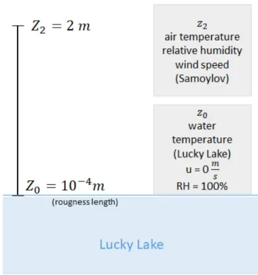
Figure 4.7: Schematic overview of aerodynamic approach and parameters

∆p_V gives the gradient that has to be balanced whereas ∆u describes the amount of air movement.

The higher the wind speed, the more humid air gets transported and thus, the gradient keeps upright and more evaporation can occur (Figure A.4).

The aerodynamic resistance can be calculated as follows:

r_a= ln(^z_z²

0)²

k²∗u_z₂ (11)

where z₂ is the measurement height (2 m), z₀ is the roughness length (10^-4 m for calm surface conditions; Garratt1994), k is the Karaman’s constant (= 0.4) and u_z₂ means the wind speed at measurement height. Wind speed was measured at three meters height but two meters height is required for the model. Due to low tundra vegetation and the exponential curve of wind speed with height, wind speed at both heights is assumed to be the same.

This approach needs very local high quality data (Winter1981) of water surface temperature, humidity and wind speed which limits the practice of the model. Here, data from Samoylov Research Station (air temperature, humidity, wind speed) and Lucky Lake (water temperature) are combined.

Water temperature at lake bottom (in about 2.5 m depth, depending on the water level) was measured by the pressure sensor also used for water level measurements. Figure 4.8 shows similar development of lake bottom and surface temperature. Additionally, lake water was found to cir-

(23)

ture was assumed to be the same as water temperature. Boike2015 found a strong 1:1 correlation between monthly air and lake temperature during summer. This relation also exists on a daily basis even if it is not as expressed as for monthly values. And third, a linear regression model based on daily water and air temperatures was set up. Water temperature sources and evaporation rates for different temperatures are presented in Figure 4.8 and 4.9.

Figure 4.8: Different lake surface water temperature sources at Lucky Lake used in the aerodynamic approach model during the ice-free period in 2014; Lake bottom temperature was measured in about 2 m depth, depending on the water level. The linear regression model is based on a daily relationship between air and lake bottom water temperature. The gauge is in 200 m distance to the lake outflow.

Generally, the difference between measured and calculated evaporation is small. Calculated evaporation from different temperature sources follow the same general dynamic. The approaches using air and modelled temperature tend to underestimate the absolute evaporation value, whereas bottom temperature under- resp. overestimates low resp. high values. Because of the little overlap between temperature data of the gauge and measured evaporation rates, the quality of the method cannot be assessed. Over the whole study period from 2014 to 2017, models using this temperature generates more condensation (negative value) compared to the others - especially in the period of data lack.

Finally, the data gap was filled with implemented data from the linear regression model, because it fits measured evaporation the best with regard to absolute values and overall dynamics.

(24)

Figure 4.9: Comparison of evaporation rates at Lucky Lake during the ice free period in 2014 using different surface water temperature sources; A x-y scatterplot is included in the appendix (Figure A.2).

Evaporation was measured by an eddy covariance flux system located on a floating raft at Lucky Lake (Franz2018). Lake bottom temperature was measured in about 2 m depth, depending on the water level. The linear regression model is based on daily air and lake bottom water temperature. The gauge is within 200 m distance to the lake outflow.

4.5.4 Uncertainty

The uncertainty of evaporation models is difficult to assess, because randomness of the natu- ral process, measurement uncertainty and model structure error have to be taken into account (Montanari2009). The randomness of evaporation cannot be assessed here. As eddy covariance flux measurements are a very precise technique (Winter1981), the measured values are assumed to be not uncertain in this study. Based on that, standard error deviation (p=0.95) is used to derive the uncertainty of each method [A.8]. This calculation does not consider the uncertainty of any input data into the model.

Following uncertainties are obtained:

• Penman equation: 37%

• Priestley-Taylor model: 55%

(25)

5 Results

5.1 Evaporation

In this study, evaporation was calculated using three different approaches [4.5]. A comparison with measured data for the ice-free period in 2014 (Franz2018) is shown in Figure 5.1. Evaporation measurements by a eddy covariance flux system located at a floating raft on the study lake are very rare and exceptional data. So far, no other evaporation measurements were successfully undertaken at the lake, so this is the only period for which a comparison to modelled values is possible.

Figure 5.1: Measured and calculated evaporation rates for Lucky Lake during the ice free period in 2014; A x-y scatterplot is included in the appendix (Figure A.3). Measurements were done by an eddy covariance flux system on a floating raft at the lake (Franz2018). The three evaporation models are described in [4.5].

(26)

The Penman equation and the aerodynamic approach follow the general alteration of the measured evaporation with the aerodynamic approach doing this more closely. High and low values are little over- resp. underestimates by the aerodynamic approach, whereas the Penman equation underestimates evaporation rates in most cases. The Priestley-Taylor model shows an opposing trend to the measured values especially in the beginning of July and in mid-August. Additionally, this model estimated too high and too low values - for some days up to five times higher than the measured evaporation.

Evaporation rates for the whole study period from 2014 to 2017 can be found in Figure 5.2. Overall, all three methods give relative constant values without a temporal dynamic throughout the year. There only is a slight decrease in evaporation for the Priestley-Taylor model during the ice-free period.

Results from the Penman equation range relatively constant around an average of 0.4^mm_d and no condensation is predicted. The mean evaporation rate from the Priestley-Taylor model is calculated to be 1.4^mm_d , with a range of −7 to 10^mm_d . The highest and lowest values are very questionable.

Additionally, great changes within a day are computed especially in the beginning of the ice-free period. These great changes occur when water temperature and therewith lake heat storage changes. A negative change in lake heat storage results in latent heat release which gets balanced by cooling and possibly condensation (e.g. 12.8.2014 and 18.7.2016). The aerodynamic approach ranges within little condensation (−2.5^mm_d at lowest) and high evaporation (up to 5^mm_d ). High evaporation rates always occur with high wind speeds (e.g. 30.8.2014, end of September 2015, 3.8.2017). Condensation is predicted shortly after ice-break up when water temperature is still low but air temperature increases rapidly (e.g. end of June 2017) and on very warm mid-summer days when the gradient between water and air temperature gets the highest (e.g. 8.8.2015, 2.9.2016 and 7.8.2017; see also Figure A.4). The mean evaporation rate for the aerodynamic approach is 1.2^mm_d . Summarised, the Penman equation gives the smallest values with little variability and the Priestley- Taylor models the greatest values with big variability. The Penman equation and aerodynamic approach follow the same dynamic. The Priestley-Taylor model shows an opposing trend as compared to the other two methods.

Key findings

• The aerodynamic approach shows the closest fit to measured data from eddy covariance flux measurements located on a floating raft at the lake (Franz2018). Average evaporation rate is 1.2^mm_d using the aerodynamic approach.

• The Penman equation and the aerodynamic approach follow the same dynamic as measured evaporation rates. Contrary, the Priestley-Taylor model shows an opposing trend.

• The Priestley-Taylor model and the aerodynamic approach predict condensation to occur.

(27)

Figure 5.2: Measured and calculated evaporation rates for the ice-free periods at Lucky Lake; Measure- ments were done by an eddy covariance flux system on a floating raft at the lake (Franz2018). The three evaporation models are described in [4.5].

(28)

5.2 Water balance

As found in [5.1], the aerodynamic approach shows the closest fit to measured evaporation and is therefore used in the water balance calculations. During summer 2014 and 2016 either discharge recording (starting 2.8.2014) or water level measurements (lacking until 22.7.2016, see Figure A.5) limit the interpretation of the summer water balance. Thus, water balances for the years 2015 and 2017 are represented in Figures 5.3 and 5.4 using the aerodynamic approach model to estimate evaporation output. Table 5.1 shows the summed water balance components as well as the calculated change in lake water storage and compares it to the measured water level change in 2015 and 2017. The influence of evaporation models on calculated water balances is presented in Figure 5.5.

Water balance 2015

(29)

In 2015, the snow melt input into the lake is overestimated by about one third (SWE, beginning of June, Figure 5.3). Whereas 60.7 mm were calculated, 38.0 mm can be estimated from the water level change. The declining water level in the end of June is not represented by the water balance model because suitable discharge measurements start after the melt water runoff.

The calculated water level starts declining exactly at the time when the discharge measurements start because the overall output (E plus Q) is larger than the input (R). On the contrary, the measured water level steeply declines earlier and only shows a very slight decline throughout the summer, indicating only a little more output than input (Figure 5.3).

Whereas rainfall events do not turn out clearly in the measured water level change during July and August, they slightly show up in the modelled water balance. Only the last greater rainfall event (35.7 mm within five days) is represented in the measured water level change (+60.6 mm in the same five days) and in the calculated water level change but not to the same amount (two peaks in the five days, +10.0 mm and +11.2 mm). Whereas the measured water level increases in two steps, the calculated water level shows two peaks, indicating too little input or too high discharge.

After the rainfall event, the measured water level stays constant at the new level, which would suggest the rainfall event to not discharge but to be stored in the lake. Contrary, the discharge curve (Figure A.5) shows a significant increase at the same time of the rainfall event which also can be seen in the lower change in modelled water storage.

The overall summer water balance (until the end of the measured water level time series) and the model results do not fit. The end-summer water balance value is not even included in the uncertainty range of the model (Table 5.1). Water output is too high through the summer which results in differently measured and calculated dynamics and different seasonal water balances. This stronly indicates the hydrological processes to be not completely represented in the model. Accordingly to the model, discharge is the main water balance driver which cannot be confirmed from the actual development of the water level. Input and output seem to balance each other most of the time.

Water balance 2017

In 2017 (a very snow rich year), the input due to snow melt is again overestimated by nearly one third (SWE in mid-June, Figure 5.4). 129.6 mm is the calculated snow melt input but only 90.9 mm can be estimated from the measured water level change. The discharge time series starts a few days after melt water input, and results in a good representation of water level change as compared to the the measured data. The first great change right after the start of the snow free period is left out by the model, but the second peak and following decline is modelled well. This clearly underlines the need of an early start of the discharge curve.

Furthermore, the following decline in measured water level is followed well by the model until mid-August. The rainfall events turn out in the measured as well as in the modelled water level but to different amounts in the first half of the summer. The change in measured water level always exceedes the rainfall input, and, thus, the modelled water balance. Exemplary, the actual input due to rainfall was 17.9 mm in the period from 29.6.2017 to 1.7.2017, the change in measured water level was +34.4 mm, and the modelled water balance was +10.0 mm.

From 10.8.2017 to 13.8.2018 and from 4.9.2017 to 10.9.2017, one can observe two rapid rises in measured water level. Whereas for mid-August an increase of +102.2 mm in water level is measured, rainfall was only 16.8 mm. This event can be identified in the modelled water balance (+6.0 mm). The second increase in September cannot be explained by the water balance (R:

3.8 mm; measured ∆S: +109.8 mm; calculated ∆S: -10.9 mm resp.). Overall, the input amount through rainfall is not high enough to explain the positive changes in measured water level.

(30)

Comparable to 2015, the change in water level cannot be explained by the modelled summer water balance as they do not meet up in the end of the measured water level curve (Table 5.1) However, early summer dynamics are well represented because they are mainly snow melt and discharge driven.

Figure 5.4: Water balance for Lucky Lake in 2017; blue areas represent ice and snow covered periods;

R: rainfall, E: evaporation, Q: discharge, SWE: snow-water-equivalent, ∆S*: change in water level storage resp. modelled water level, measured ∆S*: measured water level; *water levels are represented as relative values whereas all other parameters are represented as cumulative absolute values.

Zero is defined to be the start of the melt water input to make water level changes comparable.

(31)

Table 5.1: Water balance during ice and snow free period in 2015 and 2017;

uncertainty boundaries (Equations 2 and 3) are given in gray; R: rainfall, SWE: snow-water-equivalent;

Q: discharge; E: evaporation using different methods, aerodynamic approach as the best evaporation model;∆S: change in lake water storage resp. water level

Water balance component Amount of water 2015 [mm]

Amount of water 2017 [mm]

R 164.7 (145 to 184) 142.2 (125 to 159)

SWE 60.7 (55 to 70) 129.6 (116 to 150)

Q -325.9(-274 to -378) -285.6 (-240 to -331)

E

Penman -56.5 (-36 to -77) -73.9 (-47 to 101)

Priestley-Taylor -80.1 (-36 to -124) -146.2(-66 to -227) Aerodynamic approach -107.9 (-95 to -121) -195.4(-84 to -107) Calculated ∆S

Using Penman 114.6 (-204 to -22) -71.1 (-171 to 35) Using Priestley-Taylor 154.5 (-275 to -30) -151.2(-307 to 12) Using aerodynamic approach -138.5 (-218 to -55) -68.7 (-151 to 20)

Measured ∆S 17.1 (16 to 18) 44.8 (43 to 47)

Summary of water balances in 2015 and 2017

• Lake water balance is measured to be positive but calculated to be negative in both years.

• Snow melt input is overestimated by about one third as compared to the measured lake level rise.

• Early summer dynamics of the water balance are better represented in 2017 when nearly full-summer discharge measurements are available.

• Rainfall events turn out to little in the water balance compared to the measured water level rises.

• Extraordinary rapid increases in water level are measured in mid- and end of summer in both years. These observations cannot be explained by rainfall input.

• Discharge is twice as high as rainfall input seen during the whole summer.

• Overall model water balances, considering R, SWE, Q and E (aerodynamic approach), are not suitable as an estimate for changes in lake storage as the measured water level change does not range in the model uncertainty boundaries.

Water balance dynamics can be explained by the interaction of model parameters only to a certain extend. Dynamics of negative weekly to monthly water balances are well represented, but the model fails to calculate stable or even positive changes in lake water storage. Furthermore, the models predict lakes to be more output (E plus Q) influenced then they are observed. Based on the findings described above, an additional input source is missing in both years. This can be surface or subsurface inflow as both is not considered in the model.

(32)

Influence of evaporation models on water balance calculations

Figure 5.5: Measured and calculated water levels for Lucky Lake using different evaporation methods;

zero is defined to be the start of the melt water input to make water level changes comparable

Comparing water balances using different approaches to determine evaporation (Figure 5.5, Table 5.1), the evaporation method does not influence the overall dynamic of the water balance. In- crease and decrease of water levels are calculated to occur at the same time for all three model versions. However, the evaporation method does affect the actual amount of water level change.

The difference remains low for 2015 (max. 38.3 cm on 20.8.2015) and average values lie within the uncertainty range of each other model. Even the Penman equation, which was found to predict the lowest evaporation rates, does not explain the relative constant development of the water level during mid-summer. In 2017, the water balance models using the Penman equation and the

(33)

water temperatures are high and is therefore not available for evaporation. Theoretically, the release of the stored energy splits into different components as heat transfer into the sediment, heating of air close to the water surface and evaporation and, thus, does not necessarily result in higher evaporation rates (Priestley1972).

During the early part of the open water season, the measured water level does not lie within the range of uncertainty. Less influence of melt water input with time and increasing model uncertainty result in the uncertainty range includeing measured mid summer values. In the end of the summer, modelled water balance drops further so that the measured change in water level is not included in the uncertainty anymore. Overall, the uncertainty of all parameters sum up to very high ranges (especially for calculations considering Priestley-Taylor) which limits the explanatory power of the model.