Computations for Partial Differential Equations
D I S S E R T A T I O N
zur Erlangung des akademischen Grades Dr. rer. nat.
im Fach Mathematik eingereicht an der
Mathematisch-Naturwissenschaftlichen Fakultät II Humboldt-Universität zu Berlin
von
Dipl.-Math. Christian Merdon
Präsident der Humboldt-Universität zu Berlin:
Prof. Dr. Jan-Hendrik Olbertz
Dekan der Mathematisch-Naturwissenschaftlichen Fakultät II:
Prof. Dr. Elmar Kulke Gutachter:
1. Prof. Dr. Carsten Carstensen, Humboldt-Universität zu Berlin 2. Prof. Dr. Andreas Schröder, Universität Salzburg
3. Prof. Dr. Stefan Funken, Universität Ulm
Tag der mündlichen Prüfung: 02. August 2013
Abstract
This thesis studies guaranteed error control for elliptic partial differential equations on the basis of the Poisson model problem, the Stokes equations and the obstacle prob- lem. The error control derives guaranteed upper bounds for the energy error between the exact solution and different finite element discretisations, namely conforming and nonconforming first-order approximations.
The unified approach expresses the energy error by dual norms of one or more residuals plus computable extra terms, such as oscillations of the given data, with explicit constants. There exist various techniques for the estimation of the dual norms of such residuals. This thesis focuses on equilibration error estimators based on Raviart-Thomas finite elements, which permit efficient guaranteed upper bounds.
The proposed postprocessing in this thesis considerably increases their efficiency at almost no additional computational costs. Nonconforming finite element methods also give rise to a nonconsistency residual that permits alternative treatment by conforming interpolations.
A side aspect concerns the explicit residual-based error estimator that usually yields cheap and optimal refinement indicators for adaptive mesh refinement but not very sharp guaranteed upper bounds. A novel variant of the residual-based error estimator, based on the Luce-Wohlmuth equilibration design, leads to highly improved reliability constants.
A large number of numerical experiments compares all implemented error estimat- ors and provides evidence that efficient and guaranteed error control in the energy norm is indeed possible in all model problems under consideration. Particularly, one model problem demonstrates how to extend the error estimators for guaranteed error control on domains with curved boundary.
Zusammenfassung
Diese Arbeit behandelt garantierte Fehlerkontrolle für elliptische partielle Differen- tialgleichungen anhand des Poisson-Modellproblems, des Stokes-Problems und des Hindernisproblems. Hierzu werden garantierte obere Schranken für den Energiefeh- ler zwischen exakter Lösung und diskreten Finite-Elemente-Approximationen erster Ordnung entwickelt.
Ein verallgemeinerter Ansatz drückt den Energiefehler durch Dualnormen eines oder mehrerer Residuen aus. Hinzu kommen berechenbare Zusatzterme, wie Os- zillationen der gegebenen Daten, mit expliziten Konstanten. Für die Abschätzung der Dualnormen der Residuen existieren viele verschiedene Techniken. Diese Ar- beit beschäftigt sich vorrangig mit Equilibrierungsschätzern, basierend auf Raviart- Thomas-Elementen, welche effiziente garantierte obere Schranken ermöglichen. Diese Schätzer werden mit einem Postprocessing-Verfahren kombiniert, das deren Effizi- enz mit geringem zusätzlichen Rechenaufwand deutlich verbessert. Nichtkonforme Finite-Elemente-Methoden erzeugen zusätzlich ein Inkonsistenzresiduum, dessen Dualnorm mit Hilfe diverser konformer Approximationen abgeschätzt wird.
Ein Nebenaspekt der Arbeit betrifft den expliziten residuen-basierten Fehlerschät- zer, der für gewöhnlich optimale und leicht zu berechnende Verfeinerungsindikatoren für das adaptive Netzdesign liefert, aber nur schlechte garantierte obere Schran- ken. Eine neue Variante, die auf den equilibrierten Flüssen des Luce-Wohlmuth- Fehlerschätzers basiert, führt zu stark verbesserten Zuverlässigkeitskonstanten.
Eine Vielzahl numerischer Experimente vergleicht alle implementierten Fehlerschät- zer und zeigt, dass effiziente und garantierte Fehlerkontrolle in allen vorliegenden Modellproblemen möglich ist. Insbesondere zeigt ein Modellproblem, wie die Fehler- schätzer erweitert werden können, um auch auf Gebieten mit gekrümmten Rändern garantierte obere Schranken zu liefern.
1 Introduction 1
2 Theoretical Preliminaries 11
2.1 Functional Analysis for Sobolev Spaces . . . 11
2.1.1 Sobolev Spaces . . . 11
2.1.2 Traces of Sobolev Functions . . . 12
2.1.3 Basic Inequalities . . . 13
2.1.4 Helmholtz Decomposition . . . 14
2.2 Finite Element Spaces . . . 14
2.2.1 Finite Elements in the Sense of Ciarlet . . . 14
2.2.2 Lagrange, Crouzeix-Raviart and Raviart-Thomas Finite Elements . 15 2.2.3 Regular Triangulations and Related Notation . . . 17
2.2.4 Interpolation Operators and Finite Element Spaces . . . 18
2.2.5 Useful Identities . . . 20
2.3 Finite Element Method . . . 23
2.3.1 Poisson Model Problem . . . 23
2.3.2 Primal Formulation and Discretisation . . . 24
2.3.3 Dual Formulation and Discretisation . . . 25
2.3.4 AFEM Algorithm . . . 27
2.3.5 Implementation with theMATLABPackageAFEM . . . 30
3 Residual-Based Error Estimation 37 3.1 Definitions and Motivation . . . 37
3.2 Equilibration A Posteriori Error Estimators . . . 38
3.2.1 Introduction to Equilibration . . . 38
3.2.2 Design by Luce-Wohlmuth . . . 41
3.2.3 Design by Braess . . . 48
3.2.4 Hyper Circle Identity and MFEM Error Estimator . . . 50
3.2.5 Least-Square FEM and Repin Error Majorants . . . 51
3.3 Effective Postprocessing for Equilibration Error Estimators . . . 53
3.3.1 Motivation and Asymptotic Exactness . . . 53
3.3.2 Algorithmic Realisation . . . 55
3.3.3 Implementation Issues . . . 57
3.4 Explicit Residual-Based Error Estimator . . . 57
3.4.1 Novel Reliability Proof with Explicit Constants . . . 59
3.4.2 Efficiency by Bubble Technique . . . 62
4 Error Analysis for the Poisson Model Problem 65 4.1 Setting . . . 65
4.2 Error Analysis for ConformingP1-FEM . . . 65
4.2.1 Error Decomposition . . . 66
4.2.2 Boundary Extension . . . 67
4.3 Numerical Examples for ConformingP1-FEM . . . 70
4.3.1 L-Shaped Domain with Constant Right-Hand Side . . . 70
4.3.2 Square with Large Oscillations . . . 71
4.3.3 Square with Discontinuous Diffusion Coefficients . . . 73
4.3.4 Octagon with Discontinuous Diffusion Coefficients . . . 73
4.4 Error Analysis for Nonconforming CR-FEM . . . 75
4.4.1 Error Decomposition . . . 75
4.4.2 Alternative Estimation of the Nonconsistency Residual . . . 83
4.4.3 Modifications for Inhomogeneous Dirichlet Boundary Conditions . 85 4.4.4 Connection Between Conforming Interpolation and Equilibration in 2D . . . 86
4.5 Numerical Experiments for Nonconforming CR-FEM . . . 87
4.5.1 Efficient Estimation of the Conforming Residual . . . 88
4.5.2 L-Shaped domain . . . 88
4.5.3 Square with Large Oscillations . . . 90
4.5.4 Square with Discontinuous Diffusion Coefficients . . . 92
4.5.5 Octagon with Discontinuous Diffusion Coefficients . . . 92
4.6 Possible Modifications for Nonpolygonal Domains . . . 94
4.6.1 ConformingP1-FEM . . . 94
4.6.2 Nonconforming CR-FEM . . . 97
4.7 Error Analysis for Raviart-Thomas Mixed FEM . . . 100
5 Error Analysis for the Stokes Problem 103 5.1 Setting, Deviatoric Stress Tensor and Inf-Sup Condition . . . 103
5.2 Error Analysis for Conforming Finite Element Methods . . . 105
5.2.1 The Mini FEM for the Stokes Problem . . . 105
5.2.2 Error Analysis . . . 106
5.2.3 Treatment of Inhomogeneous Boundary Data . . . 109
5.3 Equilibration for the Mini FEM . . . 109
5.4 Numerical Experiments for the Mini FEM . . . 110
5.4.1 L-Shaped Domain . . . 111
5.4.2 Smooth Example on Square Domain . . . 113
5.4.3 Another Smooth Example on Square Domain . . . 114
5.4.4 Colliding Flow . . . 116
5.4.5 Backward Facing Step . . . 116
5.5 A Posteriori Error Control for the Nonconforming CR-FEM . . . 120
5.5.1 Crouzeix-Raviart FEM for the Stokes Equations . . . 121
5.5.2 Error Decomposition . . . 123
5.6 Modifications to Interpolation Designs in Presence of Divergence Constraint124 5.6.1 Treatment of Inhomogeneous Boundary Data . . . 125
5.7 Numerical Experiments for Nonconforming CR-FEM . . . 126
5.7.1 L-Shaped Domain . . . 126
5.7.2 Smooth Example on Square Domain . . . 126
5.7.3 Another Smooth Example on Square Domain . . . 131
5.7.4 Colliding Flow . . . 131
5.7.5 Backward Facing Step . . . 131
6 Error Analysis for the Obstacle Problem 137 6.1 Setting . . . 137
6.2 Discretisation . . . 138
6.3 A Posteriori Error Analysis for Obstacle Problems . . . 139
6.3.1 Braess Methodology . . . 139
6.3.2 Guaranteed Upper Error Bounds . . . 141
6.3.3 Efficiency . . . 145
6.4 Numerical Examples . . . 150
6.4.1 Square Domain . . . 150
6.4.2 L-Shaped Domain . . . 151
6.4.3 Cusp Obstacle on Square Domain . . . 153
6.4.4 Pyramid Obstacle on Square Domain . . . 155
6.4.5 Nonaffine Smooth Obstacle . . . 157
A MATLAB Implementation 161 A.1 Setup of a Problem inAFEM . . . 161
A.2 General Remarks on Error Estimators . . . 162
A.3 Implementation of the Braess Equilibration Error Estimator . . . 164
A.4 Implementation of the Luce-Wohlmuth Equilibration Error Estimator . . . 170
A.5 Implementation of the Least-Square Error Estimator . . . 171
A.6 Implementation of the AP2 Design . . . 176
A.7 Implementation of the PMRED Design . . . 180
A.8 Implementation of the ARED Design . . . 181
A.9 Implementation of the MP2 Nonconforming Error Estimator . . . 181
A.10 Implementation of the Overhead Terms . . . 184
A.11 Modifications for Curved Boundaries . . . 187
B Common Notation 191
Bibliography 195
This thesis studies finite element methods for elliptic partial differential equations of second order and derives sharp guaranteed upper bounds for the energy error between the exact and discrete solution for three exemplary problem classes. The introduction pro- ceeds with the explanation and motivation of the mentioned keywords and an overview of the content of this thesis. The last part of the introduction draws some conclusions and gives an outlook for possible further applications.
Partial Differential Equations of Second Order
Partial differential equations allow mathematical modeling of various physical processes.
The Poisson model problem is the most fundamental elliptic partial differential equation and arises in numerous applications in the field of potential theory. The strong formulation of the Poisson model problem in 2D, for given data f :ΩÑRand homogeneous Dirichlet boundary data alongBΩ, seeksuPC2pΩqwith
´divp∇uq “ f inΩ and u“0 onBΩ. (1.1) The function u represents an electric field potential in static electromagnetism, or a hydraulic head in steady-state groundwater flow, or a gravitational potential in classical mechanics. The right-hand side f in these applications determines (up to constants) the charge density in static electromagnetism, or the mass distribution in gravitation. For steady-state groundwater flow, the hydraulic head is a harmonic function, hence f ”0 but with inhomogeneous boundary conditions instead. Moreover, every linear second order elliptic partial differential equation with constant coefficients can be transformed into a Poisson problem. Therefore, it is reasonable to study this model problem thoroughly. Real world applications replace the zero boundary conditions in (1.1) by Dirichlet boundary conditions, which fix certain values ofualong the boundary ofΩ, or Neumann boundary conditions, which prescribe the normal component of∇u. Additional time-dependent derivatives lead to parabolic (e.g. the heat equation) or hyperbolic (e.g. the wave equation) partial differential equations of second order.
Finite Element Methods
Finite element methods (FEMs) are very popular and flexible tools for the numerical approximation of solutions of partial differential equations in computational mechanics.
These methods approximate the solution u or its stress tensor σ “ ∇u by piecewise polynomials on a regular triangulation of the domainΩinto triangles (in 2D) or tetrahedra (in 3D). To assess the quality of the discrete solution, the a posteriori error estimation is an important field of interest. It enables adaptive mesh design and stopping criteria for the discretisation process. Its importance has attracted high attention over the last decades
Figure 1.1:Schematic visualisation of the Lagrange (left), Crouzeix-Raviart (middle) and Raviart-Thomas (right) finite element.
and led to textbooks such as Verfürth (1996); Ainsworth and Oden (2000); Han (2005);
Repin (2008) and to special chapters in standard textbooks on FEM such as Babuška and Strouboulis (2001); Braess (2007); Brenner and Scott (2008).
The characteristic of a finite element method is the choice of polynomials and their con- tinuity or regularity properties at certain nodes (degrees of freedom) of the triangulation.
This work studies mainly theP1conforming FEM, the Crouzeix-Raviart nonconforming FEM and the Raviart-Thomas mixed FEM of lowest order. Figure 1.1 displays a schematic view on their local degrees of freedom on a single triangle.
Each method leads to a discrete stress tensor σh, which is an approximation of the exact stress tensorσ. The overall goal is to design error estimators for the energy norm difference∥σ´σh∥L2pΩq–´Ω|σ´σh|2 dx. Reliability and efficiency of an error estimator ηmeans existence of equivalence constantsc1andc2independent of the mesh size and up to higher-order terms (hot), such that
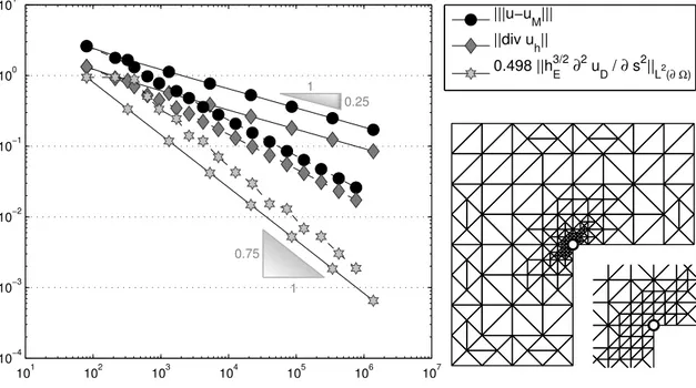
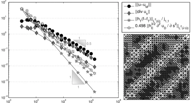
hot`c1ηď∥σ´σh∥L2pΩqďc2η`hot. (1.2) Adaptive refinement based on local contributions toηleads to improved convergence rates of the energy error and so to more economic use of CPU time and the memory that is needed to represent a solution with a certain quality. Figure 1.2 compares the energy error~u´uh~ – ∥σ´σh∥L2pΩqbetween the exact flux and the discrete flux of the P1 conforming finite element method for some Poisson model problem on an L- shaped domain. The adaptive mesh refinement automatically detects singularities like the reentrant corner in this example and leads to optimal convergence rates. However, the proper choice of refinement indicators, at least for the Poisson model problem, is well-understood, so this is only a side aspect of this thesis.
Guaranteed Upper Error Bounds
The main focus in this thesis lies on guaranteed upper bounds (called “error majorants”
by Repin (1999)), i.e.,c2“1 and computable terms of higher order in (1.2). In all model problems under consideration, the error analysis leads to residuals of the form
Respvq– ˆ
Ω f vdx` ˆ
Ωσh¨∇vdx forvPV– H01pΩq (1.3) and associated dual norms
~Res~Z‹ –sup
vPZRespvq{ ~v~
100 101 102 103 104 105 106 10−3
10−2 10−1 100
0.33 1
0.5 1
|||u−u
h|||
Figure 1.2:Convergence history for the energy error~u´uh~for theP1-conforming finite element solutionuhof the Poisson model problem (1.1) withf ”1 on uniform (solid line) and adaptive (dashed line) meshes as a function of the number of degrees of freedom. The right image shows the adaptive mesh on level 4.
with respect to some test function spaceZĎH1and an energy norm~¨~. For instance, the Poisson model problem (1.1) and its discreteP1conforming finite element solution uh with discrete flux σh – ∇uh lead to Z “ V, ~¨~ – ∥∇¨∥L2pΩq and∥σ´σh∥L2pΩq “
~u´uh~ “ ~Res~V‹. In other applications or for inhomogeneous Dirichlet data further overhead terms appear. Although they are of higher order for smooth data, this thesis includes a thorough analysis and derives explicit constants for these additional terms to allow for guaranteed error control also on arbitrary coarse meshes and for nonsmooth data.
Equilibration Error Estimators
The most efficient guaranteed upper bounds of~Res~‹involve the design of some equi- librated quantityqthat has anL2-measurable divergence divqPL2pΩq, i.e.qPHpdiv,Ωq.
The terminus “equilibrated” means that f `divqis small and spawns overhead terms of higher order that are computable oscillations of f and vanish if f is constant. For the Poisson model problem, this leads to
~Res~V‹ “ ~divpσh´qq~V‹`hotď∥σh´q∥L2pΩq`hot. (1.4) Some popular designs forqwere suggested by Ainsworth and Oden (2000), Braess (2007) or Luce and Wohlmuth (2004) and also the design in Carstensen and Funken (1999) can be identified as an equilibration error estimator. Minimisation of the right-hand side of (1.4) over some discrete subspace of Hpdiv,Ωqleads to mixed or least-square FEMs or the dual error majorants of Repin (1999). Equilibration error estimates are usually quite
sharp, however the estimate in (1.4) is suboptimal, since
~divpσh´qq~‹“sup
ϕPV
ˆ
Ωpσh´qq ¨∇ϕdx“ min
vPH1pΩq∥σh´q´Curlv∥L2pΩq. (1.5) In fact, this is the nature of the Helmholtz decomposition and coincides with the majorant theory of Repin (1999), since everyqp–q´Curlvis again an equilibrated quantity in (1.4) and an error majorant in the sense of Repin. However, the algorithmic exploitation of this identity is not so clear and the computation of the exactq“σor Curlvis as expensive as the solve of the original problem. This thesis suggests to compute an equilibrated quantityqafter Braess or Luce-Wohlmuth first. Then a novel postprocessing computes and subtracts some discrete Curlvand so leads to increased efficiency at low costs.
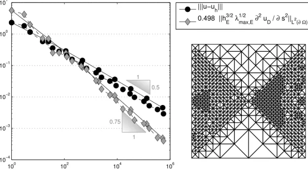
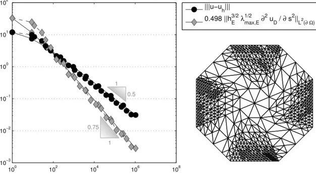
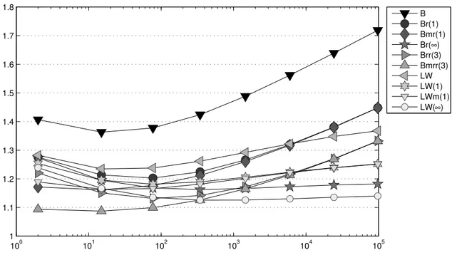
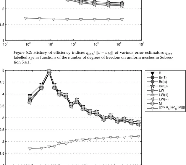
Figure 1.3 displays efficiency indices ∥σh´q´Curlv∥L2pΩq{∥σ´σh∥L2pΩq for some equilibration error estimators after Braess (B) or Luce-Wohlmuth (LW) and the post- processed quantities (Br(1), Brr(3), LW(1)). In this example, the efficiency indices are improved by a factor ten, namely from 1.3 to 1.03 in case of the Braess error estim- ator. Hence, Brr(3) is an almost exact guaranteed upper error bound. More numerical benchmark problems are studied in Chapter 4 also with mixed boundary conditions and discontinuous diffusion coefficients. Moreover, domains with curved boundaries, which cannot be approximated exactly with triangulations into triangles, are considered.
Nonconsistency Residual for Nonconforming Approximations
While the conforming solutions uh are inH01pΩq, the nonconforming approximations uCR by Crouzeix-Raviart finite element methods are not. So the latter ones only allow for a piecewise gradient∇NCuCR, which has also a Curl contribution in its Helmholtz decomposition. In the error analysis for the 2D Poisson model problem (1.1), this leads to a second nonconsistency residual of the form
ResNCpvq–´ ˆ
Ω∇NCuCR¨Curlvdx“ ˆ
ΩCurlNCuCR¨∇vdx forvPH1pΩq.
This residual has the form of (1.3) with f ”0 andσh “CurluCR(and hence permits the application of equilibration error estimators), but there is also the characterisation
~ResNC~H1pΩq‹ “ min
vPH01pΩq∥∇NCpuCR´vq∥L2pΩq.
This implies that any (discrete) conforming approximation v P H01pΩq ofuCR leads to a guaranteed upper bound of~ResNC~H1pΩq‹. Section 4.4 explains several possibilities, also for mixed boundary conditions. One of the most efficient designs in 2D employs the red-refinement and solves local one-dimensional problems to define some piecewise linearvwith respect to the red-refined triangulation.
100 101 102 103 104 105 106 1
1.05 1.1 1.15 1.2 1.25 1.3 1.35
1.4 B
Br(1) Br(∞) Brr(3) LW LW(1) LW(∞) M LS
Figure 1.3:History of efficiency indicesηxyz{ ~e~of various error estimatorsηxyzlabelled xyzas functions of the number of degrees of freedom on adaptive meshes for the Poisson model problem (1.1) with f”1.
Stokes Problem
For given data f : ΩÑR2, the 2D Stokes problem seeks a velocity fielduPH1pΩ;R2q and a pressurepPL2pΩq, such that
´divp∇uq ´∇p“ f and div u“0 inΩ while u“0 onΓD. (1.6) This problem describes the motion of Newtonian fluids, like water. The constraint divu
“0 in (1.6) implies the incompressibility of the fluid, while f is a force that accelerates or decelerates the flow. Since only the gradient of penters, it is unique up to some constant which is commonly fixed with the condition´
Ωpdx“0. The stress tensorσ“∇u`pI solves the Poisson problem´divσ“ f and the error analysis involves a residual of the type (1.3), but, due to the side constraint, is tested with divergence-free functionsZ. In the design of guaranteed upper bounds, this property allows to restrict the investigation to the deviatoric part, i.e.,
~divpσh´qq~Z‹ “ min
vPH1pΩq∥devpσh´q´Curlvq∥L2pΩq.
The divergence constraint also leads to some difficulties in the discretisation. For existence and uniqueness of solutions, the discretisation spaces ofuh P Xhand ph PYh have to satisfy an inf-sup-condition, which reads
0ăc0– inf
qhPYhzt0u sup
vhPXh
´
Ωqhdivpvhq
∥Dvh∥L2pΩq∥qh∥L2pΩq. (1.7)
−1 −0.5 0 0.5 1
−1
−0.8
−0.6
−0.4
−0.2 0 0.2 0.4 0.6 0.8 1
−1 −0.95 −0.9 −0.85 −0.8
−1
−0.98
−0.96
−0.94
−0.92
−0.9
−0.88
−0.86
−0.84
−0.82
−0.8
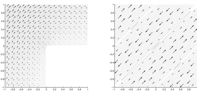
Figure 1.4:Streamlines of Stokes Example with driven cavity on a square domain and zoom-in for the Moffatt eddies in the lower left corner.
It turns out thatP1conforming elements forXhandP0orP1conforming elements for Yhyieldc0 “0, and hence lead to an unstable discretisation scheme. The simplest stable finite element method is the mini finite element method that enriches the velocity space with cubic element bubble functions. Another popular finite element for this application is the Taylor-Hood finite element that pairsP2elements (or the isomorphicP1elements on the red-refinement) for the velocity withP1elements for the pressure.
The nonconforming discretisation, however, is stable also for the lowest-order Crou- zeix-Raviart finite elements. Moreover, the selection of divergence-free Crouzeix-Raviart functions also allows the elimination of the pressure and the divu “0 constraint. Fig- ure 1.4 shows the velocity field and streamlines for some simulation of a lid-driven cavity flow with f ”0 and inhomogeneous Dirichlet data. The zoom of the lower right corner reveals the characteristic Moffatt eddies.
Variational Inequalities
Variational inequalities involve an energy functional that is to be minimised amongst a certain (convex) set of admissible functions. The obstacle problem in Chapter 6 is the prototype of such a variational inequality and minimises the energy
Epvq– 1 2
ˆ
Ω|∇v|2 dx´ ˆ
Ω f vdx (1.8)
amongst the set of functions K–!vPH01pΩqˇ
ˇχďv)
for some obstacle functionχ.
Figure 1.5:Energy minimiseruh without an obstacle constraint (left) and for some (gray- shaded) cusp-shaped obstacleχďuh(right) and f” ´2.
The weak formulation characterises the exact solutionuPKby the variational inequality ˆ
Ω∇u¨∇pu´vqdxď ˆ
Ω fpu´vqdx for allvPK.
Details can be found in the literature, e.g. in Kinderlehrer and Stampacchia (1980). Fig- ure 1.5 displays two solutions for the energy minimisation problem with f ” ´2. The right picture shows the minimiser for some cusp-shaped obstacle and the left picture shows the minimiser without an obstacle constraint which is in fact the solution of the Poisson problem with right-hand side f.
While the unconstrained solutionsuanduh satisfy~Res~‹ “ ~u´uh~, this identity does not hold for the constrained solutions of the obstacle problem. The residual of (1.3) does not take into account the contact force in the part of the domain whereuhtouches the obstacleχ. The revelating view of Braess (2005) on the obstacle problem identifies the discrete solutionuhas the solution of an auxiliary Poisson problem for the right-hand side f´Λhwith some nonunique discrete contact forceΛh. Then, the energy error equals
~u´uh~ ď ~Resaux~‹`overhead terms,
where Resaux is the residual for the auxiliary Poisson problem. The discrete contact forceΛh, however, has to satisfy certain properties, and there are few suggestions in the literature how to realise them. The choice of Carstensen and Merdon (2012) is improved in this thesis in some aspects, e.g., rigorous analysis and explicit constants for all overhead terms and the considerations of extra errors due to inexact solve. This allows guaranteed error control also for inexact discrete solutions (an exact solve is in general infeasible here) that violate the discrete complementary conditions. Efficiency is proven for affine obstaclesχ.
Structure of this Thesis
This thesis is structured as follows. Chapter 2 explains all theoretical preliminaries such as Sobolev spaces, finite element spaces, triangulations and the three finite element methods
of Figure 1.1 for the Poisson model problem. It also gives a brief introduction to the data structures and theMATLABimplementation.
Chapter 3 motivates and studies residuals of the form (1.3). The chapter continues with an explanation of the equilibration error estimator design after Braess and Luce- Wohlmuth and of the Curl postprocessing. The final part of the chapter concerns the standard residual-based error estimator and its efficiency as well as a novel variant with explicit reliability constants that render it a guaranteed upper bound.
Chapter 4 studies a generalised Poisson model problem with mixed homogeneous boundary conditions and a discontinues diffusion tensor, also for three dimensions and domains with curved boundaries. For all three finite element methods under considera- tions, guaranteed upper bounds for the energy error are derived and validated in many numerical benchmark examples from the literature.
Chapter 5 concerns the Stokes problem and commences with the discretisation by the mini finite element method and its error analysis, which is valid also for other con- forming discretisations. The second part studies the nonconforming discretisation with Crouzeix-Raviart elements. The efficiency of the derived guaranteed upper bounds for both methods is examined in five benchmark problems.
Chapter 6 studies the obstacle problem. The first part introduces the setting of this variational inequality and its conforming discretisation. Then, the details of the Braess methodology are explained to achieve guaranteed upper bounds for the energy error with several overhead terms and explicit constants. Moreover, efficiency for affine obstacles is proven and verified in some numerical benchmark examples.
Appendix A shows the main parts of theMATLABimplementation and gives an over- view of the content of the data carrier that comes with this thesis.
Appendix B lists and explains all notation that is used throughout the thesis.
Conclusions and Outlook
The main conclusion of this thesis is that guaranteed error control with sharp efficiency indices is indeed possible for all problems under considerations with a typical overestim- ation of the guaranteed error bound by a factor 1 to 4.
The suggested postprocessing allows improvement of the efficiency of any equilibration error estimator at very low extra effort. Naturally, the gain of efficiency is limited by the influence of the overhead terms. They are the reason for the slightly worse efficiency indices in the numerical examples for the Stokes problem (about 1 to 4) compared to the efficiency indices for Poisson problems (close to 1). The rather pessimistic values for the constantc0from (1.7), which enter the guaranteed upper bounds, lead to some unnecessary overestimation. Better knowledge and improved guaranteed lower bounds for c0, e.g., by numerical solve of the associated general eigenvalue problem, might improve the efficiency of the error estimators dramatically. For obstacle problems, at least those with affine obstacles, the overhead terms are of higher order and yield efficiency indices between 1 and 2. The combination of the postprocessing with the mean correction is able to reduce the influence of the oscillation terms on coarse meshes.
However, the theory of this thesis is not limited to these three problems and also not limited to error control in terms of energy norms. Further applications include linear elasticity, convection-diffusion-reaction partial differential equations or nonlinear
problems as Poisson problems with friction. All techniques also transfer to parabolic partial differential equations. Furthermore, goal-oriented error estimation is possible through duality techniques and Riesz representation of the goal functional. The efficiency of the error estimators for the energy norm directly influences the sharpness of the guaranteed bounds for the goal error.
A further challenge, vital to nonlinear problems, is the inexact solve. In this case the discrete solution looses its Galerkin orthogonality property which is a prerequisite for the equilibration designs of Braess and Luce-Wohlmuth. However, as in the case of obstacle problems, the discrete solution solves a perturbed problem with a different right-hand side that can be analysed instead and causes another extra term in the guaranteed upper bound that measures the truncation error of the iterative solver.
Acknowledgements
These last lines of the introduction I want to dedicate to all the people that helped me to realise this thesis. That includes foremost my doctoral advisor Prof. Carsten Carstensen who taught me almost everything I know now about finite element methods, error estimation and paper writing. I also want to thank my colleague Wolfgang Boiger who became a valuable friend during our research stays in the Republic of Korea in 2009 and 2010. I learned so much practical things from him, like git and tikz, that helped me to write up this thesis fast and efficiently. Finally, I want to thank all my other colleagues and friends and my family for their support during the last years.
This chapter recalls theoretical preliminaries needed for the mathematical modeling and the numerical analysis in the thesis.
2.1 Functional Analysis for Sobolev Spaces
The following section gives a very short introduction to Sobolev spaces. A complete and more detailed introduction can be found in textbooks like Grisvard (1985) or Evans and Gariepy (1992).
2.1.1 Sobolev Spaces
Here and throughout, Ω Ă Rn denotes some Lipschitz domain inn “ 2 or n “ 3 di- mensions with polygonal or polyhedral boundaryBΩand outer normal vectorν. The boundary may consist of some closed Dirichlet partΓD with positive surface measure and some (possibly empty) Neumann partΓN –BΩzΓD. The spaceLppΩ;Rmqdenotes the Lebesgue spaces ofLp-integrable functions overΩwithmcomponents andLlocp pΩq contains all functions that areLp integrable on every open subsetωĂĂ Ωthat is com- pactly contained inΩ. The function spaceCkCpΩ;Rmqdenotes allktimes differentiable functions with compact support inΩ, whileCDpΩ;Rmqdenotes the continuous functions with zero boundary conditions alongΓD.
Definition 2.1.1(Weak Derivative). The function gj PL1locpΩ;Rmqis called aweak derivative of v PL1locpΩ;Rmqwith respect to xj, j“1, . . . ,n, if the integration by parts formula
ˆ
Ωv¨ Bϕ{Bxjdx“ ´ ˆ
Ωgj¨ϕdx holds for all ϕPCC1pΩ;Rmq.
In this case, gj is abbreviated withBv{Bxjand if all partial derivatives exist,Dv“ pBv{Bx1, . . . , Bv{Bxnq PL1locpΩ;Rmˆnqdenotes the weak gradient of v.
Definition 2.1.2(Sobolev Spaces). TheSobolev spaceH1consists of all L2functions whose weak gradient is also in L2, i.e.,
H1pΩ;Rmq–␣
vPL2pΩ;Rmqˇ
ˇDvPL2pΩ;Rmˆnq( . The space of all L2functions with divergence in L2reads
Hpdiv,Ω;Rmˆnq–␣
vPL2pΩ;Rmˆnqˇ
ˇdivvPL2pΩ;Rmq( .
Definition 2.1.3(Dual Space and Dual Norm). Thedual space B‹ of some Banach space B with respect to the norm ∥¨∥ consists of all bounded linear functionals F : B Ñ R, i.e.
B‹– LpB,Rq, and thedual normof some FPB‹ reads
∥F∥‹– sup
vPBzt0u
Fpvq{∥v∥.
Remark 2.1.4. The dual space of LppΩ;Rmqis (by Hölder inequality) the space LqpΩ;Rmqwith 1{p`1{q“1.
In the following, the codomain of a function space is omitted ifm“1, e.g.,L2pΩ;R1q “ L2pΩqandHpdiv,Ω;R1ˆnq “Hpdiv,Ωq. Moreover,∇v“Dvdenotes the derivative for scalar-valued functionsvPH1pΩq.
2.1.2 Traces of Sobolev Functions
Since Lebesgue function are defined up to sets of measure zero, the existence of well- defined traces inL2pBΩqalong the boundaryBΩis not obvious. However, under certain regularity assumptions they exist.
Theorem 2.1.5(Existence of Traces (Evans and Gariepy, 1992; Temam, 2001)). For a bound- ed Lipschitz domainΩthere exists a bounded linear operator T: H1pΩq Ñ L2pBΩq, calledtrace operator, such that
(a) Tpvq “v onBΩfor all vPH1pΩq XCpΩq, and, (b) for all qPHpdiv,Ωqand vPH1pΩq, it holds
ˆ
BΩTpq¨νqvds“ ˆ
Ωvdivqdx` ˆ
ΩDv¨qdx.
Proof. The proof of (a) studies Tpvqpyq–lim
rÑ0 Bpr,yqXΩvpxqdx foryP BΩandvPH1pΩq
and can be found in Evans and Gariepy (1992, Theorem 1 on page 133). A proof of (b) is given in Temam (2001, Theorem 1.2 on page 7) whereHpdiv,Ωqis named asEpΩq.
Remark 2.1.6. Actually, the normal flux qν in the left-hand side of (b) is an element of the dual space H´1{2pBΩqof H1{2pBΩq Ą L2pBΩq. Therefore, the integral is to be understood in a distributional sense. However, to facilitate a simple notation we abide by the integral notation and usually we consider Hpdiv,Ωqfunctions with trace in L2pBΩq. Moreover, T is omitted in the sequel.
Definition 2.1.7. The space of functions with zero trace alongΓDreads HD1pΩq–tvPH1pΩqˇ
ˇv“0alongΓDu.
2.1.3 Basic Inequalities
This subsection collects some basic inequalities related to Sobolev spaces. Although these inequalities are formulated for scalar-valued functions here, they hold verbatimly for vector-valued functions.
Theorem 2.1.8(Poincaré Inequality). LetΩbe a Lipschitz domain with C1boundary. There exists a constant CPpΩqofΩsuch that, for any function vPH1pΩqwithffl
Ωv“0, it holds
∥v∥L2pΩqďCPpΩqdiampΩq∥∇v∥L2pΩq. The constant CPpΩqis invariant under rescaling ofΩ.
Proof. A proof can be found in Evans (2010, Theorem 1 on page 275).
Remark 2.1.9. On convex domainsΩĂRnin any dimension nPN, it holds CPpΩq ď 1{π (Payne and Weinberger, 1960; Bebendorf, 2003). For triangular domains TĂR2, Laugesen and Siudeja (2010) recently showed the refined result CPpTq ď1{j1,1with the first positive root j1,1of the Bessel function J1.
Theorem 2.1.10 (Friedrichs Inequality). Let Ω be a Lipschitz domain and Γ Ă BΩ with nonzero n´1dimensional Hausdorff measure. There exists a constant CFpΩ,Γqsuch that, for any function vPH1pΩqwith v“0alongΓ, it holds
∥v∥L2pΩqďCFpΩ,ΓqdiampΩq∥∇v∥L2pΩq. The constant CFpΩ,Γqis invariant under rescaling ofΩ.
Proof. A proof can be found in Braess (2007, page 30).
Theorem 2.1.11(Trace Theorem). LetΩbe a Lipschitz domain andΓĂ BΩwith nonzero n´1 dimensional Hausdorff measure. Then there exists a constant CTpΩq, such that, for any function vPH1pΩqwith v“0alongΓ, it holds
∥v∥L2pBΩqďCTpΩ,ΓqdiampΩq1{2∥∇v∥L2pΩq. The constant CTpΩ,Γqis invariant under rescaling ofΩ.
Proof. Brenner and Scott (2008, Theorem 1.6.6 on page 39) prove
∥v∥L2pBΩq ďC∥v∥1{2L2pΩq∥∇v∥1{2L2pΩq.
A Friedrichs inequality estimates∥v∥1{2L2pΩqon the right-hand side and concludes the proof withCTpΩ,Γq–CCFpΩ,Γq1{2.
2.1.4 Helmholtz Decomposition
The following theorem establishes the Helmholtz decomposition of vector fields into some gradient and some Curl defined as
Curlv–
ˆ0 ´1
1 0
˙
∇v“
ˆ´Bv{Bx2 Bv{Bx1
˙
forn“2 andvPH1pΩq,
Curlv–∇ˆv“
¨
˝
Bv3{Bx2´ Bv2{Bx3
Bv1{Bx3´ Bv3{Bx1 Bv2{Bx1´ Bv1{Bx2
˛
‚ forn“3 andvPH1pΩ;R3q.
(2.1)
To handlen“2, 3 simultaneously, assumes– 1 forn“2 ands–3 forn “3. For the following theorem, recall Definition 2.1.7 ofHD1pΩqand recall thatνdenotes the outer unit normal vector ofΩalongBΩ.
Theorem 2.1.12(Helmholtz Decomposition). LetΩbe a bounded (simply connected) Lipschitz domain. Given any pPL2pΩ;Rnqand a symmetric, uniformly positive tensorSPL8pΩ;Rnˆnq, there existαPH1DpΩqandβPH1pΩ;RsqwithCurlβ¨ν“0onΓN such that
Sp“S∇α`Curlβ.
This split is orthogonal in the sense that (a) ´
ΩpSpq ¨∇vdx “´ΩpS∇αq ¨∇vdx for all vPH1DpΩq (b) ´
Ωp¨Curlwdx“´
ΩpS´1Curlβq ¨Curlwdx for all wPH1pΩ;Rsq.
Proof. The Lax-Milgram theory yields a unique solutionαPH1DpΩqfor (a) withS∇α¨ν“ Sp¨νalongΓN. The remainderq–Spp´∇αqis divergence-free, i.e.qPHpdiv,Ωqwith divq“ 0, and satisfiesq¨ν “0 along ΓN. Standard results in higher analysis, such as Theorem 3.1 (for n “ 2) and Theorem 3.4 (forn “ 3) from Girault and Raviart (1986) ensure the existence of someβPH1pΩ;Rsqwithq“Curlβ. An integration by parts and a density argument yields (b).
2.2 Finite Element Spaces
Weak formulations of the model problems in this work lead to the test function spaces H01pΩqand Hpdiv,Ωqas well asL2pΩq. Finite element methods discretise these spaces and employ generalised splines on subdomains, i.e. triangles or tetrahedra. This section introduces suitable ansatz functions for a single subdomain, while the next section in- troduces regular triangulations which connect these subdomains and allow for global interpolation on the whole domain.
2.2.1 Finite Elements in the Sense of Ciarlet
The following introduction to finite elements follows the outline in Brenner and Scott (2008) and the basic concepts of Ciarlet (1978).
Definition 2.2.1(Finite Element in the Sense of Ciarlet (1978)). The triplepT,P,Lqdefines a finite element in the sense of Ciarlet if
Figure 2.1:Lagrange (1-3), Crouzeix-Raviart (4) and Raviart-Thomas finite elements (5).
1. TĂRnis a bounded closed set with nonempty interior and piecewise smooth boundary, 2. Pis a finite-dimensional space of functions on T,
3. L“ tL1,L2,¨ ¨ ¨,LNuis a basis ofP‹.
2.2.2 Lagrange, Crouzeix-Raviart and Raviart-Thomas Finite Elements
This subsection introduces the three best-known finite element classes illustrated in Figure 2.1. The markings in this figure relate to the linear functionals L1,L2, . . . ,LNor the degrees of freedom of the finite elements. In the following,δjk refers to the Kronecker delta, i.e.,δjk“1 if j“kandδjk“0 otherwise.
Definition 2.2.2(Local Polynomial Spaces). Given some triangle (for n“2) or tetrahedron (for n “ 3) T, the polynomials of degree k are denoted byPkpTq. The set of Raviart-Thomas functionsof order k on T reads
RTkpTq–␣
vPPk`1pT;Rnqˇ
ˇDa0,a1, . . . ,anPPkpTq @xPT,vpxq “ pa1, . . . ,anq `a0x( . Definition 2.2.3(Local Nodal Basis Function). Given some triangle (for n“2) or tetrahedron (for n “3) T“convtP1, . . . ,Pn`1u, thelocal nodal basis functionϕPj of the node Pjis defined by
ϕPj PP1pTq and ϕPjpPkq “δjk for all k“1, . . . ,n`1.
Remark 2.2.4. The nodal basis functionsϕP1, . . . ,ϕPn`1 coincide with the barycentric coordinates in the sense that, for every x PT, it holds
x“
n`1ÿ
j“1
ϕPjpxqPj and n`1ÿ
j“1
ϕPj ”1.
Furthermore, they define a basis ofP1pTq.
Theorem 2.2.5(Lagrange Finite Elements). Let T “ convtP1, . . . ,Pn`1ube some triangle (for n “2) or tetrahedron (for n “3) with centermidpTqand sides E1, . . . ,En`1enumerated as shown in Figure 2.2, i.e. Ej – convtPkˇ
ˇk “ 1, . . . ,n`1 &k ‰ ju. The points Rjk :“
pPj`Pkq{2denote the edge midpoints for1 ďjă kď n`1(and coincide with the centers of E1, . . . ,E3for n“2). Furthermore, consider the point evaluationsϱxpvq–vpxqfor vPP2pTq and any xPT.
(a) The triplepT,P0pTq,pϱmidpTqqqdefines a finite element in the sense of Ciarlet.
P1
P2 P3
E3
E1 E2
Figure 2.2:Standard enumeration of vertices and faces in a triangle. The vertexPjis opposite to the faceEj.
(b) The triplepT,P1pTq,pϱP1, . . . ,ϱPn`1qqdefines a finite element in the sense of Ciarlet.
(c) The triplepT,P2pTq,pϱP1, . . . ,ϱPn`1,ϱRjk for1ďjăkďn`1qqdefines a finite element in the sense of Ciarlet.
Proof. Assertion (a) is trivial. The barycentric coordinatesϕP1, . . . ,ϕPn`1 define a basis of P1pTq. SinceϱPjpϕPkq “δjk and dimP1 “dimP1‹ “ n`1, the functionalsϱP1, . . . ,ϱPn`1 define a basis ofP1pTq‹. This proves (b). For (c) andP2pTqwith dimension dimP2pTq “ pn`2qpn`1q{2, consider the same number of functions
ϕˆPj “ϕjp2ϕj´1q forj“1, . . . ,n`1 and ˆ
ϕRjk “4ϕPjϕPk for 1ďjăkďn`1.
These functions satisfyϱXpϕˆYq “δXYfor anyX,YP tP1,P2,P3,Rjkfor 1ďjăkďn`1u and therefore are a valid dual basis.
Theorem 2.2.6 (Crouzeix-Raviart Finite Element). Let T “ convtP1, . . . ,Pn`1u be some triangle (for n“2) or tetrahedron (for n“3) with sides E1, . . . ,En`1as in Theorem 2.2.5 with associated linear functionals
Ljpvq–
Ej
vds for j“1, . . . ,n`1and vPP1pTq The Crouzeix-Raviart basis functions
ψjpxq–1´nϕj for j“1, . . . ,n`1
form a dual basis forpL1, . . . ,Ln`1qand so the triplepT,P1pTq,pL1, . . . ,Ln`1qqdefines a finite element in the sense of Ciarlet.
Proof. By linearity, it follows ϕjpmidpEkqq “ p1´δjkq{nand the Crouzeix-Raviart basis functions satisfyψjpmidpEkqq “δjkand so form a dual basis oftL1, . . . ,Ln`1u.
Theorem 2.2.7 (Raviart-Thomas Finite Element). Let T “ convtP1, . . . ,Pn`1u be some triangle (for n“2) or tetrahedron (for n“3) with sides E1, . . . ,En`1as in Theorem 2.2.5 with associated linear functionals
Ljpvq– ˆ
Ej
v¨νT|Ejds for j“1, . . . ,n`1and vPRT0pTq
whereνTdenotes the outer unit normal vector of T alongBT. These functionals and the Raviart- Thomas basis functions
ϑjpxq– 1 n|T|
`x´Pj˘
for j“1, . . . ,n`1.
satisfy
(a) Ljpϑkq “δjk,andϑkpxq ¨νT|Ej “δjk{
Ej
for xPEj, (b) the settϑ1, . . . ,ϑn`1uis a basis ofRT0pTq, and
(c) the triplepT, RT0pTq,pL1,L2, . . . ,Ln`1qqdefines a finite element in the sense of Ciarlet.
Proof. Easy geometrical considerations showpx´Pjq ¨νT|Ej “n|T|{Ej
forx PEj and px´Pkq ¨νT|Ej “0 forxPEjandk ‰j. This proves (a). For the proof of (b) it is easy to check thatϑj PRT0pTqforj“1, . . . ,n`1 and their linear independency follows from (a).
Since, dimpRT0pTqq “n`1 this proves (b). The last assertion (c) follows directly from (a) and (b) similar to the theorems above.
2.2.3 Regular Triangulations and Related Notation
Triangulations are the main tool for domain discretisation in finite element methods and are the topic of this subsection.
Definition 2.2.8(Triangulation). AtriangulationT of some polyhedral Lipschitz domainΩ consists of n-dimensional closed triangles (for n “2) or tetrahedra (for n “3) T P T, called elements, such thatŤ
TPT “ Ω. The set of all vertices in the triangulation is denoted by N and the set of all sides (edges for n “2and faces for n “3) in the triangulation is denoted by E. The subsets EpBΩq – tE P EˇˇE Ď BΩucontains all sides along the boundaryBΩ, while EpΩq–EzEpBΩqcontains all interior sides.
Definition 2.2.9(Regular Triangulation). A triangulation is called regular if the intersection of any two elements T1,T2 PT with T1 ‰T2equals T1XT2“∅or
T1XT2 “convtz1, . . . ,zku for1ďkďn nodes z1, . . . ,zk PN.
(Hence, the intersection equals a single node, an edge or a face of the triangulation.) For mixed boundary conditions there is the additional condition that the intersection of any boundary edge EPEpBΩqwithΓD satisfies
EXΓD “E or EXΓD“∅.
Figure 2.3 displays some examples for triangulations that satisfy or violate these condi- tions.
To simplify the presentation in the rest of this thesis some notation is in order. First, there are several local subsets ofE,T andN, namely
NpEq–tzPNˇˇzPEu and TpEq–tT PT ˇˇEĂ BTu forEPE, NpTq–tzPNˇˇzPTu and EpTq–tEPEˇˇEĂ BTu forTPT,
Epzq–tEPEˇˇzPEu and Tpzq–tT PT ˇˇzPTu forzPN.
Figure 2.3:One regular (left) and two non-regular (middle and right) triangulations.
Second, there are different types of patches that are the node patch ωz –int´ď
Tpzq¯ forzPN, the side patch ωE –int´ď
TpEq¯ forEPE, the element patch ωT – ď
zPNpTq
ωz forTPT.
Third, the boundary sidesEpBΩqsplit into the Dirichlet and Neumann sides EpΓDq–tEPEpBΩqˇˇEĎΓDu and EpΓNq– EpBΩqzEpΓDq.
The associated sets of triangles read
TpΓDq–tTPT ˇˇEpTq XEpΓDq ‰∅u and TpΓNq–tTPT ˇˇEpTq XEpΓNq ‰∅u.
Similarly, there there are Dirichlet boundary nodes NpΓDq–tzPNˇˇzPΓDu.
The remaining nodes form the set of free nodes, M–NzNpΓDq.
2.2.4 Interpolation Operators and Finite Element Spaces
This subsection applies the results on finite elements of Subsection 2.2.2 to each element of a regular triangulation and so defines interpolation operators on Ω. Furthermore this subsection defines finite element approximation spaces as the codomains of these operators. Such approximation spaces are required for the finite element methods of Section 2.3.
Definition 2.2.10(Local Interpolant). Let pT,P,Lq be some finite element with dual basis tξ1, . . . ,ξNuof L, i.e., Ljpξkq “ δjk. Furthermore, let v be some function for that Lpvqis well- defined. Then, thelocal interpolationof v on T reads
Ipvq|T – ÿN
j“1
Ljpvqξj.
TheT-piecewise application of the local interpolant to a function inC8pΩqleads to an interpolant that is defined onΩ. This global interpolant is broken in the sense that it is possibly discontinuous along sides of the triangulation. However, depending on the structure of the finite element, there are some continuity properties. The following definitions introduce broken polynomial spaces and global basis functions to formalise this.
Definition 2.2.11 (Broken Polynomial Spaces). For a collection T of elements, theset of piecewise polynomialsonŤ
T –ŤTPT T reads
PkpTq–!vPL2´ďT¯ˇˇ@TPT, v|T PP1pTq). Thebroken Raviart-Thomasspace of lowest order k“0reads
RT´1pTq–!vPL2´ďT;Rn¯ˇˇ@TPT, v|T PRT0pTq) .
Definition 2.2.12(Global Basis Functions). For a given regular triangulationT, thenodal basis functionϕz for some node zPN is given by
ϕz PP1pTq, and ϕzpyq–
#1 for z“y, 0 for z‰yPN.
Similarly, theCrouzeix-Raviart basis functionψEfor some side EPE is given by ψE PP1pTq, and ψEpmidpFqq–
#1 for E“F, 0 for E‰FPE.
Locally, these global basis functions coincide with the local basis functions of Theorems 2.2.5 and 2.2.6.
Finally, theRaviart-Thomas basis functionϑE PRT´1pTqfor some side EPE with some arbitrary but fixed oriented normal vectorνEis given by
ϑEpxq|T –pνE¨νTq 1
n|T|px´Pq in xPT“convtE,Pu PTpEq.
Furthermore ϑ ” 0 on T P TzTpEq. Locally, the function ϑE coincides with the local basis functions of Theorem 2.2.7 on T PTpEqup to the signνT¨νE P t´1, 1u.
Remark 2.2.13. Subsubsection 2.3.5.5 below explains how the orientation is fixed in the imple- mentation for this thesis.
Notice thatϕzis continuous inΩand thatψE is continuous in the midpoint midpEqof the sideEPE. The functionϑE¨νEis continuous along the sideEPE. These continuity properties are reflected in the following definitions of the interpolation operators and their codomains.
Definition 2.2.14(Nodal Interpolation andP1Conforming Finite Element Space). The application of the local interpolant of theP1Lagrange finite element with the nodal basis functions