LIMNOLOGY and OCEANOGRAPHY: METHODS

A toolbox for secondary quality control on ocean chemistry and hydrographic data

Siv K. Lauvset,*

Toste Tanhua

1Geophysical Institute, University of Bergen and Bjerknes Centre for Climate Research, Bergen, Norway

2Helmholtz Centre for Ocean Research Kiel (GEOMAR) – Marine Biogeochemistry, Kiel, Germany

Abstract

High quality, reference measurements of chemical and physical properties of seawater are of great impor- tance for a wide research community, including the need to validate models and attempts to quantify spatial and temporal variability. Whereas data precision has been improved by technological advances, the data accuracy has improved mainly by the use of certified reference materials (CRMs). However, since CRMs are not available for all variables, and use of CRMs does not guarantee bias-free data, we here present a recently developed Matlab toolbox for performing so-called secondary quality control on oceanographic data by the use of crossover analysis. This method and how it has been implemented in this toolbox is described in detail. This toolbox is developed mainly for use by sea-going scientists as a tool for quickly assessing possible bias in the measurements that can—hopefully—be remedied during the expedition, but also for possible post-cruise adjustment of data to be consistent with previous measurements in the region. The toolbox, and reference data, can be downloaded from the Carbon Dioxide Information Analysis Center (CDIAC): http://

cdiac.ornl.gov/ftp/oceans/2nd_QC_Tool_V2/.

Chemical and physical hydrographic measurements in the ocean have a long history during which the quality of the measurements have, in general, increased with time. With the quality of a measurement we mean both the precision and the accuracy; the latter being of great importance for inter-comparability of measurements conducted by different research teams, and for the quantification of temporal and spatial variability or trends. The accuracy of measurements can be increased by the use of certified reference materials (CRMs) as is common practice for carbonate system measure- ments and salinity. For instance, the introduction of CRMs for dissolved inorganic carbon (DIC) and total alkalinity dur- ing the WOCE period practically eliminated cruise-to-cruise biases in these parameters (e.g., Johnson et al. 1998). How- ever, CRMs are not available for all variables or used on each cruise and measurements performed without the aid of CRMs are more prone to show biases, although the use of CRMs is no guarantee for accurate measurements as several factors

can lead to biases, such as incorrectly quantified standard concentrations, the CRM concentration range being different from the samples, or other analytical difficulties. Overall, improvements in the instrumentation has reduced the achievable precision to about 2lmol kg²¹for DIC and, with the use of CRMs, an accuracy better than 5lmol kg²¹can be routinely obtained. We strongly recommend using CRMs whenever possible for your measurements, to increase the accuracy of oceanographic data, and for facilitating detection and quantification of trends.

One way of verifying the accuracy of measurements con- ducted during an oceanographic cruise is by so-called second- ary quality control (2^ndQC). It is important to note that 2^nd QC only addresses the accuracy of the data, not the preci- sion, of the measurements. The precision of the measure- ments is naturally very important, but while it is accounted for during 2^nd QC it is more appropriately evaluated in pri- mary quality control routines. The most important tool in the 2^nd QC process is the crossover analysis, although not the only one available. This is an objective comparison of deep water data from one cruise with data from other cruises in the same area (Sabine et al. 1999; Gouretski and Jancke 2001; Johnson et al. 2001; Tanhua et al. 2010) based on the assumption that the deep ocean (typically>1500 m) is invariant. Differences in the reported values obtained during different ship campaigns can be due to systematic biases in, Additional Supporting Information may be found in the online version of

this article.

*Correspondence: siv.lauvset@uib.no

This is an open access article under the terms of the Creative Commons Attribution License, which permits use, distribution and reproduction in any medium, provided the original work is properly cited.

and

OCEANOGRAPHY: METHODS

at least, one of the measurements. Obviously, care has to be exercised so that real trends and variability are not wrongly interpreted as biases. This is particularly critical for areas of the deep ocean that are rapidly ventilated or close to fronts and major currents. We do recommend that the use of cross- over analysis is considered already at the cruise planning state, so that stations are deliberately planned to colocate with historic cruises, which is routinely applied to the plan- ning of programs like GEOTRACES and GO-SHIP. This is not only beneficial for 2^nd QC purposes, but can also be useful for detecting trends in ocean variables.

Crossover analyses were performed on a large scale for the WOCE data during the construction of the Global Ocean Data Analysis Project (GLODAP) (Key et al. 2004) data collec- tion (e.g., Gouretski and Jancke 2001; Johnson et al. 2001;

Sabine et al. 2005), and was further developed during the Carbon in Atlantic Ocean (CARINA) project (Tanhua et al.

2010). Similar routines as those developed during CARINA were later used for Pacific Ocean Interior Carbon (PACIF- ICA), and for the new version of GLODAP (i.e., GLODAPv2), see below. Typically for these projects, all offsets between all available crossovers for an ocean basin are calculated, and these offsets are then compared to each other by the use of least square models (e.g., Wunsch 1996), typically using the inversion scheme described by Johnson et al. (2001). The inversion then seeks a solution that minimizes the bias between cruises, i.e., the inversion makes suggestions on how individual cruises should be adjusted to produce the most internally consistent data collection possible. During this step, it is possible to assign weights to the crossover results that go into the inversion based on, for instance, the time-lag between the occupations of a station-pair (i.e., a crossover weighs more heavily if the repeat of a station was performed within a short time-frame), the uncertainty of the crossover, and crossovers in an ocean region with small vari- ability far away from ocean fronts could weigh more heavily.

We will here describe a Matlab toolbox that performs 2^nd QC on deep ocean carbon chemistry and hydrographic data by comparing new data files to the quality-controlled data product GLODAPv2. The principles of the toolbox can be used to create a modified version that can to be used with different reference data set including other variables. This can be useful for, for instance, variables measured during various legs of GEOTRACES. This 2^ndQC toolbox is intended to be a dynamic tool; to be changed and improved over time as scientists begin to use it and to develop new uses for it.

Currently, since this is the background and expertise of the authors, it is made to easily assess chemical and hydrograph- ical oceanographic data. However, modifying the 2^nd QC toolbox to assess other oceanographic data is possible, and every user should feel free to do this.

It is important to note the difference between the 2^ndQC process carried out by this toolbox, and the 2^ndQC that was

applied to data products like GLODAPv2, PACIFICA or CARINA. The main difference is in the step following the crossover analysis: in the making of the above data products, the results of the crossovers were fed into an inversion in which all cruises could be adjusted using a least square model, whereas in this toolbox the reference cruises are not adjustable so that the inversion step is not needed. The ana- lyst is, in essence, comparing the result with a reference data set that is not changing. This assumes that the reference dataset is not biased, an assumption that might not be per- fectly valid as new data, particularly to less sampled areas of the ocean, can eventually lead to adjustments of the refer- ence dataset (although that is slightly outside of the scope of this article). However, as the GLODAPv2 data product is planned updated with new cruises regularly the reference data used with this toolbox can safely be assumed unbiased.

The 2^nd QC toolbox presented here consists of several scripts and functions (Supporting Information Appendix A), most of which are modified versions of the scripts and func- tions used by the CARINA project (Tanhua et al. 2010, avail- able for downoad: cdiac.ornl.gov/oceans/2nd_QC_Tool/). In the following sections, we will discuss the underlying princi- ples of crossover analysis and describe the 2^ndQC toolbox in some detail.

Methods and tools

The crossover analysis

A crossover analysis objectively analyses the differences between two cruises conducted in the same area by compar- ing measurements in the deep part of the water column (typically>1500 m). The result of a crossover analysis is the mean weighted difference between several stations on two different cruises, which is referred to as the offset. If data precision in at least one of the cruises is poor, or the area is highly variable, this offset will have a large standard devia- tion. Offsets can be defined either as additive or multiplica- tive difference between two cruises, A (the cruise being analyzed) and B (a cruise from the reference data set). If the offset is zero (or unity for multiplicative parameters) then cruises A and B are unbiased for that parameter.

Initially the crossover routine seeks stations from the ref- erence data set which have measurements of the parameter in question, and are within a predefined radius of the sta- tions being analyzed. This radius is commonly set to 200 km (28 arcdistance), but can be freely defined by the analyst based on the expected spatial variability in the region and the availability of reference data. The next step in the crossover analysis is to interpolate each data profile with a piecewise cubic hermite interpolating scheme (Fritsch and Carlson 1980). Note that this interpolation is always performed in depth space. An important feature of this scheme is that interpolated values almost never exceed the range spanned by the data points and that large vertical gaps

in the data are not interpolated. The definition of “large” is depth-dependent so that larger gaps are allowed in the deeper part of the profile (Table 1).

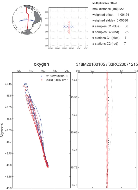
The interpolated profiles from cruise A and B are compared with the “running-cluster” routine (Tanhua et al. 2010) in which each station from cruise A is compared to all stations from cruise B within the maximum distance for a valid cross- over. This is repeated for all stations from cruise A and the average difference profile and the weighted standard deviation can be calculated and graphically displayed for each cruise- pair; see Fig. 1 for an example. By using a weighted mean off- set, the parts of the profiles with low variability (or high preci- sion) have more weight in the calculation of an offset. The offset is thus always the bias in cruise A with respect to cruise B, where we assume that cruise B—the reference cruise—repre- sents the correct value. This process is repeated for all cruises in the reference data product. An overview plot is then created showing the weighted mean offset and its standard deviation for all crossovers found for cruise A vs. the reference data; see Fig. 2 for an example. The offset toward the reference cruises are plotted vs. the year of the reference cruises so that tempo- ral trends for the area can be identified and considered in the suggestion of an adjustment (Fig. 2). Offsets for cruise A less than zero (or unity for multiplicative parameters) suggests that cruise A data would have to be increased to be consistent with cruise B—i.e., it would get a positive adjustment (or a greater than one multiplicative adjustment)—and vice-verse.

Based on all the offsets calculated for a cruise, the investigator can make a decision on whether or not there is a bias in the measurements.

At this stage it is important to pay attention to the

“goodness” of the crossovers. This is primarily indicated by the weighted standard deviation of the offset, but factors such as the proximity to active frontal regions or regions with high variability in the deep water increase the chance that an offset is found for unbiased data. The number of crossover cruises is another important consideration as a bias determined based on comparison with just a few reference cruises is much more uncertain than a bias determined based on several reference cruises spanning several years. In an ideal case a problem in the analytical routines can be identi- fied and eliminated, while in other cases an adjustment can be suggested to make the new data consistent with the refer-

ence data. It cannot be stressed enough that one should never ever adjust the original data based on the offset deter- mined in the 2^nd QC process; a note in the metadata of a possible bias is a better way to convey this result.

Knowledge of normally achievable precision and accuracy of measurements influence to which level an adjustment should be suggested. For the CARINA project, in general no adjustment smaller than 5 ppm for salinity, 1% for oxygen, 2% for makro- nutrients, 4lmol kg²¹for DIC and 6lmol kg²¹for total alka- linity was applied. During GLODAPv2 these levels were slightly modified so that phosphate data were allowed to vary by up to 4% in the Atlantic Ocean and adjustments as small as 4lmol kg²¹ were applied to total alkalinity data, which tend to be very precise, but not quite so accurate (Olsen et al. 2015). For cruises with low data precision (i.e., high uncertainty), it is gen- erally more difficult to do a reasonable 2^ndQC and this will be reflected in high standard deviation of the crossover. The rule of thumb is to always give the data “the benefit of doubt.”

Therefore, if you are not absolutely certain that a cruise has biased data, then do not suggest an adjustment.

Offsets are quantified as multiplicative factors for all the makronutrients (i.e., nitrate, phosphate, and silicate), and oxygen, and as additive constants for salinity, DIC, alkalin- ity, and pH. There are several reasons for the division between additive and multiplicative offsets. First, multiplica- tive offsets eliminate the problem of potentially negative val- ues for any variable with measured concentrations close to zero, i.e., in the surface water for nutrients or in low oxygen areas for oxygen. Also, for nutrients and oxygen analysis problems in standardization are the most likely source of errors, hence a multiplicative offset is deemed the most appropriate. For DIC, alkalinity, and salinity an additive adjustment is more appropriate, since a likely source of error for these parameters is biases in the reference material used (if used). Similarly, since pH is a logarithmic unit only addi- tive offsets can be considered for pH.

Examples of crossover analysis

We here describe three examples of 2^nd quality control that illustrates the use of the method. More detailed infor- mation about these cruises, including crossover plots, can be found at the GLODAPv2 site (http://cdiac.ornl.gov/oceans/

GLODAPv2/cruise_table.html). First, we discuss the offset of alkalinity measurements shown for a cruise on the R/VG.O.

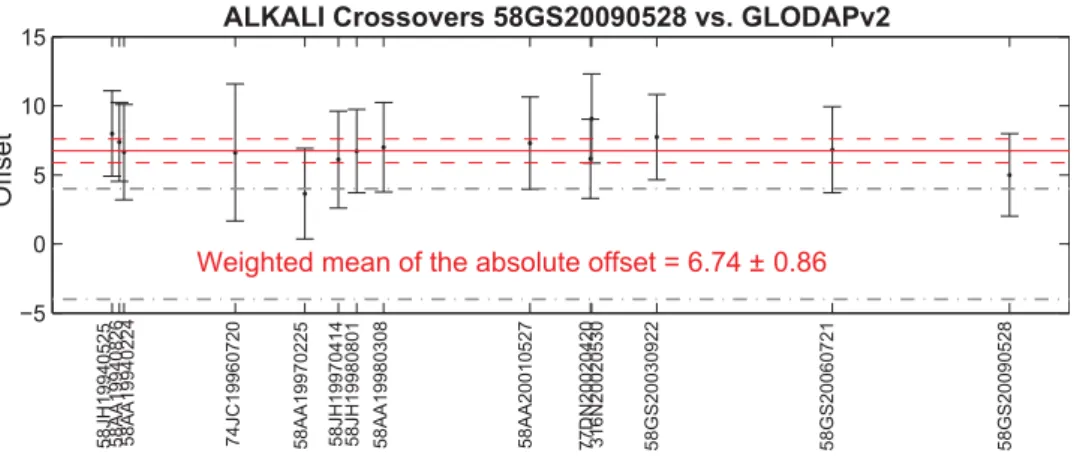
Sars to the Nordic Seas (58GS20090528, Fig. 3). During this cruise the PIs used, and corrected to, CRMs, but a significant and consistent offset is still clearly seen in the data, suggest- ing that the cruise should be adjusted downward. In fact, alkalinity for this cruise is adjusted with 25 lmol kg²¹ for alkalinity in GLODAPv2. This is an example for cases when the use of CRMs did not prevent a bias to be present.

A second example is the silicate data for a cruise to the tropi- cal Atlantic Ocean on the R/VMeteorin 2009 (06MT20091026, not shown). In this case there is a significant and consistent Table 1. Interpolation rejection criteria used in the vertical

interpolation of data. If the distance is greater than the maxi- mum then the interpolated value is set to not-a-number (NaN).

Pressure range (dB)

Maximum neighbor distance (m)

0–499.9 300

500–1499.9 600

>1500 1100

offset of10%; the Meteor cruise being low. During this cruise samples for nutrients were frozen at2208C and analyzed in the shore-based lab post-cruise. It is well known that there are diffi- culties in preserving water samples for post-cruise determination on shore-based laboratories due to effect by freezing/thawing or poisoning. This is probably the cause for the 10% offset. In addition, samples with high silicate content (in this case<60 lmol kg²¹) were flagged as bad (WOCE flag 4) and not

included in the 2^nd QC analysis since an even larger offset was detected for these samples and it is seldom wise to apply an adjustment of more than about 10% (for various reasons). The high offset could reflect temporal variations in the extent of Antarctic Bottom Water, as water with that high silicate content do have an increasing proportion of water with an origin in the Southern Ocean. Another possibility is an instrumental and/or calibration issue when measuring high silicate concentrations.

Fig. 1.Offset found between two cruises (318M20100105 and 33RO20071215) for oxygen. On the left are the actual profiles of both cruises that fall within the minimum distance criteria. On the right is the difference between the two (dotted black line) and the weighted average of this differ- ence (solid red line). Statistics and details about the crossover is given in the top right corner. The maps show the full transects of both cruises involved (left), and the stations actually being part of the crossover (right).

These two examples illustrates the potential problems with preserving samples for nutrient analysis, but also illustrates potential instrumental and/or calibration problems that can- not easily be detected with primary quality control alone. The third example is the salinity measurements from the Rockall Trough region in 2011 (45CE20110103, Fig. 4). Here we show the salinities from the CTD sensor (after calibration toward bottle salinity samples on the same cruise) and there is a clear temporal trend in the offsets. Trends in salinity have been observed in this area (McGrath et al. 2013) and although the overall trend is toward increasing salinity, that trend has slowed down, or even reversed, during the last decade. During the GLODApv2 work this trend in the offsets was therefore recognized as real, but even accounting for that the cruise was too low and therefore adjusted up.

The 2^ndQC toolbox

The 2^ndQC toolbox consists of several Matlab scripts and functions (Table A2), and has been created to systematically

perform crossover analysis on any or all of the defined parameters (Table A1), in any region of the world’s oceans.

The entire toolbox as well as the necessary reference data can be downloaded from CDIAC (http://cdiac.ornl.gov/ftp/

oceans/2nd_QC_Tool_V2/). The toolbox uses the GLODAPv2 fully quality controlled and internally consistent data prod- uct as reference data for the crossover analysis (Olsen et al., 2015). There are two options for running the 2^nd QC tool- box: opening a graphical user interface (GUI) to define all user variable inputs; or, for more experienced Matlab users, changing a few lines of code in a Matlab script file to define all user variable inputs. The readme file that comes with the toolbox code gives a detailed account of how to initialize the code, what the user must do in preparation, and what other toolboxes (like m_map) needs be downloaded. For both of these options there are three variables that are par- ticularly important to define correctly to get useful results:

the minimum depth; the maximum distance; and the evalu- ation surface (i.e., they-parameter in the crossover analysis).

Fig. 2.Summary of offsets for all crossovers found for oxygen on the 318M20091121 cruise along P06. The solid red line shows the weighted mean of the offsets with its standard deviation in dashed lines; the dashed gray lines show the predefined accuracy limits for this given parameter; the black dots and error bars show the weighted mean offset with respect to individual reference cruises and their weighted standard deviation respectively.

The weighted mean and standard deviation of these offsets are noted as text in the figure. Note that the reference cruises along thex-axis are sorted by the year it was carried out, organized linearly.

Fig. 3.Example of the crossover results for alkalinity on a cruise (in this case 58GS20090528 to the Nordic Seas) where the data were corrected to CRMs before 2^ndQC.

The minimum depth is important because, as discussed above, normally only the deep part of the water column is considered for the analysis. The 2^nd QC toolbox uses a default minimum depth of 1500 m, but this may not always be the best choice. This minimum depth should therefore be changed when running the toolbox so that it suits your pur- poses and region(s). Areas of deep convection, for example, may need a deeper minimum depth, whereas a shallower minimum depth might be appropriate in the subtropics, or for cruises with predominantly shallow measurements. The maximum distance between stations defining a crossover needs to be defined because crossover analysis implies identi- fying places where cruise A and cruise B intersect, and thus looks for stations in cruise B that are in the same area as cruise A. How large this “same area” is allowed to be depends on the ocean region. The 2^ndQC toolbox default is 28 arcdistance, but this should also be changed based on knowledge of the horizontal gradients for the region, and the amount of reference cruise data in the region. The evalu- ation surface has to be defined since the toolbox allows for crossover analysis on either pressure surfaces or on density (r₄) surfaces. Density is default, and we recommend using this to account for vertical shifts of properties due to, for instance, internal waves. In some oceanic regions, however, density surfaces are inappropriate due to, for example, low density gradients or to a natural temporal trend in salinity or temperature which could bias the crossover results per- formed on density surfaces. In such regions the crossover analysis should be performed on pressure surfaces.

Finally, after using the 2^ndQC toolbox, all the identified data biases have to be subjectively compared to predeter- mined accuracy limits; see Table 2 for the limits used in GLODAPv2. If the data from the cruise being analyzed show a bias, this may indicate that an adjustment needs to be made to the data. It could also, however, indicate a problem with the data calibration and/or corrections made to CRMs.

The original data should not, and we repeat this, be adjusted solely on the basis of a 2^ndQC analysis, but it should rather

be stated in the metadata that there may be a bias and—if possible—why. Ideally, the source of the bias will be identi- fied and corrected. Adjustments can be applied to a data product if needed, or it can help the data analysts to identify problems in the analytical process. Before the 2^nd QC tool- box can be run a few steps have to be taken by the user.

These are extensively explained in Supporting Information Appendix A and in the readme file that accompanies the 2^nd QC toolbox Matlab package. It is highly recommended to read this information before attempting to use the toolbox.

Assessment and discussion

The toolbox presented here is a continuation of scripts and functions developed during the CARINA, PACIFICA, and GLODAPv2 projects, and an earlier version of the toolbox was used to do the quality control on new cruises submitted to the GLODAPv2 data product. It is planned that for all future versions of GLODAP—which is planned to be updated Fig. 4.Example of the crossover results for CTD salinity on a cruise (in this case 45CE20110103) where there is a clear temporal trend in the offsets produced from the 2^ndQC. These CTD salinity data have been calibrated using bottle salinity measurements on the same cruise.

Table 2. Table of the 10 parameters currently included in the 2QC toolbox and their predefined accuracy limits. Other param- eters can be run through the toolbox but will not have prede- fined accuracy limits.

Parameter Accuracy limit

DIC 64lmol kg²¹

Alkalinity 64lmol kg²¹

Oxygen 61%

CTD oxygen 61%

Nitrate 62%

Phosphate* 62% or 4%

Silicate 62%

Salinity 60.005

CTD salinity 60.005

pH 60.005

*In the Pacific Ocean the accuracy limit on phosphate is 2% since the concentrations are significantly higher here.

every 2–3 yr—the toolbox presented here will be used for the 2^ndQC of those versions. We recommend that the latest ver- sion of GLODAP is used for the 2^nd QC. We also intend for this to be a tool that ocean-going researchers—within the GO-SHIP (http://www.go-ship.org/) framework for instance—

can use while still on a cruise, or just after returning to shore, to assess the quality of their measurements. Perform- ing 2^nd QC during the cruise as a part of the data quality assessment might allow the researcher to identify the reason for an offset, and take appropriate action. It may, for instance, give indications of instrument problems or calibra- tion issues that could then be fixed while still at sea. When sea-going researchers start using this toolbox regularly it means that updating GLODAP with new cruises regularly will become much easier, and hence much quicker, since possible biases have already been identified, and the person knowing the data best—i.e., the principal investigator or chief scientist—has analyzed the underlying causes.

The strengths of this toolbox lie in that it is developed for sea-going scientists by sea-going scientists. The toolbox is deliberately forgiving in which parameters are included in the data file, it is easily customized to do crossovers for only the very deep ocean or to include surface and intermediate layers by changing the minimum depth criteria, and also easily customized to do crossovers within a larger or smaller area by changing the maximum distance area. This makes the toolbox useful also for data from frontal regions (where a smaller distance criterion is necessary), in regions of deep convection (where a deeper minimum depth is necessary), and for general quality assessment of data in the entire water column compared to the reference data. If the toolbox is used for the latter purpose note that the standard deviations related to any offsets will be much larger for shallower waters, and that the toolbox does not account for natural variability such as seasonal (or annual/decadal) cycles nor does it account for anthropogenic trends. Generally, caution is advised if the toolbox is used on data measured shallower than 1500 m.

There are some noteworthy weaknesses to this toolbox.

Most significantly, the crossover analysis depends upon there being several historical cruises in the same area as your cruise. Thus, in less frequently occupied regions—for instance in the southern Pacific—the results may not be very useful. Also, the toolbox does not account for any trends in the region or possible fronts, nor can it differentiate between different causes for internal variability and trends. If the cruise is in a region where trends and/or fronts are known features, the toolbox can be customized, but it is still good practice to be extra careful when analyzing the results.

The use of CRMs is recommended if at all possible. The use of CRMs is no guarantee for accurate (unbiased) meas- urements (Bockmon and Dickson 2015), however, as several factors such as for example: incorrectly quantified standard concentrations; the CRM concentration range being different

from the samples; or other analytical difficulties, can lead to biases. For instance, the total alkalinity values in the Medi- terranean Sea are much higher than currently available CRMs, and an extrapolation of CRM values to the measured range is no guarantee for accurate measurements. There exists several different ways that CRMs are used, for instance CRMs can be run with each set of samples and corrected to this value, or results from several CRM runs during a cruise are pooled and an average correction is applied. Each mea- surement has its own set of issues and difficulties so that no general recommendation for how to use CRMs can be made here, other than the urge everyone to document how this correction was made in the meta data. We also recommend to follow published manuals of best practices, such as those for GO-SHIP (IOCCP Report No 14, http://www.go-ship.org/

HydroMan.html), or for GEOTRACES (http://www.geotraces.

org/images/stories/documents/intercalibration/Cookbook.

pdf). The 2^ndQC procedures presented here represent a final check on the consistency of the measurements, and, as the examples provided here show, several factors need to be judged when evaluating the results of the 2^ndQC.

Comments and recommendations

We propose the 2^nd QC toolbox as a useful tool in data accuracy assessment, and want the threshold for using it to be very low. Still, there are some notes of best practices that the authors would like to mention. Strive to always perform a comprehensive primary quality control (i.e., removing outliers and noisy data and evaluating data precision by comparing duplicates and triplicates) before running the 2^ndQC toolbox.

This will ensure that the data precision is as good as possible, and that the variability in a single profile is acceptable for a given parameter and ocean region. It is also highly recom- mended to complete all corrections to CRMs before running the toolbox. Spend some time determining what is an appro- priate minimum depth and maximum distance for the cruise being analyzed. The default values will be appropriate in most open ocean regions, but not everywhere.

The results coming out of the 2^nd QC toolbox must always be analyzed by someone familiar both with these types of data and the particular ocean region. Results can often be ambiguous, particularly in less frequently sampled regions. As a general rule: rely more on crossovers with recent reference cruises, or on reference cruises close in time to your cruise, than on older reference cruises; rely more on crossovers that are actually crossing each other than on crossovers merely nearby (within the 28 arcdistance). Finally, and maybe most importantly, never make any changes or corrections to your data based on results from the 2^nd QC toolbox. Instead, note any offsets and the possible reasons for these in the metadata for the cruise, as well as in the cruise report. That way, anyone using the data will be aware of possible biases.

References

Bockmon, E. E., and A. G. Dickson. 2015. An inter- laboratory comparison assessing the quality of seawater carbon dioxide measurements. Mar. Chem. 171: 36–43.

doi:10.1016/j.marchem.2015.02.002

Fritsch, F. N., and R. E. Carlson. 1980. Monotone Piecewise cubic interpolation. SIAM J. Numer. Anal. 17: 238–246.

doi:10.1137/0717021

Gouretski, V. V., and K. Jancke. 2001. Systematic errors as the cause for an apparent deep water property variability:

Global analysis of the WOCE and historical hydrographic data. Prog. Oceanogr. 48: 337–402. doi:10.1016/S0079- 6611(00)00049-5

Johnson, G. C., P. E. Robbins, and G. E. Hufford. 2001. Sys- tematic adjustments of hydrographic sections for internal consistency. J. Atmos. Oceanic Technol. 18: 1234–1244.

doi:10.1175/1520-0426(2001)018<1234:SAOHSF>2.0.CO;2 Johnson, K. M., and others. 1998. Coulometric total carbon dioxide analysis for marine studies: Assessment of the quality of total inorganic carbon measurements made dur- ing the US Indian Ocean CO2 Survey 1994–1996. Mar.

Chem.63: 21–37. doi:10.1016/S0304-4203(98)00048-6 Key, R. M., and others. 2004. A global ocean carbon clima-

tology: Results from Global Data Analysis Project (GLO- DAP). Glob. Biogeochem. Cycles 18, GB4031, doi:

10.1029/2004GB002247

McGrath, T., C. Kivim€ae, E. McGovern, R. R. Cave, and E. Joyce. 2013. Winter measurements of oceanic biogeo- chemical parameters in the Rockall Trough (2009–2012).

Earth Syst. Sci. Data 5: 375–383. doi:10.5194/essd-5-375- 2013

Olsen, A., and others. 2015. Global Ocean Data Analysis Pro- ject, Version 2 (GLODAPv2). ORNL/CDIAC-159, ND-P093.

Carbon Dioxide Information Analysis Center, Oak Ridge National Laboratory, US Department of Energy, Oak Ridge, Tennessee. doi:10.3334/CDIAC/OTG.NDP093_GLODAPv2 Sabine, C., and others. 2005. Global Ocean Data Analysis

Project (GLODAP): Results and Data, Carbon Dioxide Information Analysis Center, Oak Ridge National Laboratory.

Sabine, C. L., and others. 1999. Anthropogenic CO2 inven- tory of the Indian Ocean. Glob. Biogeochem. Cycles 13:

179–198. doi:10.1029/1998GB900022

Tanhua, T., S. van Heuven, R. M. Key, A. Velo, A. Olsen, and C. Schirnick. 2010. Quality control procedures and meth- ods of the CARINA database. Earth Syst. Sci. Data 2: 205–

240. doi:10.5194/essd-2-35-2010

Wunsch, C. 1996. The ocean circulation inverse problem.

Cambridge Univ. Press.

Acknowledgments

The authors thank Dr. Peter Croot for a very constructive review which led to significant improvement to the manuscript and the 2^ndQC tool- box. The authors would also like to thank all members of the GLODAPv2 team for their relentless effort to complete the GLODAPv2 data product.

The work of Siv K. Lauvset was funded by the Norwegian Research Council project DECApH (214513/F20) and that of Toste Tanhua by the EU FP7 project CARBOCHANGE (264879).

Submitted 2 May 2014 Revised 27 March 2015 Accepted 3 June 2015 Associate editor: Gregory Cutter