Projection type methods in Banach space with application in topology optimization

(1)

application in topology optimization

DISSERTATION ZUR ERLANGUNG DES DOKTORGRADES DER NATURWISSENSCHAFTEN (DR. RER. NAT.)

DER FAKULTÄT FÜR MATHEMATIK DER UNIVERSITÄT REGENSBURG

vorgelegt von Christoph Rupprecht aus

Weiden i. d. Opf.

im Jahr 2016

(2)

Die Arbeit wurde angeleitet von: Prof. Dr. Luise Blank

Prüfungsausschuss: Vorsitzender: Prof. Dr. Bernd Ammann 1. Gutachter: Prof. Dr. Luise Blank 2. Gutachter: Prof. Dr. Michael Hinze weiterer Prüfer: Prof. Dr. Harald Garcke Ersatzprüfer: Prof. Dr. Helmut Abels

(3)

This thesis proposes a generalization of the projected gradient method with variable metric to an abstract Banach space setting. The motivation is the increasing interest in optimization problems posed in a Banach space and the current lack of general, globally convergent optimization methods therefor. Global convergence of the new variable metric projection type (VMPT) method is shown by adapting the assumptions of the finite dimensional setting appropriately using two different norms. Many aspects of the method are discussed, in particular different globalization strategies, the incorporation of second order information leading to Newton and quasi-Newton type methods and an application to proximal gradient methods. Similarities to existing numerical methods are pointed out and the application to a model problem is presented. The application of the new method to a topology optimization problem using a phase field model is discussed in detail. It is shown that the weak conditions for global convergence are satisfied. A semismooth New- ton method for the solution of the arising subproblem is presented and local convergence is shown on the discrete level. The various numerical results are compared to the literature and to other state-of-the-art solvers, showing the superior performance of the new method. An existing modern time stepping scheme is enhanced by the introduction of adaptively chosen time step sizes, based on the theoretical results of the thesis. Multiple choices for the variable metric are discussed analytically and numerically and a problem specific scaling is derived. Moreover, reasonable choices for the problem parameters such as the stiffness tensor interpolation are analyzed. Numerical experiments show that the sensible choice of the mentioned parameters of the topology optimization problem and the numerical method lead to a huge boost in performance. The numerical experiments for the compliant mechanism problem disclose new difficulties for the used phase field model which have to be considered in future modeling.

(4)

(5)

I want to thank my supervisor Luise Blank for her continuous support and for providing a lot of helpful ideas and contributing with her great experience. Thank you for giving me so much freedom in the realization of this thesis. I am grateful for the interesting discussions with Harald Garcke and Helmut Abels. My thanks go to Michael Ulbrich, who had the idea to apply my results to the minimization of nonsmooth cost functionals. Moreover I want to thank Lars M¨uller for proof reading. Finally my thanks go to my wife and my family for their constant support.

(6)

(7)

Over the last six decades much progress has been made in the theory, numerics and applications of optimization problems. Until now, many classes of optimization problems are well understood and efficient numerical solvers therefor have been developed. However, the majority of the results is concerned with finite dimensional problems. There is also much research done in Hilbert spaces. However, when it comes to Banach spaces, especially for constrained optimization problems, there are much less numerical methods available. In this thesis we will propose a new numerical method for convexly constrained optimization problems in Banach spaces.

A simple example of an optimization problem in a Banach space is the following. Find a measurable function ϕ∶ [0,1] → R such that j(ϕ) ∶= ∫⁰¹cos(ϕ(x))dx is minimized. It can be shown thatj∶L^p((0,1)) →Ris two times continuously differentiable if and only if p>2 [Tr¨o09]. As a consequence, the Hilbert space L²((0,1))cannot be chosen if second order derivatives of j are needed in the analysis or in the numerics.

In the following we give some important examples for infinite dimensional Banach spaces used in optimization and their applications. In most cases function spaces are considered, respectively spaces of generalized functions such as measures or distributions, defined on a domain Ω, which is an open subset ofRⁿor a lower dimensional object like a part of the boundary of another open subset. This also includes the lateral boundary of a space-time cylinder or its bottom appearing in parabolic optimal control problems. An example is the space BV(Ω) of functions with bounded variation, which areL¹(Ω)-functions whose dis- tributional derivative is a measure. TheBV-seminorm favors piecewise constant functions and preserves edges. Thus the space appears for instance in topology optimization, image denoising or image segmentation, see [BDH12] and contained references. On the other hand theL¹(Ω)-norm is known to promote sparsity and is used if sparse optimal solutions are desired, see [CK11, CRT13] and the references therein. The space M(Ω) of regular Borel measures can be used instead of L¹(Ω) due to the lack of compactness of bounded sets inL¹(Ω)[CK11]. Often optimal control problems are only posed in the Banach space L^p(Ω), p> 2, instead of the Hilbert space L²(Ω), since the reduced cost functional can only be shown to be differentiable in the former space, which can be due to nonlinearities in the unreduced cost functional itself or in the state equation [HUU99, ART02, Tr¨o09].

Higher integrability of the control is also needed if a certain regularity, e.g. continuity, of the state is wanted. Another example for a problem in L^p(Ω)-space is the seeking of controls with minimalL^p(Ω)-norm [GLS05] and stochastic convex feasibility problems [BI12]. The spaceL^∞(Ω)plays a special role in the analysis since it is not reflexive. If in addition derivatives or traces are needed then the Sobolev spacesW_p^k(Ω),k∈N, 1≤p≤ ∞, can be used (e.g. [KL94]), which consist of L^p(Ω) functions, whose partial derivatives up to order k are again L^p(Ω)-functions. Finally, the space C(Ω) of continuous functions appears often in state constrained optimal control problems as space for the state variable [HPUU08, Tr¨o09], since certain constraint qualifications are only fulfilled in this space.

We emphasize that it is crucial to understand theinfinitedimensional setting. In prac- tise it seems to be sufficient to consider only optimization methods for finite dimensional problems, since infinite dimensional problems have to be discretized in some way before they can be solved on a computer, which can only store finite dimensional vectors. How- ever, in this case the method is only understood for fixed discretization parameter h. It can happen that the convergence of the method depends on h, e.g. that the numerical

(10)

method performs worse the smaller h is, or that the area of local convergence shrinks with h[UU00]. This is known as mesh-dependent behavior. We will study an example of such a method in Section 6.13.11. Thus it is important to analyze the numerical method in the infinite dimensional setting. Another aspect of infinite dimensional analysis is the following. Assume that the infinite dimensional problem is approximated by a sequence of finite dimensional problems, each having a global minimum. However, if the infinite dimensional problem does not have minimizers, it may happen that the sequence of global optima does not converge. For instance in compliance minimization this manifests itself in mesh dependent solutions and in the development of microstructures as h→0, see e.g.

[BS03]. In optimization it is thus essential to understand the problem itself as well as the applied numerical method in the infinite dimensional setting, which is one of the goals of this thesis.

In this thesis we develop a generalization of the projected gradient method to a Banach space setting. In the following we will call this generalization ‘variable metric projection type’ (VMPT) method. The new method is designed to solve convexly constrained nonlinear optimization problems in Banach spaces of the form

minj(ϕ), ϕ∈Φad⊂X, (1)

where X is a Banach space, Φad is a convex subset and j∶X→R is the cost functional.

IfX is a Hilbert space then the projected gradient method is a well known solver for such problems. The projected gradient method is an iterative solver which determines for a given iterateϕk∈Φad the next iterate by the recursionϕk+1=P_⊥(ϕk− ∇j(ϕk)), whereP_⊥ denotes the orthogonal projection onto Φad. To ensure the existence of a projection, Φadis assumed to be closed and convex. Thus, as in the method of steepest descent, the method moves along the direction of the negative gradient, whereupon a projection is applied to account for the constraints. As a consequence the iterates of the methods are feasible, i.e. we have ϕ_k ∈Φad for all k. To ensure that the constructed sequence converges to a solution of (1) one has to include a globalization, for which two possibilities are available.

The first one is a curved search, where the new iterateϕ_k₊₁ is chosen along the projection arc (0,∞) ∋ λ↦ γ(λ) ∶= P_⊥(ϕ_k−λ∇j(ϕ_k)), which is a curve in Φad, see the left hand side of Figure 1. Thus the next iterate is ϕk+1 =γ(λk), where λk > 0 has to be chosen appropriately. The second possibility is a line search along the obtained descent direction, where ϕ_k₊₁ is chosen on the line segment connecting ϕ_k and P_⊥(ϕ_k− ∇j(ϕ_k)). In this case it holds ϕk+1 =ϕk+αk(P_⊥(ϕk− ∇j(ϕk)) −ϕk), where αk ∈ (0,1] has to be chosen appropriately, see the right hand side of Figure 1.

We want to give a short survey of the projected gradient method. The method was first introduced in Hilbert space by Goldstein [Gol64] and Levitin and Polyak [LP66]. They use the curved search along the projection arc, whereλ_kis chosen in an interval which depends on a priori unknown data like the Lipschitz constant of j^′ or some uniform upper bound of j^′′. McCormick and Tapia [MT72] chooseλk as minimizer ofjalong the projection arc γ(λ),λ≥0. On the one hand this is independent of the unknown Lipschitz constant, on the other hand it may be expensive to compute due to the nonsmoothness of the resulting one-dimensional problem. A more practicable choice for λ_k was introduced by Bertsekas [Ber76]. He adapted the well known Armijo-backtracking from unconstrained optimization, such that it can be used in the projected gradient method. In this backtracking, λ_k is chosen as λ_k=β^m^ks withs>0,β ∈ (0,1) and m_k∈N0 being the smallest integer such

(11)

that it holds

j(γ(β^m^ks)) ≤j(ϕk) −σ∥ϕk−γ(β^m^ks)∥²

β^m^ks (2)

for some σ ∈ (0,1) independent of k. The minimal power mk can be easily obtained by trial and error, i.e. one starts with m_k =0 and increases m_k until the Armijo condition (2) is satisfied.

The alternative globalization, namely the line search along the feasible direction, was first proposed by Rosen [Ros60, Ros61] in finite dimension. However, he does not utilize the orthogonal projection onto Φad, but rather projects the gradient onto the affine linear space which is determined by the linearization of the active constraints. A backtransport after- wards ensures the feasibility of the new iterate if the constraints are nonlinear. Rosen’s projected gradient method was the first method capable of solving nonlinear constrained optimization problems. The line search method in combination with orthogonal projec- tions in Hilbert space is treated in [DR70]. However, the step size α_k again depends on unknown data such as the Lipschitz constant of j^′. The following more practical Armijo backtracking along the feasible direction is treated in [All80]. The feasible direction is given byv_k∶=P_⊥(ϕ_k− ∇j(ϕ_k)) −ϕ_kand the step size is chosen as α_k=β^m^k withβ ∈ (0,1) and m_k∈N0 being the smallest integer such that it holds

j(ϕ_k+β^m^kv_k) ≤j(ϕ_k) +β^m^kσ⟨j^′(ϕ_k), v_k⟩. for someσ∈ (0,1) independent of k.

For more flexibility of the numerical method a variable metric can be introduced. In a Hilbert space setting this amounts to a change of the underlying inner product in each iteration. Thereby second order information can be included, giving rise to Newton and Quasi-Newton type methods. Leta_k denote the inner product used in thekth step of the method. The variable metric affects the orthogonal projectionP_⊥^a^k as well as the gradient

∇akj(ϕk), which both depend on the inner product ak. Recall that the gradient of j is

(12)

the Riesz representative of the Fr´echet derivative. The resulting scaled projected gradient method is well-known in finite dimension, see [Ber99, Rus84], where global convergence is shown. There are also results available in Hilbert space, see [Dun87, GD88]. However, these results are only of local nature. To our knowledge there is no global convergence proof for the scaled projected gradient method in Hilbert spaces available in the literature. However, a closer look at the proofs in [Ber99] for the finite dimensional setting reveals that the transition from finite dimension to Hilbert space is straight forward. Only minor adaptions of the proof are necessary, like the replacement of convergence by weak convergence in some places. In [GB84] it is nonetheless claimed that the scaled projected gradient method is also well known in Hilbert spaces.

The typical assumption on the variable metric is of the type

∃C, c>0∶ c∥v∥²≤a_k(v, v) ≤C∥v∥² ∀v∈X, k∈N0 (3) where ∥.∥ denotes the Hilbert space norm. Under this assumption each inner product a_k is equivalent to the inner product of the Hilbert space and thus(X, a_k) itself is a Hilbert space.

Up to now many contributions concerning the projected gradient method are available in finite dimension and Hilbert space. These include convergence rate estimates [LP66, DR70, All80, Dun81, Dun87, GD88], convergence of the whole sequence [Ius03, XWK07], local analysis including conditions for attractors [Dun81, Dun87, GD88], identification of active sets [Ber76, GD88, Dun88, KS92], two-metric extensions [Ber82, GB84, Kel99], mesh independency [KS92], projected Newton and quasi-Newton methods [LP66, Dun80, Ber82, Rus84, Dun88, Che96, Kel99], nonmonotone line search strategies and Barzilai- Borwein step length selection [BB88, BMR00], leading to the so called spectral projected gradient method. Applications to modern optimization problems can be found e.g. in [SKS11, PL14, ZXL15, NST15, MXW15]. Moreover, the review article [BMR14] provides many references for real world applications in optics, compressive sensing, geophysics, statistics, image restoration, atmospheric sciences, chemistry, dental radiology and others.

The analysis in this thesis is performed in an abstract Banach space setting, which includes from the examples above the spaces W_p^k(Ω),k∈N0, 1<p< ∞, and in particular L^p(Ω), as well as L^∞(Ω). We will focus on the line search along the feasible direction, for which we are able to show global convergence. As it is pointed out in [Ber76], the line search variant may lead to poor convergence if many constraints are active at the solution. This can be seen in Figure 1, where on the left hand side much progress can be made by choosing λ> 1, whereas on the right hand side the largest possible step is given by the pointP_⊥(ϕ_k−∇j(ϕ_k)). To circumvent this restriction, we therefore introduce an additional scaling of the gradient to be able to take larger steps, i.e. we consider the search directionv_k∶=P_⊥^a^k(ϕ_k−λ_k∇a_kj(ϕ_k))−ϕ_k for some scaling parameterλ_k>0 similar to [DR70, Ber76]. We note that the analysis of the curved search globalization cannot be carried over to our Banach space setting since the projection arcγ(λ) may be discontinu- ous and therefore the existence of a positive λ_k fulfilling the Armijo condition (2) cannot be guaranteed. However, since we allow a variable scalingλ_kwe at least propose a hybrid method, which is a mixture of both globalization strategies.

Although the transition from a finite dimensional setting to Hilbert space is straight forward, the transition from Hilbert to Banach space involves certain difficulties. The projected gradient method relies on the notion of an orthogonal projection and of a gradient.

Both objects do not exist in general Banach spaces. We solve this issue by showing that at least a generalization of the mapping ϕ ↦P_⊥^a^k(ϕ−λ_k∇akj(ϕ)) exists under suitable

(13)

is not obvious how to generalize the assumption (3) to Banach spaces. If we just assume (3) for the family of inner products a_k with ∥.∥ being the Banach space norm then the following problem arises. From (3) it follows that the norm induced bya_k is equivalent to the Banach space norm for any k. Thus (X, ak) is complete and hence a Hilbert space.

We conclude that (3) can only hold if the Banach space X is isomorphic to some Hilbert space in the sense of linear homeomorphisms. Thus the assumption (3) is too strong for our purpose. We therefore use two different norms in our analysis and measure the lower bound in (3) with respect to a different norm than the upper bound. This gives the numerical method another flexibility and can account for two-norm discrepancies arising in optimal control problems [Tr¨o09].

After coping with the mentioned difficulties we show global convergence of the method by adapting the techniques in [Ber99] for the finite dimensional setting. Moreover, we generalize our analysis also to apply to nonsmooth cost functionals. More precisely, this leads to a generalization of the proximal gradient method in Banach space using a variable metric. This method is known in Hilbert space using a variable metric [CV14] and also in Banach space using a constant metric [Bre09] (for more details see Section 4.11.2). How- ever, the combination of a Banach space setting together with a variable metric is new. In addition we do not assume the convexity of the cost functional in contrast to other authors.

Most of the available numerical methods for problems in Banach space either converge only locally or have to assume strong assumptions like the convexity of the cost functional, or rely on a special structure of the admissible set, such as pointwise constraints in someL^p-space (see Section 3). In contrast, the generalization of the projected gradient method considered here converges globally, i.e. independent of the initial guess, it can handlegeneral nonlinear cost functionals without assuming convexity, it does not rely on a special structure of the admissible set apart from convexity, some kind of boundedness and closedness, and the method can handletwo different norms.

The usage of two different norms in our analysis has important consequences. For instance, in order to apply the classical projected gradient method with respect to the L²-norm it is necessary that the cost functional is also differentiable with respect to this norm. Due to our generalization the projected gradient method can be applied with respect to theL²-norm even if the cost functional is only differentiable in the much stronger L^∞-norm. We can show this under mild assumptions, e.g. thatj^′(ϕ)is in L¹⊂ (L^∞)^∗.

In the second part of the thesis we present an application of the new VMPT method to a structural topology optimization problem. We consider a relaxed phase field formulation of the original perimeter penalized topology optimization problem which is a generalization of the models considered in [BGS⁺12, BFGS14]. The resulting nonlinear optimization problem is an elliptic optimal control problem posed in the Banach spaceH¹∩L^∞ under linear constraints on the control, including also a nonlocal integral constraint. Since the analysis is performed in the space L^∞ we are able to allow any space dimension. The control enters the state equation in the second order coefficients, on the right hand side as distributed control and on the Neumann boundary in the sense of traces. Moreover, the control is a vector-valued function since we consider topology optimization of multiple materials. The objective we consider is a general smooth enough functional. The phase field model addresses typical issues in topology optimization: ill-posedness, non-smoothness of

(14)

the optimization problem, handling of topological changes and intermediate densities.

Global convergence of the VMPT method will be shown in H¹∩L^∞, which facilitates together with the Γ-convergence result in [BGHR15] (see also Section 6.4) a rigorous tool for solving topology optimization problems. On the other hand, it turns out that for existing numerical methods for topology optimization problems, including pseudo time stepping methods, no convergence analysis is provided in the infinite dimensional setting and that mostly no rigorous stopping criterion is used (see Section 5 for details).

We generalize the results in [BFGS14] by showing well-posedness andC²-regularity of the reduced cost functional. Therefor we utilize the direct method in the calculus or vari- ations for the former and the implicit function theorem for the latter. Moreover we show existence and uniqueness of Lagrange multipliers for an arbitrary cost functional using the constraint qualification of Zowe and Kurcyusz [ZK79]. In the general setting these multipliers have only low regularity. Therefore no pointwise arguments can be used to show uniqueness of the Lagrange multipliers and we have to develop a new proof based on variational techniques. We also provide a numerical example where the Lagrange multiplier includes a measure concentrated on the boundary. Our results are a generalization of those in [BGSS13a], where only a concretely given objective is considered and where the Lagrange multipliers are L²-functions, which can be treated pointwise.

We check the abstract assumptions for global convergence of the VMPT for various choices for the variable metric. These include the H¹-metric, a point-based choice including second order information and inner products coming from a time discrete Allen-Cahn and Cahn-Hilliard scheme. Moreover we consider a BFGS update based on theH¹-metric.

We show that a sensible value for the scaling λ_kof the gradient has to depend linearly on the interfacial thickness and the phase field parameterε, respectively.

Up to now we used pseudo time stepping methods to solve the considered topology optimization problem. However, the lack of convergence analysis and a stopping criterion therefor is the motivation to develop a new numerical scheme based on optimization techniques, from which the VMPT method originates. It turns out that in certain cases the used pseudo time stepping methods are a special instance of the VMPT method, which in particular proves global convergence of these methods. Moreover, due to this result we are able to propose a novel, easy-to-implement adaptive time stepping scheme for the Allen- Cahn and Cahn-Hilliard pseudo time stepping based on the Armijo condition. We show that changing the time step size is equivalent to changing the metric in the corresponding VMPT method. In addition the time step size is allowed to tend to infinity, in which case the projected H¹-gradient method is recovered. We provide numerical experiments to show that also in practice the time step size tends to infinity, which matches the results obtained in [DBH12] for a different adaptive scheme. By introducing adaptive time step sizes the presented Cahn-Hilliard method gets 80 times faster compared to a constant time step size as used in [BGS⁺12].

For the solution of the arising quadratic subproblem in the VMPT method we propose a primal dual active set (PDAS) method. This method is also used in [BGSS13a] for the solution of the quadratic optimization problem arising in a time step of the Allen-Cahn system. As in [BGSS13a] we show local convergence of the discrete method under the assumption that the graph of inactive sets is connected. This is proved using the equivalence

(15)

It is known that the PDAS method can be mesh dependent for such problems since it cannot be shown that the method converges in the infinite dimensional setting due to the lack of semismoothness. However, for our subproblem this is only a minor issue, since we use the active set of the last VMPT step as an initial guess, giving rise to a reasonable warm start. Moreover, we show numerically that the mesh dependency can be controlled well by introducing a nested iteration in the mesh parameter.

We obtain several results concerning the choices for the model parameters of the topology optimization problem. We show numerically that the usage of an obstacle potential in the Ginzburg-Landau energy is advantageous to a smooth potential. Moreover we show that a quadratic interpolation of the stiffness tensors leads to far better performance of the VMPT method as well as better separation of the phases in the optimal design compared to the linear interpolation used in [BGS⁺12, BFGS14]. Numerical examples demonstrate that the calculation time of the VMPT method can be reduced drastically by an elaborate choice of the variable metric, the scaling parameter λ, the stiffness interpolation scheme and the nesting strategy. In the experiment the computation time is decreased from 23 days to 9 minutes. We compare the different choices for the variable metric and discuss advantages and disadvantages. In particular it turns out that the objective value for local minima obtained by the variable metric including second order information is lower compared to e.g. the minima obtained by the projectedH¹-gradient method.

Since the performance of the new VMPT method is much better than the previously used pseudo time stepping methods we are able to investigate the topology optimization problem in detail, even with data which make the problem difficult to solve. These include small values for the diffuse interface thickness, low penalization of the Ginzburg-Landau energy, a low volume fraction for the material and problems with multiple materials.

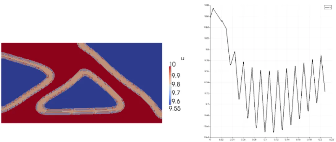
Moreover we present optimal designs for the compliant mechanism problem, which is known to be much harder to solve than the mean compliance problem. It turns out that some compliant mechanism solutions are not reasonable as the interface thickness ap- proaches zero, since no full phase transition is formed. We argue that this is due to the poorly modeled cost functional which does not take a reaction force into account as in [Sig97]. We show numerically that this issue can be solved by introducing a workpiece which exerts a reaction force on the mechanism. However, this reaction force should be part of the model, for which further research is necessary.

Finally a comparison of the obtained optimal designs to the existing literature shows that on the one hand many optimal designs can be recovered by the VMPT method, but on the other hand the VMPT method converges to local minima which cannot be found in the existing literature. Moreover we show that the VMPT method is superior to state-of- the art numerical methods including pseudo time stepping, a reduced SQP method, and a semismooth Newton method, due to its fast and global convergence.

The goals of the thesis can be summarized as follows:

1. Analysis of a new abstract class of numerical methods in Banach space.

2. Discussion of the new method, i.e. special instances of the method, examples and comparison to other methods.

(16)

3. Analysis of a topology optimization problem using a phase field model.

4. Full numerical study of the VMPT method applied to the concrete optimization problem.

5. Numerical study of the topology optimization problem, including parameter choice and aspects of the phase field model.

The thesis is organized as follows.

Section 3 gives an overview of existing numerical methods for constrained optimization in Banach space.

Section 4 contains analysis and discussion of the VMPT method. The new method is derived on the basis of the projected gradient method in Section 4.1, and the algorithm for line search globalization is provided. Section 4.2 facilitates the precise assumptions together with the proof for the well-posedness of the subproblem and for global convergence. In Section 4.3 sufficient conditions for global convergence are discussed, where details for a point based choice of the variable metric are given in Section 4.4. Globaliza- tion along the projection arc is considered in Section 4.6. Only a weak continuity of the projection arc can be shown which does not imply the existence of positive step lengths.

Thus a hybrid method is proposed combining both globalization strategies. In a Hilbert space setting no hybrid method is needed, for which a proof is given. A special instance of the VMPT method, namely the projected Newton’s method, is included in Section 4.7. Global convergence is shown under a weak coercivity assumption on the Hessian, which takes two-norm discrepancies into account. Moreover, q-superlinear convergence rates are established under locally stronger conditions. These rates hold also if j^′ is only semismooth. In Section 4.8 a BFGS update of the variable metric is considered. Global convergence is shown under standard assumptions using an additional small shift of the metric. Section 4.9 contains remarks about the projection type subproblem. In particular a scaling of Barzilai-Borwein type is derived and the inexact solution of the subproblem is discussed. In Section 4.10 the VMPT method is generalized for the minimization of the sum of a differentiable and a convex nonsmooth functional, for which global convergence is established as in the smooth case. Section 4.11 comments on similarities of the VMPT method to other methods in the literature such as pseudo time stepping methods and operator splitting methods. Finally, a concrete application to a semilinear elliptic optimal control problem is presented in Section 4.12, where the problem is posed in the Banach spaceL^∞(Ω) and the VMPT method is carried out with respect to theL²(Ω)-inner product.

Section 5 gives an introduction to general topology optimization. In particular, typical difficulties arising in topology optimization are pointed out and state-of-the-art numerical solvers and models are summarized.

Section 6contains the analysis, discussion and numerics for an abstract class of structural topology optimization problems in linear elasticity using a vector-valued phase field model posed in the Banach space H¹(Ω)^N ∩L^∞(Ω)^N. The abstract problem together with the used assumptions is stated in Section 6.1. Many examples for the abstract data are given.

The special case of two phases is discussed separately, since it can be reduced to a problem using a scalar-valued phase field. Throughout the thesis the analysis is performed for the general vector-valued phase field problem and the results for the scalar-valued phase field are presented as corollaries. Section 6.2 is devoted to the analysis of the control-to-state

(17)

posed and that the state depends locally Lipschitz continuously on the control. Moreover, C²- regularity ofS is shown and the PDEs for the linearized state and the second order derivatives are derived. It is discussed why the analysis is much easier in the Banach space H¹(Ω)^N∩L^∞(Ω)^N than in the Hilbert spaceH¹(Ω)^N. The existence of minimizers for the topology optimization problem in shown in Section 6.3. In Section 6.4 the Γ-convergence result of [BGHR15] is applied to our problem for the scalar-valued case if the boundary traction does not depend on the phase field. Comments on the vector-valued case are given. We establish first order optimality conditions in Section 6.5. The first order derivative of the reduced cost functional is represented by an adjoint approach. Existence and uniqueness of Lagrange multipliers with low regularity is proved. The resulting KKT system is also presented in a strong formulation. The second order derivatives of the reduced cost functional are computed in Section 6.6, again using an adjoint approach.

In Section 6.7 we show that the topology optimization problem fulfills the assumptions for global convergence of the VMPT method. Moreover we introduce six choices for the variable metric, for which we also check the abstract assumptions. The theoretical results for the VMPT method are used in Section 6.8 to propose an adaptive choice for the time step size of pseudo time stepping methods of Allen-Cahn and Cahn-Hilliard type using different time discretizations. Moreover, a rigorous stopping criterion is proposed and global convergence is shown. A reduced SQP method is presented in Section 6.9, which is compared to the VMPT method later on. Section 6.10 contains details about the semismooth Newton (SSN) method and the primal dual active set method, respectively, which are applied to discretized problems with general objective functionals, including the functional of the topology optimization problem and the functional of the projection type subproblem. Local superlinear convergence is shown in case of the VMPT subproblem.

This is also shown for a general objective functional under the assumption of a second order sufficiency condition and strict complementarity. Implementation details are given.

It is shown that applying the SSN method to the unreduced or the reduced problem in case of two phases is equivalent under a certain assumption. Section 6.11 incorporates details about the used discretization of the VMPT method and the adaptive mesh. In Section 6.12 we derive a reasonable scaling parameter λk based on the interface width.

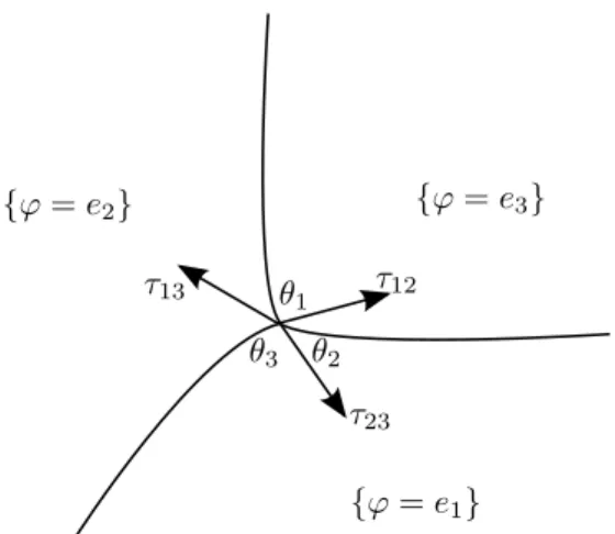
For the used potential the corresponding surface tensions in the sharp interface problem are computed as well as the optimal phase transitions and the angle condition at the triple junctions.

Section 6.13 contains the various numerical results concerning the VMPT method applied to the mean compliance problem. These include results about the used potentials, the interpolation scheme for the stiffness tensors, mesh independency, nesting in the mesh parameter h, the performance of the PDAS method in the inner problem, the behavior of the different choices for the variable metric with respect to computation time and obtained local minimizers, as well as many numerical examples. Moreover, the dependency of the optimal designs and the VMPT method on the model parameters is studied. The obtained optimal designs are compared to existing results in the literature. The adaptiv- ity for the time steps in the pseudo time stepping methods is evaluated numerically and the VMPT method is compared to the resulting method, as well as to the SQP method and the SSN method. Finally, numerical examples for Lagrange multipliers are given and counterexamples for the choice of the variable metric are discussed, which give rise to a mesh dependent VMPT method.

Section 6.14 contains the numerical results about the challenging compliant mechanism problem. As in the preceding section multiple inner products are used to compute the

(18)

optimal designs and a comparison is given. Difficulties for the phase field model in the limit ε → 0 are pointed out on the basis of numerical experiments. It is demonstrated that the obtained local minimizers are undesired and thus a change in the used model is necessary. First numerical examples show that this issue can be circumvented by taking reaction forces into account.

Section 7finally summarizes the new results of this thesis, its implications, and addresses open problems.

(19)

Fr´echet derivatives are denoted by Df or f^′. For functions between finite dimensional spaces this coincides with the Jacobian matrix. By∇f ∶= (Df)^T we denote the transposed Jacobian (the gradient). In particular for real valued functionsDf is a row vector, whereas

∇f is a column vector. We emphasize that we strictly distinguish between the derivative and the gradient. For a real-valued function j in a Hilbert space the gradient∇j is the Riesz representative of the derivative j^′, i.e. ⟨j^′(ϕ), v⟩ = (∇j(ϕ), v) for all v, where ⟨., .⟩ denotes the dual pairing and(., .)the inner product. Sometimes we annotate the space of the dual pairing as index like in ⟨., .⟩_L^∞_,₍_L^∞₎^∗. However, in most cases the space is clear from the context. Usually this will be the abstract spaceX∩Din Section 4 and the concrete spaceH¹(Ω)^N∩L^∞(Ω)^N in Section 6. By∇ ⋅f we denote the divergence of a vector field.

The divergence of a matrix-valued function ∇ ⋅A is defined row-wise and gives a column vector-valued function as result. For partial (Fr´echet-)derivatives we use the notation f_x(x, y) or D_xf(x, y) or ∂₁f(x₁, x₂). In finite dimension we write ∇xf ∶= (D_xf)^T. We denote the space of linear and bounded operators fromX toY by L(X, Y) and identify L(X,L(X, Y))with the space of bilinear continuous mappingsX×X→Y. For the second order Fr´echet derivative we writef^′′. Partial second order derivatives are denoted byf_x,y, where the differentiation with respect tox is applied first. Moreover we use the notation D_x²f ∶= f_x,x, D¹_xf ∶= f_x and D⁰_xf ∶= f. Differentiation directions are placed in square brackets if more than one direction is present, i.e. f_x,y(x, y)[a, b] ∶= (D_y(D_xf))(x, y)ab, where the directionacorresponds toyand the directionbtox. Directions are often named δϕ or τ ϕ, which has to be read as single variable. Vector valued functions are typed in boldface. Set-valued mappings are denoted byF ∶X⇉Y, which is a function from X to the power set ofY. For an introduction in differential calculus we refer to [Zei85].

For 1 ≤ p < ∞ we denote by L^p(Ω) the space of p-integrable functions on Ω (where we identify functions which are equal almost everywhere). The special case L^∞(Ω) is the space of all essentially bounded measurable functions (together with the mentioned identification). We denote by W^k,p(Ω) (=W_p^k(Ω)) the Sobolev space ofp-integrable real- valued functions on Ω with p-integrable weak derivatives up to order k, see also [AF03]

for an introduction to Sobolev spaces. We abbreviateH¹(Ω) ∶=W^1,2(Ω). Sobolev spaces containing vector valued functions are denoted by H¹(Ω,Rⁿ) or in short H¹(Ω)ⁿ. We simply write ∥.∥L² instead of ∥.∥L²(Ω)ⁿ, if the domain and the number of components is clear from the context. If no special qualifier for convergence is given (e.g. weak or weak-

*), then strong convergence is meant. Often the dxis omitted in integral expressions, i.e.

∫Ωf ∶= ∫Ωf(x)dx. We also leave out the space variablex in superposition operators, i.e.

f(ϕ) ∶=f(ϕ(x)) ∶=f(x, ϕ(x))if the meaning is clear from the context.

In the presented estimates, C > 0 is always a generic constant, which can be different from estimate to estimate. We sometimes use H¨older’s inequality∥uv∥L^r ≤ ∥u∥L^p∥v∥L^q for 1/p+1/q=1/r, the trace theorem and obvious inequalities like ∥E(u)∥L² ≤ ∥u∥H¹, where E(u) = ¹₂(Du+Du^T), without reference.

The standard inner product for matrices is denoted by A∶B ∶= ∑ija_ijb_ij, the Euclidean inner product byx⋅y∶= ∑ix_iy_i and the Euclidean norm by∣x∣. Also for matrix and tensor norms and the Lebesgue measure we write ∣A∣, ∣C∣ and ∣Ω∣. Inequalities like ϕ ≥ 0 for vector valued functions are to be understood component-wise and almost everywhere.

We say that a sequence (x_k)k converges q-linearly to zero, if ∣x_k₊₁∣/∣x_k∣ → c for some c∈ (0,1), q-superlinearly, if∣x_k₊₁∣/∣x_k∣ →0 and q-quadratically, if ∣x_k₊₁∣/∣x_k∣²→cfor some c>0.

Since we consider a phase field model in Section 6, the term ‘interface’ always refers to the diffuse interface.

(20)

3 Existing numerical methods for constrained optimization in Banach space

We want to give an overview of state-of-the-art numerical methods for the solution of constrained optimization problems

minj(ϕ), ϕ∈Φad⊂X (4)

posed in a Banach space X. For the Newton-type methods below we will also give the ex- act assumptions for convergence, since we will use these later in the thesis. We emphasize that we cite only results for a Banach space setting. In the case thatX is a Hilbert space or a finite dimensional space much more results are available, of course.

First of all there are Newton-type methods, which are often used due to the typically fast convergence. For constrained optimization the Josephy-Newton method and the semismooth Newton method are appropriate, for which we cite some results which can be found e.g. in [HPUU08]. Both methods don’t solve the optimization problem (4) directly, but are rather based on some optimality condition thereof. Suppose that Φad

is convex. Then a first order necessary condition for a minimizer ϕ is the variational inequality (VI)

ϕ∈Φad, ⟨j^′(ϕ), η−ϕ⟩ ≥0 ∀η∈Φad. (5)

On the other hand, if the admissible set is given by Φad = {ϕ∈X ∣e(ϕ) =0, c(ϕ) ∈ K} for some nonempty convex closed cone K and operators e, c, and if some constraint qualification is satisfied, then a first order necessary condition is given by the KKT system, which involves the primal variable ϕand additional dual variables µ, λ, being Lagrange multipliers for the constraints e(ϕ) =0 andc(ϕ) ∈K, respectively. This KKT system can be written as a generalized equation of the form

0∈G(x) +N(x), (6)

where the unknown xcontains the primal and dual variables,G∶Y →Z is a continuously differentiable operator and N ∶Y ⇉Z is a set-valued map with closed graph. If Φad is nonempty, convex and closed then the variational inequality (5) can also be written as generalized equation with Y =X,Z =X^∗,x=ϕ,G=j^′∶X→X^∗and N =N_Φ_ad∶X⇉X^∗ the normal cone mapping of Φad, i.e.

N_Φ_ad(ϕ) =⎧⎪⎪

⎨⎪⎪⎩

{ξ∈X^∗∣ ⟨ξ, η−ϕ⟩ ≤0 ∀η∈Φad} ϕ∈Φad

∅ ϕ/∈Φad.

The Josephy-Newton method can be used to solve the abstract inclusion (6). In particular the KKT system and the variational inequality (5) can be solved. As for the classical Newton method the algorithm involves successive linearization of the problem. However, since in general only Gis differentiable, the linearization is only applied to Gand not to N. This results in the recursion

0∈G(x_k) + ⟨G^′(x_k), x_k₊₁−x_k⟩ +N(x_k₊₁) (7) for given initialization x0. If the linearized inclusion possesses multiple solutions, then the solution nearest to x_k is taken. For the special case of the VI (5) the Josephy-Newton

(21)

ϕ_k₊₁∈Φad, ⟨j^′(ϕ_k), η−ϕ_k₊₁⟩ +j^′′(ϕ_k)[ϕ_k₊₁−ϕ_k, η−ϕ_k₊₁] ≥0 ∀η∈Φad. (8) The Josephy-Newton method applied to the KKT system results in the SQP method, which calculates in each step a KKT triple(d_k, µ_k₊₁, λ_k₊₁) of the quadratic program

mind ⟨j^′(ϕ_k), d⟩ +1

2Lϕϕ(ϕ_k, µ_k, λ_k)[d, d] (9) e(ϕ_k) +e^′(ϕ_k)d=0 (10) c(ϕ_k) +c^′(ϕ_k)d∈K (11) closest to (0, µk, λk), where L(ϕ, µ, λ) =j(ϕ) + ⟨µ, e(ϕ)⟩ + ⟨λ, c(ϕ)⟩ is the corresponding Lagrange functional. The primal variable is updated byϕ_k₊₁ =ϕ_k+d_k.

Local convergence of the Josephy-Newton method can be shown under the following regularity condition.

Definition 3.1. The generalized equation (6) is said to be strongly regular (in the sense of Robinson [Rob80]) at a solution x^∗ if the perturbed linearized generalized equation is locally uniquely solvable and the solution depends Lipschitz continuously on the pertur- bation, i.e. if there existδ >0, ε>0 and L>0, such that for all p∈Z with ∥p∥ <δ there exists a uniquex(p) ∈Y with∥x(p) −x^∗∥ <εsuch that

p∈G(x^∗) + ⟨G^′(x^∗), x(p) −x^∗⟩ +N(x(p)) and

∥x(p1) −x(p2)∥ ≤L∥p1−p2∥ ∀p1, p2 ∈Z, ∥p1∥ <δ, ∥p2∥ <δ.

The following convergence result can be found verbatim in [HPUU08].

Theorem 3.2. Let Y, Z be Banach spaces, G∶ Y → Z continuously differentiable and let N ∶ Y ⇉ Z be set-valued with closed graph. If x^∗ is a strongly regular solution of the generalized equation (6), then the Josephy-Newton method is locally q-superlinearly convergent in a neighborhood of x^∗. If, in addition, G^′ is γ-H¨older continuous near x^∗, then the order of convergence is 1+γ.

A related method is the semismooth Newton method, which can be used to solve semismooth equations of the form

0=G(x) (12)

for some operatorG∶Y →Z.

Definition 3.3. Let Y, Z be Banach spaces and G∶Y →Z a continuous operator. Let

∂G ∶Y ⇉ L(Y, Z) be given. Then G is called ∂G-semismooth at x ∈Y (in the sense of Ulbrich [Ulb01, Def. 3.1]) if

sup

M∈∂G(x+h)

∥G(x+h) −G(x) −M h∥

∥h∥ →0 as∥h∥ →0.

(22)

G is called ∂G-semismooth of order γ>0 at x∈Y if sup

M∈∂G(x+h)∥G(x+h) −G(x) −M h∥ = O(∥h∥¹⁺^γ) as∥h∥ →0. For examples of semismooth operators we refer to [HPUU08].

The kth semismooth Newton step chooses some operator out of ∂G(x_k) leading to the recursion

0=G(x_k) +M_k(x_k₊₁−x_k) for someM_k∈∂G(x_k) for given x0. The following convergence result is available, see [HPUU08].

Theorem 3.4. LetY,Z be Banach spaces andG∶Y →Z continuous and∂G-semismooth at a solution x^∗ of (12). Let there exist C, δ>0, such that

∥M⁻¹∥ ≤C ∀M ∈∂G(x), x∈Y with ∥x−x^∗∥ <δ.

Then the semismooth Newton method is locally q-superlinearly convergent in a neighbor- hood of x^∗. If G is ∂G-semismooth of order γ >0 at x^∗, then the order of convergence is 1+γ.

In some cases the KKT system can be equivalently reformulated to a semismooth equation of the form (12). This can be done by replacing the complementarity condition in the KKT system by a semismooth projection equation, which is possible e.g. in finite dimension and for pointwise inequality constraints in L². We refer to Section 6.10.1 for an example. The semismooth Newton method can then be used to solve the resulting nonsmooth system.

There is also a Newton type method of Dunn [Dun80], which is not based on an optimality condition. It is similar to the Josephy-Newton method applied to the VI (5). However, an optimization problem corresponding to the linearized VI (8) is solved instead of the linearized VI itself in each Newton step, which is also well defined for non-convex Φad. A drawback of Newton type methods certainly is that convergence is only guaranteed if the initial guess is sufficiently close to the solution. To obtain global convergence additional effort has to be put into globalization strategies such as line search or trust region methods.

We have seen that optimality conditions can be written as an abstract generalized equation (6). Another class of numerical methods for solving generalized equations are operator splitting methods. They consider problems of the form

0∈T(ϕ) (13)

with either T ∶X⇉X or T ∶X ⇉X^∗. For some splitting T =T₁+T₂ the iterates of the method are given by the recursion

1

λ_k(ϕ_k−ϕ_k₊₁) ∈T₁(ϕ_k) +T₂(ϕ_k₊₁),

where λ_k >0 is a step size parameter. We refer to Section 4.11.2 for a detailed discussion. In the context of minimization problems, these methods include the proximal point method (the case T₁ = 0) and the proximal gradient method (the case T₂ = ∂χ_Φ_ad and T =j^′, see Section 4.10). Only few results are available if X is a Banach space compared to the Hilbert space or finite dimensional case. In [Bre09] convergence of a proximal gra-

(23)

operators can be found in [LMMWX12, Cho15]. For the special case of the proximal point method the following results are available in Banach space: In [IB97] convergence is studied for convex optimization problems of the form (4). Convergence analysis for variational inequalities involving maximal monotone operators is covered in [BS00]. Finally a method for the general problem (13) with maximal hypomonotoneT⁻¹ is discussed in [OI07]. Ex- cept for the last reference all mentioned authors assume convexity of the optimization problem or some kind of monotonicity for the generalized equation (13).

Another method for solving constrained optimization problems in Banach spaces are augmented Lagrangian methods. These methods involve the primal and dual variables. Instead of the usual Lagrangian an augmented Lagrangian containing a penalty term is used. However, contrary to penalty methods the penalty parameter is not needed to tend to infinity, since an approximation of the Lagrange multiplier is maintained. As an example consider the case that Φad = {ϕ ∈ X ∣G(ϕ) ∈ K}, for some G ∶ X → H, a Hilbert spaceH and a convex closed cone K⊂H. The augmented Lagrangian then reads

Lc(ϕ, µ) = inf

y∈K−G(ϕ)j(ϕ) − ⟨µ, y⟩ + c 2∥y∥²

with penalty parameterc>0, see [SS04]. Forc=0 the usual Lagrangian is recovered, L(ϕ, µ) =j(ϕ) + ⟨µ, G(ϕ)⟩

if µ ∈ K⁻ ∶= {µ ∈ H^∗ ∣ ⟨µ, ξ⟩ ≤ 0 ∀ξ ∈ K} (dual feasibility). The goal is to compute a solution of the augmented Lagrangian dual problem

sup

µ∈H

ϕinf∈XLc(ϕ, µ), (14)

while the primal problem

ϕinf∈Xsup

µ∈H

Lc(ϕ, µ)

is equivalent to the optimization problem (4) for anyc≥0. In every step of the method, the inner problem of (14) in the primal variable ϕ is solved and the dual variable µ is updated by some strategy, e.g. by a single step of the gradient method applied to the outer problem of (14) as in [IK08]. Moreover, an update rule for the penalty parameter c can be employed. In [BI12] global convergence is shown for an augmented Lagrangian method applied to a general convex optimization problem in a Banach space with pointwise inequality constraints in L^p (i.e. H = L^p and K = {f ∈L^p ∣ f ≤ 0 a.e.}). Therefor it is shown that the augmented Lagrangian method coincides with the proximal point method applied to the unaugmented dual problem

0∈∂_µ(−inf

ϕ∈XL(ϕ, µ) +χ_K⁻(µ)), (15) whereχ_K⁻ is the indicator function ofK⁻,

χ_K⁻(ϕ) =⎧⎪⎪

⎨⎪⎪⎩

0 ϕ∈K⁻

∞ ϕ∉K⁻,

Projection type methods in Banach space with application in topology optimization

application in topology optimization

Contents

3 Existing numerical methods for constrained optimization in Banach space