A duality-based path-following semismooth Newton method for elasto-plastic contact problems

A duality-based

path-following semismooth Newton method for elasto-plastic contact problems

M. Hintermüller^a,∗, S. Rösel^a

aDepartment of Mathematics, Humboldt-Universität zu Berlin, Unter d. Linden 6, D-10099 Berlin, Germany

Abstract

A Fenchel dualization scheme for the one-step time-discretized contact problem of quasi-static elasto-plasticity with combined kinematic-isotropic hardening is considered. The associated path is induced by a coupled Moreau-Yosida / Tichonov regularization of the dual problem. The sequence of solutions to the regularized problems is shown to converge strongly to the optimal displacement- stress-strain triple of the original elasto-plastic contact problem in the space-continuous setting.

This property relies on the density of the intersection of certain convex sets which is shown as well.

It is also argued that the mappings associated with the resulting problems are Newton- or slantly differentiable. Consequently, each regularized subsystem can be solved mesh-independently at a local superlinear rate of convergence. For efficiency purposes, an inexact path-following approach is proposed and a numerical validation of the theoretical results is given.

Keywords: elasto-plastic contact, variational inequality of the 2nd kind, Fenchel duality, Moreau-Yosida/Tichonov regularization, path-following, semismooth Newton

2010 MSC:49M15, 49M29, 74C05, 74S05

1. Introduction

In this paper we consider the quasi-static elasto-plasticity model with an associative flow law (sometimes called Prandtl-Reuss normality law) and von Mises hardening under the small strain assumption set forth in [22]. First investigations of the elasto-plastic problem from a mathematical point of view can be found in [16, 33], where [33] includes existence for the fully continuous case.

Numerical analysis of the semi-discrete and fully-discrete versions can be found, for example, in [2, 22]. Appropriate discretization schemes for plasticity problems with hardening have been in- vestigated extensively in the recent past. Here we only mention [3, 10, 9, 43] for adaptive finite element methods. Concerning numerical solution methods, we refer to the multigrid approach in [47], various generalized Newton methods in finite dimensions [12, 20, 42, 47, 48], including the standard return mapping algorithm in [44] as well as interior point strategies, cf. e.g. [37].

A general introduction to elastic contact problems including corresponding numerical approaches can be found in the monographs [31, 41], and multigrid methods for elastic contact are analyzed, e.g.,

∗Corresponding author, phone: +49 (0)30 2093-2668

Email addresses: hint@math.hu-berlin.de(M. Hintermüller),roesel@math.hu-berlin.de(S. Rösel)

Preprint submitted to Elsevier

Published in: Journal of Computational and Applied Mathematics 292 (2016) 150–173

April 10, 2015

in [35] and [36, 38], where the latter references are devoted to two-body contact. For the treatment of elastic friction problems we refer to [13, 38] as well as to the efficient active set algorithm proposed in [32]. Subspace correction methods for variational inequalities of the second kind with application to frictional contact have been investigated in [5]. In [12, 21] plastic material behavior is incorporated in addition to the contact constraints. In the latter references the elasto-plastic friction problem is reformulated utilizing a nonlinear complementarity problem (NCP) function yielding a nonsmooth system which can be solved efficiently by applying a generalized Newton method in a discrete framework provided a set of damping parameters is chosen appropriately.

While some attention has been paid to infinite-dimensional methods in linear elasticity with (frictional) contact [39, 45], elasto-plastic problems are still less researched. Among the few available references we mention [8] for domain decomposition methods leading to a linear rate of convergence.

The approach to plasticity problems without contact constraints in [20], however, turns out to be problematic as far as function space convergence of the employed semismooth Newton (SSN) solver is concerned. In fact, due to the lack of a sufficient norm gap between domain and image space of the mapping involved in the underlying nonsmooth system, generalized differentiability in the sense of [30] does not hold true. The resulting lack of a well-defined infinite-dimensional generalized Newton iteration usually results in a mesh-dependent solver.

In the present paper, we introduce a path-following semismooth Newton method which admits a rigorous convergence analysis in the continuous setting. For this purpose, we study a regu- larized version of the Fenchel-dual problem of the underlying elasto-plastic contact problem with the regularization parameter inducing a dual path to the solution of the original problem. Each path-problem can be solved at a local superlinear rate and in a mesh-independent way upon dis- cretization.

2. Problem formulation

The starting point of our analysis is the small-strain elasto-plastic contact problem in the dis- placementu, the plastic strainpand a set of internal variablesξwhich model the evolution of a body subject to given applied forces. The body is represented by a bounded domainΩ⊂R^N, N= 2,3, withN^0,1-property [49] and it adheres to a fixed partΓd ⊂∂Ωwith positive surface measure. We further denote byΓn⊂∂Ω\Γdsome relatively open part of the boundary where a given surface load g∈L²(Γn)is applied. A given volume force density is denoted byf ∈L²(Ω). The elasto-plastic behavior at a material pointx∈Ωis determined by a given yield criterion leading to a dissipation functional which typically is nonsmooth, lower semicontinuous (l.s.c.) and convex [22]. Often, the displacement of the body is restricted by a given rigid obstacle giving rise to an elasto-plastic con- tact problem. Therefore we fix a setΓ_c⊂∂Ωwhich potentially contains the contact region with the obstacle. We emphasize here that the approach presented in this work does not hinge onΓ_c 6=∅.

To measure the gap betweenΩand the obstacle we use a given function ψ∈Z:=H^1/2(Γc)withψ≥0almost everywhere (a.e.) onΓc;

see [41]. For the time being we neglect frictional forces such that in terms of the variational formulation, we incorporate the contact constraint by a kinematic non-penetration condition on the displacementu:

τnu≤ψonΓc, (2.1)

whereτn: [H_0,Γ¹

d(Ω)]^N →Z, u7→(τ|Γ_c(u))·ndenotes the normal trace mapping restricted toΓc. For analytical reasons we assume thatΓc is relatively open withN^1,1-property and C^∞-boundary

∂Γc. For simplicity and without loss of generality we further stipulate

Γc ⊂Σ, (2.2)

whereΣdenotes the interior of∂Ω\Γdin∂Ω, to avoid working with the spaceH₀₀^1/2(Γc). Concerning the splitting of the boundary we further assume

∂Ω = Γc∪Γn∪Γd, Γc∩Γn∩Γd=∅, ∂Σ∈C^∞.

To formulate the quasi-static problem, we first fix the notation which is loosely based on the monograph by Han and Reddy [23]. We endow the Hilbert spaces

V := [H_0,Γ¹

d(Ω)]^N, Q:= [L²(Ω)]^N×N_sym

with the usual scalar products. In this context, C(x)∈R^N×N×N×N,Cijkl ∈L^∞(Ω), denotes the fourth-order elasticity tensor which is assumed to be symmetric, i.e. Cijkl = Cklij = Cjikl and pointwise stable, i.e. ∃C >0with

C(x)σ:σ≥C|σ|²_F ∀σ∈R^N_sym^×N and a.e. x∈Ω, where A : B = P

i,j=1...Naij ·bij for A, B ∈ R^N×N. Analogous properties are supposed to be fulfilled by the hardening modulusH(x)∈R^m×m. The symmetric part of the displacement gradient is denoted byε(u), i.e.,

ε(u)(x) =¹₂(∇u(x) +∇u(x)^>).

Further, tr(σ) := ^PN_i=1σii stands for the matrix trace operator. The plastic incompressibility con- dition onpgives rise to the closed subspaceQ0ofQdefined by

Q0:={q∈[L²(Ω)]^N_sym^×N : tr(q) = 0a.e. inΩ}

which inherits the scalar product ofQ.

Quasi-static elasto-plastic contact problem. Given some material-dependent l.s.c., convex and proper yield functionalφ : R^N_sym^×N ×R^m → R∪ {+∞}, the underlying elasto-plastic contact problem with a linear hardening law consists of seeking(u, p, ξ)(t)∈V ×Q₀×L²(Ω)^m, t∈[0, T], with(u, p, ξ)(0) = 0, such that

u= 0 onΓ_d, (2.3)

σn=g onΓn, (2.4)

divσ=−f, (2.5)

ε(u) =C⁻¹σ+p, (2.6)

(σ,−Hξ)∈K:={(˜σ,χ) :˜ φ(˜σ,χ)˜ ≤0}, (2.7)

( ˙p,ξ)˙ ∈NK(σ,−Hξ), (2.8)

τ_Tσ= 0, τ_nnσ≤0, τ_nnσ(τ_nu−ψ) = 0, τ_nu≤ψ onΓ_c, (2.9)

for a.e. t∈[0, T], where N_K(˜σ,χ)˜ denotes the normal cone to the convex setKat (˜σ,χ). Further-˜ more,τnnσ:= (τnσ)^>n, and τTσ:=τnσ−(τnnσ)n denotes the tangential trace onΓc, and( ˙p,ξ)˙ represent the derivative in time. Note that (2.6)-(2.8) determine the plasticity behavior and (2.9) represents the complementarity conditions of contact; for details cf. [23, 41].

Incremental formulation. An implicit Euler discretization of the time derivatives appearing in the associative flow law (2.8) leads to the following weak form of the incremental problem:

(min J˜(u, p, ξ) over(u, p, ξ)∈V ×Q×L²(Ω)^m

subject to (s.t.) τ_nu≤ψonΓ_c, (2.10)

with

J˜(u, p, ξ) := ¹₂ Z

Ω

C(ε(u)−p) : (ε(u)−p) +ξ:Hξdx +

Z

Ω

χ^∗_K(p−p0, ξ−ξ0) dx

− Z

Ω

f·udx− Z

Γ_n

g·udx,

whereχ^∗_K denotes the convex conjugate of the characteristic functionχK of the convex setK and p0, ξ0 denote the states of the variables from the preceding time instance.

Combined linearly isotropic-kinematic hardening with the von Mises yield condi- tion. For combined isotropic-kinematic hardening it holds that ξ= [p, η]∈ R^n×n₀ ×R, H(p, η) = k1p+k2η withk1, k2≥0, and the associated von Mises yield function is defined by

φ(σ,[a, g]) :=|devσ+a|_F+g−σ_y+χ_R−

0(g), [a, g]∈R^n×n₀ ×R, (2.11) with some material-dependent yield stressσy >0, cf. [23]. In this case, a variable shift replacing (p−p0)bypin (2.10), leads to the problem

(min J(u, p) over(u, p)∈V ×Q₀ s.t. τnu≤ψonΓc

(2.12) with

J(u, p) := ¹₂ Z

Ω

C(ε(u)−p) : (ε(u)−p) + ¯k p:pdx + Z

Ω

β|p|_Fdx +l(u, p),

whereβ= (σ_y+k₂η₀)∈L²(Ω)withβ≥σ_ya.e. inΩ,¯k= (k₁+k₂)∈L²(Ω), and a linear functional l(u, p) :=−

Z

Γn

guds− Z

Ω

f u+k1p0:p− C(ε(u)−p) :p0dx,

with l ∈ (V ×Q0)^∗, the topological dual space to V ×Q0. Note that (2.12) is equivalent to an elliptic variational inequality of the mixed (i.e. first and second) kind. Writing

y:= (u, p)∈Y :=V ×Q0, p=: Π_Q0(u, p), Π_Q0∈ L(Y, Q0), a([u, p],[˜u,p]) :=˜

Z

Ω

C(ε(u)−p) : (ε(˜u)−p) + ¯˜ k p: ˜pdx,

yields a more compact form ofJ :Y →R:

J(y) = ¹₂hAy, yi(Y∗,Y)+l(y) + Z

Ω

β· |ΠQ0y|Fdx, (EP)

where A ∈ L(Y, Y^∗) is the linear and continuous operator from Y to its topological dual Y^∗ associated to the bilinear form a : Y ×Y → R. We note that a is Y-elliptic if essinfΩ¯k > 0, cf. [22]. Standard arguments then show that (2.12) admits a unique solution y¯ = (¯u,p)¯ ∈ Y. The condition onk¯ is always supposed to be fulfilled, otherwise we would leave the framework of hardening plasticity for a problem of perfect plasticity which requires a different functional analytic setting, cf. [14]. However, the resulting problem may be approximated consistently by a sequence of plasticity problems with vanishing hardening [6].

Remark. Using Moreau’s theorem, (EP) can be further reduced to a (Fréchet) differentiable problem in the displacement only, cf. [20]. However, the resulting optimality condition is not el- igible to Newton differentiation (in the sense of [30]) in infinite dimensions which may result in mesh-dependent convergence of an associated generalized Newton scheme. While the Newton dif- ferentiability of the stationarity system is always given in finite dimensions, the spatially continuous case requires a certain norm gap which is indispensable for the Newton differentiation of the in- volved composedmax-function, cf. [27, 28] or section 6 for related issues. Such an integrability gap can never be achieved without further regularization.

3. Fenchel duality for the elasto-plastic contact problem

For numerical purposes it turns out that the Fenchel dual problem to (2.12) is favorable in the sense that, upon regularization, it can be solved efficiently by semismooth Newton techniques.

In order to establish a compact set-up for the application of the Fenchel duality theory, the elasto-plastic contact problem (2.12) will be rewritten in the form

minF(y) +G(Λy), overy∈Y, (EPC)

with a Gâteaux-differentiable functionF, a l.s.c., proper, and convex functionGand a linear and continuous operatorΛ. In fact, we defineF :Y →Rby

F(y) := ¹₂hAy, yi(Y∗,Y)+l(y).

Further, we denote the convex cone associated to the constraint (2.1) by K₁:={z∈Z:z≤0 a.e. onΓ_c}

and defineG:Z×L²(Ω)^d→R∪ {+∞} by G(z, q) :=G₁(z) +G₂(q) :=χ_ψ+K1(z) +

Z

Ω

β|q|2dx. Moreover, we set

Λ :=

τn 0 0 M^1/2P⁻¹

∈ L(Y, Z×L²(Ω)^d),

whereχψ+K₁ is the indicator function of the set ψ+K1, and P : (L²(Ω)^d,k.k_{L2 (Ω)}d)→(Q₀,k.kQ0),

withd=^N(N₂⁺¹⁾−1, denotes the canonical parametrization given by

[q1, q2]7→^P

q1 q2

q2 −q1

; [q1, q2, q3, q4, q5]7→^P





q1 q3 q4

q3 q2 q5

q4 q5 −(q1+q2)



; (3.1)

forN= 2,3, respectively. The symmetric positive definite matrixM is defined by M =

2 0 0 2

; M =





2 1 0 1 2 0 0 0 2



;

forn= 2,3, respectively, such thatP p:P q=M p·q ∀p, q∈R^d.

This setting differs from the one presented in [45] mainly by the choice of the operatorΛ which entails a slightly different interpretation of the dual variableq, cf. (3.8). We next compute and analyze the dual problem to (EPC).

Computation of the Fenchel conjugates. The convex conjugateF^∗:Y^∗→RofF :Y →R is given by

F^∗(y^∗) = ¹₂hy^∗−l, A⁻¹(y^∗−l)i(Y∗,Y). For the nondifferentiable partGwe obtain

G^∗:Z^∗×L²(Ω)^d→R∪ {+∞}, G^∗(z^∗, q) =G^∗₁(z^∗) +G^∗₂(q), with

G^∗₂:L²(Ω)^d →R∪ {+∞}, G^∗₂(q) =χK2(q), whereK2:={q∈L²(Ω)^d:|q|2≤β a.e. in Ω}, and

G^∗₁:Z^∗→R∪ {+∞}, G^∗₁(z^∗) = sup

z∈K1+ψ

hz^∗, zi=χ_K^∗

1(z^∗) +hz^∗, ψi, where it is understood that

K₁^∗:=Z₊^∗ ={z^∗∈Z^∗:z^∗≥0}

={z^∗∈Z^∗:hz^∗, zi ≥0 ∀z∈Z withz≥0 a.e. onΓ_c}. (3.2) The dual problem to (EPC) is given by

sup −F^∗(−Λ^∗[z^∗, q])−G^∗(z^∗, q) over[z^∗, q]∈Z^∗×L²(Ω)^d, (D) which can be equivalently expressed as







−inf F^∗(Λ^∗[z^∗, q])− hz^∗, ψi over[z^∗, q]∈Z^∗×L²(Ω)^d s.t. z^∗≤0,

|q|2≤β a.e. inΩ.

Note the sign change in the dual variables and that the first inequality constraint has to be under- stood in the sense of (3.2).

SinceK1+ψhas empty interior, a generalized Slater condition fails to hold. Hence the Fenchel duality theorem in its usual version [17] is not applicable. However, in our special situation we are still able to preclude the presence of a duality gap.

Proposition 3.1(Duality). There is no duality gap, i.e. it holds that inf(EPC)= sup(D).

Moreover, there exists a unique solution(¯z,q)¯ ∈Z^∗×L²(Ω)^d to the dual problem.

Proof. We make use of [4, Theorem 1, Chapter 4.6], and need to show that

0∈int (Λ^∗domG^∗+ domF^∗). (3.3)

As F^∗ is finite everywhere, we have domF^∗ = Y^∗. Further, domG^∗ 6= ∅ implies Λ^∗domG^∗ + domF^∗=Y^∗ such that (3.3) is always satisfied. It follows that no duality gap occurs.

Regarding existence and uniqueness of a solution to (D) we notice that the objective function is continuous and strictly convex sinceF^∗ is strongly convex andΛ^∗is injective by the surjectivity of τn, cf. (2.2). Moreover, coercivity of the objective function follows from ellipticity of the bilinear form associated to A⁻¹. Indeed, with κ > 0 denoting the corresponding ellipticity constant, it follows that

F^∗(Λ^∗[z^∗, q])− hz^∗, ψi

= ¹₂hΛ^∗[z^∗, q]−l, A⁻¹(Λ^∗[z^∗, q]−l)i(Y∗,Y)− hz^∗, ψi

≥ ^κ₂kΛ^∗[z^∗, q]k²_Y∗− kΛA⁻¹l+ [ψ,0]kk[z^∗, q]k_{Z∗ ×L2 (Ω)}d+^κ₂klk²

≥ _2kΛ^κ−∗k²k[z^∗, q]k²_{Z∗ ×L2 (Ω)}d− kΛA⁻¹l+ [ψ,0]kk[z^∗, q]kZ∗ ×L2 (Ω)d+^κ₂klk²,

where the last estimate follows from the fact thatΛ^∗ has a bounded inverse on its (closed) range owing to the closed range theorem.

Optimality conditions. By the absence of a duality gap (Proposition 3.1), the solution

¯

y= [¯u,p]¯ of the primal problem (EPC) can be recovered from the solution [¯z,q]¯ of (D) from

Λ^∗[¯z,q] =¯ A¯y+l, (P-D)

−[¯z,q]¯ ∈∂G(Λ¯y).

Due to (3.3), we may characterize the solution [¯z,q]¯ ∈ Z^∗×L²(Ω)^d by the existence of ¯λ = [¯µ,ν¯]∈Z×L²(Ω)^d satisfying

ΛA⁻¹Λ^∗[¯z,q]¯ −ΛA⁻¹l−[ψ,0] + ¯λ= 0, (OC1)

¯

z≤0,|¯q|2≤β a.e. in Ω, (OC2)

h¯µ, z^∗−zi ≤¯ 0, (¯ν, q−q)¯ ≤0 ∀z^∗≤0, ∀ |q|2≤β a.e. in Ω, (OC3)

where the (OC3) expresses thatλ¯ is an element of the normal cone to−K₁^∗×K2 at[¯z,q]. Equiva-¯ lently, there exists[¯µ,ζ]¯ ∈Z×L²(Ω)with

ΛA⁻¹Λ^∗[¯z,q]¯ −ΛA⁻¹l−[ψ,0] + [¯µ,ζ¯q] = 0,¯ (3.4)

ζ¯−max(0,ζ¯+c(|¯q|2−β)) = 0, c >0, (3.5)

¯

z≤0, (3.6)

h¯µ, z^∗−zi ≤¯ 0 ∀z^∗≤0. (3.7)

In general, these conditions are not directly eligible to the semismooth Newton method in the sense of [30]: Firstly, for generalized differentiation of the mapping associated with the left hand side of (3.5) in infinite dimensions, the setting lacks a suitable norm gap, see [27, 28] and section 6. Note that these issues are absent if a direct discretization is applied which may, however, be at the cost of mesh dependent convergence rates.

Secondly, (3.7) cannot be reformulated with the help of a pointwise NCP-function, i.e., a function φ:R²→Rwith the property

a≥0, b≥0, ab= 0⇐⇒φ(a, b) = 0.

This is due to the fact that elements ofZ^∗ in general do not allow for a pointwise interpretation.

For these reasons we employ a penalization-regularization approach in the next sections.

Interpretation of the dual variables. Considering the second component in (P-D) and using P^∗=M P⁻¹, we obtain a direct relation betweenq¯and the optimal stress¯σ:=C(ε(¯u)−p):¯

P(M^−1/2q) =¯ −¯σ+ ¯k¯p+k1p0+Cp0 inQ^∗₀. This implies

P(M^−1/2q) =¯ −dev(¯σ−Cp0) +k1(¯p+p0) +k2p¯ inQ0, (3.8) which shows that|q|¯2−σycorresponds to the value of the von Mises yield function, cf. (2.11). Thus, the norm ofq¯determines the elasto-plastic material behavior. Moreover, by multiplying (P-D) by [u,0], u∈ V, it may be shown, analogously to the elastic case [41, 45], thatz¯ corresponds to the normal stressτnnσ¯ ∈Z^∗ at the contact boundary.

4. Regularization

In order to render the optimality conditions (OC1-3) amenable to the semismooth Newton method we now choose a Hilbert subspaceH =H1×H2⊂L²(Γc)×L²(Ω)^d with dense embedding

H =H1×H2,→Z^∗×L²(Ω)^d.

To obtain a consistent regularization,H₁ andH₂are required to satisfy the following properties.

Assumption 4.1(Density of convex intersections). The following density assertions are supposed to hold:

ι^∗₁({z∈H₁:z≤0 a.e. onΓ_c})^Z

∗

=Z₋^∗, {q∈H2:|q|2≤β a.e. inΩ}^{L2 (Ω)}

d

={q∈L²(Ω)^d:|q|2≤β a.e. inΩ}, whereZ₋^∗ :={z^∗∈Z^∗:hz^∗, zi(Z∗,Z)≤0 ∀z≥0}andι^∗₁ is given by (4.1).

We further defineL²:=L²(Γc)×L²(Ω)^d and denote by ι^∗= [ι^∗₁, ι^∗₂] :L²,→[Z×L²(Ω)^d]^∗'Z^∗×L²(Ω)^d the canonical injection

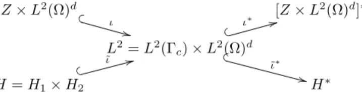
[z, q]7→[(z, .)L2 (Γc)|Z, q] ∈[Z×L²(Ω)^d]^∗. (4.1) Moreover, in the following illustration (see Figure 1) of the embedding framework including two Gelfand triples, we also specify the canonical injection

˜

ι:H →L²,[z, q]7→^˜ι [z, q].

In this section onlyιandι^∗will be mentioned explicitly whereas the other injections are employed

Z×L²(Ω)^d x _ι

++

[Z×L²(Ω)^d]^∗ L²=L²(Γ_c)×L²(Ω)^d

& ^ι∗ 33

y

˜ ι^∗

++H =H1×H2

% ^˜ι 33

H^∗

Figure 1: Gelfand triple framework for the regularization

tacitly. Suitable choices forH₁and H₂ with regard to Assumption4.1, possibly depending on the smoothness ofΓ_c, can be made using Lemmas5.3 and5.4 as well as Lemma5.5of the subsequent section. For specific examples, we refer to section 7 below.

For algorithmic reasons it may be advantageous to include a non-negative shift parameter (ˆµ,ˆν)∈H₊^1/2(Γc)×L^∞₊(Ω),

see [26]. Finally we replaceβ by anL^∞-approximationβγ which shall satisfy σy≤βγ ≤β a.e., ||βγ−β||_{L2 (Ω)}≤ ¹_γ

for allγ.

Regularized problem. Following [15] we consider the regularized problem:

minJ_γ^∗(z, q) over[z, q]∈H (D_γ)

with

J_γ^∗(z, q) :=F^∗(Λ^∗ι^∗[z, q])−(z, ψ)_{L2 (Γc)}+M_γ¹(z) +M_γ²(q) +Tγ(z, q),

where we employ the following Moreau-Yosida-type regularizations of the indicator function asso- ciated with the inequality constraints in (D):

M_γ¹(z) := _2γ¹ k[ˆµ+γz]⁺k²_L2(Γc),

M_γ²(q) := _2γ¹ k[ˆν+γ(|q|2−βγ)]⁺k²_L2(Ω),

as well as a regularization term of Tichonov type:

T_γ([z, q]) := _2γ¹ b([z, q],[z, q]), (4.2)

where b : H ×H → R is a continuous and coercive bilinear form represented by the operator B∈ L(H, H^∗)with ellipticity constantκb>0.

Optimality condition. Note that (Dγ) has a unique solution v_γ = [z_γ, q_γ] ∈ H which is characterized by

0 =Nγvγ−ιwˆ+ ([µγ, νγ], . )L2 in H^∗ (OC1γ) with





 ˆ

w= [ˆz,q] = ΛAˆ ⁻¹l+ [ψ,0], µ_γ = [ˆµ+γz_γ]⁺ ∈L²(Γ_c),

νγ = [ˆν+γ(|qγ|2−βγ)]⁺q(qγ)∈L²(Ω)^d,

(OC2γ)

where we defineq(.) :L²(Ω)^d→L²(Ω)^d by q(v) :=

( _v

|v|2 if|v|2>0, 0 else.

Furthermore, the homeomorphismNγ ∈ L(H, H^∗)is defined as N_γ :=ιΛA⁻¹Λ^∗ι^∗+_γ¹B.

We close this section with an important consistency result concerningγ→+∞. This result suggests a path-following-type approach, where the associated primal-dual-path is induced by a sequence (γ_k)withγ_k >0.

Theorem 4.2(Convergence of regularized dual solutions). Let(γ)⊂R⁺, γ→ ∞. Under Assump- tion4.1 it holds that

(i) vγ = [zγ, qγ]*[¯z,q]¯ inZ^∗×L²(Ω)^d, (ii) λγ = [µγ, νγ]*[¯µ,ν]¯ inH₁^∗×H₂^∗, and

Λ^∗ι^∗v_γ →Λ^∗[¯z,q]¯ inY^∗. Proof. See appendix Appendix A.

As a simple consequence of the previous theorem, the sequence of approximations of the optimal displacement-strain pair and the sequence of trial stresses converge strongly to the corresponding solution of the original elasto-plastic contact problem (EPC). It may further by inferred that the sequence(q_γ)converges even with respect to the norm topology inL²(Ω)^d.

Corollary 4.3(Convergence of primal solutions). Under Assumption4.1, the following assertions hold true:

(i) Foryγ :=A⁻¹(Λ^∗ι^∗[zγ, qγ]−l) it holds thatyγ→y¯ inY. (ii) For σγ :=C(ε(uγ)−pγ)it holds that σγ→σ¯ inQ.

(iii) It holds thatqγ→q¯inL²(Ω)^d. Proof.

(i) The statement follows from the continuity of the operatorA.

(ii) The assertion follows from (i).

(iii) The assertion follows from (i) and the fact thatΛ^∗₂ is a topological isomorphism.

5. Auxiliary results on density-invariant convex intersections

In this section we discuss several conditions which lead to suitable options for the regularization space H with regard to Assumption 4.1. In general, for a Banach space V, an arbitrary dense subsetU ⊂V as well as a convex and closed subset K⊂V the inclusion

K∩U ⊂K∩V (5.1)

is not necessarily dense even for linear subspacesKandU. Therefore we investigate several situa- tions relevant for our application in which the density of inclusion (5.1) is guaranteed. Readers who are merely interested in numerical aspects may as well directly consult the options forH specified in section 7 and take the Assumption4.1for granted.

Lemma 5.1 (intersection-invariant dense embedding). Let V be a Hilbert space and U a dense subsetU ⊂V. LetK⊂V be nonempty, convex and closed. If the projection mappingPK :V →K isU-invariant, i.e.

P_K(U)⊂U,

thenU∩K^V =K, i.e. U∩K is dense in K with respect to the norm inV.

Proof. Forv∈K there exists a sequence(un)⊂U withun →v. Now,PK(un)∈U for alln by assumption, such that

kP_K(u_n)−vk_V =kP_K(u_n)−P_K(v)k_V ≤ ku_n−vk_V →0.

Lemma 5.2 (superposition and trace). Let θ : R→ R be Lipschitz continuous and assume that θ⁰(t)exists except for finitely many points t∈R. Further letΩbe a Lipschitz domain. Assume that µ(Ω)<+∞orθ(0) = 0. For the trace operator τ:H¹(Ω)→H^1/2(∂Ω)it holds that

(θ◦τ)(u) = (τ◦θ)(u) inL²(∂Ω) (5.2)

for allu∈H¹(Ω).

Proof. Under the above conditions, the superposition θ1=θ:L²(∂Ω)→L²(∂Ω)

is well-defined and continuous. Further, it is well known that the superposition θ2=θ:H¹(Ω)→H¹(Ω)

is also well-defined [34] and continuous, cf. [40]. Since (5.2) holds for any u∈ C(Ω)∩H¹(Ω), a density argument completes the proof.

Lemma 5.3. ForL²₋(Γ_c) :={z∈L²(Γ_c) :z≤0 a.e. onΓ_c}it holds that ι^∗₁(L²₋(Γc))^Z

∗

=Z₋^∗.

Proof. Define the closed, convex and nonempty setM ⊂Z^∗ by M :=ι^∗₁(L²₋(Γ_c))^Z

∗

⊂Z₋^∗

and assume Z₋^∗ \M 6= ∅. For 0 6= z^∗ ∈ Z₋^∗ \M it holds that αz^∗ ∈ Z₋^∗ \M for all α > 0.

Furthermore, there exists a sequence(v_n)⊂L²(Γ_c)with

vn →z^∗ in Z^∗. (5.3)

We first assume that ||vn||_{L2 (Γc)} →+∞as n →+∞. The Hahn-Banach Separation Theorem implies that for alln∈Nthere exists zn∈Z with

hzn,_||v ¹

n||²

L2 (Γc)

z^∗i(Z,Z∗)>1 and (5.4)

hzn, vi(Z,Z∗)≤1 for allv∈M. (5.5)

We decompose zn = z_n⁺+z⁻_n into a positive part z⁺_n := max(0, z) and a negative part z⁻_n :=

min(0, z), where it is easy to see that {z_n⁺, z_n⁻} ⊂ Z. Indeed, recall (cf. e.g. [19, p.20]) that Z=H^1/2(Γc)is defined by the set of allz∈L²(Γc)with finite seminorm

|z|²_Γ

c ,1/2:=

Z

Γ_c

Z

Γ_c

|z(x)−z(y)|²

|x−y|ⁿ dx dy<+∞.

Further observe thatmax(0, z)∈L²(Γc)and superposition with Lipschitz functions preserves the finiteness of the seminorm. Alternatively one may invoke Lemma5.2. From (5.4) andz^∗ ∈Z₋^∗ it follows that

hz⁻_n,_||v ¹

n||²

L2 (Γc)

z^∗i(Z,Z∗)>1,

in particularz_n⁻6= 0. Settingv=ι^∗₁(z⁻_n)||z_n⁻||Z||z_n⁻||⁻²_{L2 (Γ}

c) in (5.5), wherev∈M by definition, one obtains

hzn, vi(Z,Z∗)=||z_n⁻||Z≤1. (5.6)

On the other hand, forvn according to (5.3) and for sufficiently largen∈Nit holds that

||z_n⁻||_{L2 (Γc)}= sup

v∈L²(Γ_c)

(z_n⁻,v)_{L2 (Γc)}

||v||_{L2 (Γc)}

≥ ^(z

− n,v_n)_{L2 (Γ}

c)

||v_n||_{L2 (Γ}

c)

= ^hz

−

n,z^∗i_(Z,Z∗)

||v_n||_{L2 (Γ}

c)

−^hz

−

n,z^∗−ι^∗₁v_ni_(Z,Z∗)

||v_n||_{L2 (Γ}

c)

≥ ||vn||_{L2 (Γc)}−^||zn−||_||v^{Z||z∗−ι∗1vn||Z∗}

n||_{L2 (Γc)}

→+∞ forn→+∞,

due to (5.3) and (5.6). This clearly contradicts (5.6).

If(v_n)is bounded inL²(Γ_c), it converges weakly (along a subsequence) inL²(Γ_c)to an element u∈L²(Γc), such thatz^∗=uby (5.3). This in turn impliesz^∗∈L²(Γc)∩Z₋^∗ =L²₋(Γc). The latter equation relies on the density ofZ+in L²₊(Γc)with respect to the norm topology inL²(Γc), which holds as a consequence of Lemma 5.1. Thus it holds that z^∗ ∈ M, which contradicts the initial hypothesis.

Lemma 5.4. Let Ω⊂Rⁿ be open, µ(Ω)<+∞,d∈Nandβ: Ω→Rmeasurable withβ(x)≥σ >

0 a.e. inΩ. For

K:={u∈L²(Ω)^d :|u|2≤β a.e. inΩ}

it holds thatK_∞:=K∩[C₀^∞(Ω)]^d is densely contained inK, i.e. K_∞^{L2 (Ω)d}=K.

Proof. Letu∈K andε >0.

Part I. We first choose a functiong∈C₀⁰(Ω)^d, g= [g1, . . . , gd], with the following properties:

(|gj(x)| ≤ |uj(x)| a.e. in Ω,

||gj−uj||_L2(Ω) < ^√ε

d, (5.7)

forj= 1, . . . , d. A suitable choice can be made using Lusin’s Theorem: In fact, there exist for all δ >0

Kj⊂Ωcompact, µ(Ω\Kj)< δ, j= 1, . . . , d, withuj |K_j continuous. We define theC₀⁰(Ω)-functions

g_j(x) := min(δ,dist(x,Ω\Kj))

δ u_j(x)

which fulfill (5.7) for sufficiently smallδ.

Thereforeg∈C₀⁰(Ω)^d is an element ofK. Moreover, kg−uk²_L2(Ω)^d =

d

X

j=1

||gj−uj||²_L2(Ω)< ε².

We thus have shown thatK0:=K∩C₀⁰(Ω)^d is densely contained inK.

Part II. To conclude the proof we take an arbitrary sequence(un)_n∈N⊂K0 which fulfills

||un−u||_L2(Ω)^d→0.

Further setu˜_n:= _n+1ⁿ u_n∈C₀⁰(Ω)^d.

By continuity and the hypothesisβ(x)≥σa.e. in Ωthere existsδ_n>0with

|˜un|2(x)≤β(x)−δn for a.e. x∈Ω. (5.8)

Moreover, for everyna suitable mollification yields a sequence(v^k_n)_k∈N ⊂[C₀^∞(Ω)]^d with lim

k v^k_n→u˜n inC( ¯Ω). (5.9)

Combining (5.8) and the uniform convergence property (5.9) one obtains that for eachnthere exists k(n)such thatv^k_n∈K_∞ andkv_n^k−u˜_nk_{L2 (Ω)}d< ^ε₃ for allk≥k(n).

Finally choosensufficiently large such that ku−unk_{L2 (Ω)}d<₃^ε, kun−u˜nk_{L2 (Ω)}d<₃^ε.

Applying the triangle inequality shows that(v^k(n)n )⊂K∞satisfies kv^k(n)_n −uk_L2(Ω)^d< ε,

for sufficiently largen, which accomplishes the proof.

The contact boundary as a Riemannian manifold. In order to allow for a distribution theory on the manifoldΓ_csimilar to the Euclidean case, we need to define the space of test functions C₀^∞(Γ_c) on a manifold Γ_c which requires a smooth structure. In connection with an associated Riemannian measure this leads to the definition of Sobolev spaces on manifolds allowing for a complete calculus theory, cf. [18]. For the alternative approach via the completion of smooth functions w.r.t. theW^k,p-norm see [24].

In the remaining part of this section we therefore assume that the contact boundaryΓcis smooth, i.e., aC^∞-submanifold of Rⁿ. More precisely, since∂Ωis assumed to have theN^0,1-property [49],

∂Ω (possibly after an appropriate orthogonal coordinate transformation) is given locally by the graph of functions αi ∈C_B^0,1, i= 1, . . . , m. We assume that those αi whose graph has nonempty intersection withΓc, are not only inC_B^1,1 but inC^∞∩C_B^1,1 on an appropriate bounded domain in R^N−1. Here, the space C_B^k,κ is defined as the set ofk-times continuously differentiable functions with bounded derivatives of order less than or equalkandκ-Hölder-continuousk-th derivative [49].

In this way,Γcbecomes an(N−1)-dimensionalC^∞-submanifold ofR^N. We further endow the Cartesian product of the tangent spaces ofΓc with the usual scalar product inR^N. This canonical construction yields a Riemannian manifold(Γc,h. , .i_RN).

Lemma 5.5. Let Γc be aC^∞-submanifold ofR^N and consider(Γc, g),g=h. , .i_RN, as a Rieman- nian manifold with associated Riemannian measure µ=µ(g). Then for L²₋(Γc) :={u∈L²(Γc) : u≤0 µ-a.e. onΓc},

K_∞:=L²₋(Γ_c)∩[C₀^∞(Γ_c)]

is densely contained inL²₋(Γc).

Proof. Let u ∈ L²₋(Γc). Since C₀^∞(Γc) is dense in L²(Γc) [18] there exists a sequence (vk) ⊂ C₀^∞(Γc), such thatvk→uinL²(Γc). We further denote by

ψk∈C^0,1(R)∩C^∞(R), k∈N,

non-positive functions with uniformly bounded Lipschitz modules Lk, i.e. sup_kLk <+∞, which satisfy

ψk(t)→min(0, t) (pointwise).

Such a function can be easily constructed [18, Example 5.3]. Using the triangle inequality we infer

||u−ψ_k(v_k)||L2 (Γc)

≤ ||min(0, u)−ψk(u)||_L2(Γc)

| {z }

→0

+||ψk(u)−ψk(vk)||_{L2 (Γc)}

| {z }

≤Lkku−vkk_{L2 (Γc)}

where the convergence of the left summand follows from the Dominated Convergence Theorem.

This completes the proof.

6. Semismooth Newton Method

Considering the necessary and sufficient optimality conditions (OC1γ) - (OC2γ) of the regular- ized problem, the goal of this section is the application of the semismooth Newton method applied to a suitable operator equation which equivalently characterizes the optimality conditions. The notion of Newton differentiability which is applied here can be found in [11, 30] and reads as follows.

Definition 6.1 (Newton differentiability). LetX, Y be Banach spaces andU ⊂X be an open set. A mappingF :U →Y is called Newton differentiable inU if there exists a family of mappings G_F :U → L(X, Y)which satisfy

kF(x+h)−F(x)−G_F(x+h)hkY =o(khkX), khkX→0, for allx∈U.

The corresponding generalized Newton method converges locally at a superlinear rate [11]. Fur- ther, mesh independence results [25, 29] are available. We emphasize that the semismooth Newton method has found considerable attention throughout the last decade as it has proved to be a remark- ably efficient method, notably for the solution of various problems in PDE-constrained optimization [30, 26, 27] and variational inequalities [15, 28, 39], to mention only a few.

We further rely on the following calculus rules related to the Newton differentiability of several nonsmooth functions which can be found in [30] and [28].

For measurable subsetsΩ˜ ⊂Ωor Ω˜ ⊂∂Ωand1≤q≤p≤ ∞, the operator[.]⁺ defined by [.]⁺:L^p( ˜Ω)^d→L^q( ˜Ω)^d,

v7→(x7→max(0, v(x))),

from now on always denotes the pointwisemax-operator.

Lemma 6.2(Newton differentiability of the pointwise maximum). The pointwise maximum func- tionF(.) := [.]⁺

F :L^p( ˜Ω)→L^q( ˜Ω),

is Newton differentiable for1≤q < p≤+∞. A corresponding Newton derivative is given by GF(u)h:=

(0, onI(u), h, on A(u),

whereA(u) :={x∈Ω :˜ u(x)>0} andI(u) := ˜Ω\ A(u).

Lemma 6.3 (Newton differentiability of a generalized maximum function). Let β ∈L^∞(Ω) with β(x)≥c >0 a.e. inΩ. Then the mapping

m:u7→[|u|₂−β]⁺q(u)

is Newton differentiable as a mapping from L^p(Ω)^d → L^s(Ω)^d for 3 ≤3s ≤ p < +∞. A corre- sponding Newton derivative is given by

G_m(u) :=χA(u)·M(u) where











ρ(u) := [|u|2−β]⁺_|u|¹

2,

M(u)(.) :=ρ(u)(.) + (1−ρ(u))^uu_|u|^>(2^.) 2

, A(u) :={x∈Ω :|u|2(x)> β(x)}.

(6.1)

Reformulation. We equivalently reformulate the optimality condition (OC1γ) for vγ by the nonsmooth equation

Ψγ(λγ) = 0 (6.2)

using the operatorΨγ :H^∗→H^∗ defined by Ψ_γ

µ ν

:=

µ ν

−˜ι^∗

[ˆµ+γz(λ)]⁺

[ˆν+γ(|q(λ)|₂−β_γ)]⁺q(q(λ))

,

wherev(λ) := (z(λ), q(λ)) :=N_γ⁻¹(ιw−λ)ˆ ∈Hdenotes the solution to (OC1_γ) given some candidate λforλ_γ. The superlinear convergence of the generalized Newton method

λ^j+1=λ^j−G_Ψγ(λ^j)⁻¹Ψ_γ(λ^j) (6.3)

to solve (6.2) hinges, among others, on the Newton differentiability ofΨ_γ in the sense of Definition 6.1. In view of the preceding calculus rules the latter relies on the following assumption.

Assumption 6.4(Norm gap). With regard to Lemma6.2 and Lemma6.3, the Newton differentia- bility ofΨγ requires additional restrictions on the choice of the spacesH1andH2. For this purpose, imposing the conditions

H1⊂L^2+ε(Γc), ε >0, and H2⊂[L⁶(Ω)]^d is sufficient.

From now on, we assume that the regularization spaceH is chosen in such a way that Assump- tion6.4 is fulfilled. Thus, the operator Ψγ : H^∗ → H^∗ is Newton differentiable. We proceed by computing a particular Newton derivative.

Using the chain rule for Newton derivatives with affine continuous functions, we obtain the Newton derivative ofΨγ,

G_Ψγ(λ)(.) = id_H^∗(.) +γ˜ι^∗

χZγ(z(λ)) 0

0 χQγ(q(λ))M(q(λ))

◦N_γ⁻¹(.), which includes the following quantities:

ρ(q) := [|q|2+^ˆν_γ −βγ]^{+ 1}_|q|

2,

M(q(λ))(.) =ρ(q(λ))(.) + (1−ρ(q(λ)))^q(λ)q(λ)_|q(λ)|^>2^(.) 2

, Zγ(z) :={x∈Γ_c: (z+^µ_γ^ˆ)(x)>0},

Qγ(q) :={x∈Ω : (|q|2+^ν_γ^ˆ−βγ)(x)>0}.

We start the analysis of the generalized Newton iteration by the following lemma.

Lemma 6.5(Uniform invertibility). The operator G_Ψγ(λ)∈ L(H^∗, H^∗)

is uniformly invertible, i.e., for allδ∈H^∗ we have kδk_H^∗≤c(γ)kG_Ψγ(λ)δk_H^∗, with c(γ)>0.

Proof. Similarly to [15] we decompose GΨ_γ(λ) = ˜Nγ(λ)◦N_γ⁻¹

with

N˜γ(λ) =

Nγ+γ˜ι^∗

χZγ(z(λ)) 0

0 χQγ(q(λ))M(q(λ))

.

The operatorN˜_γ(λ)∈ L(H, H^∗)is uniformly invertible, i.e., independently ofλ, since for arbitrary [z, q]∈H it holds

h˜ι^∗

χZγ(z(λ)) 0

0 χQγ(q(λ))M(q(λ))

z q

, z

q

i_(H^∗_,H)

= (χZγ(z(λ))z, z)_{L2 (Γc)}+ (χQγ(q(λ))M(q(λ))q, q)_{L2 (Ω)}d

≥ Z

Q_γ(q(λ))

ρ(q(λ))

|q|²₂−^(q(λ):q)_|q(λ)|2² 2

≥0.

The assertion follows from the ellipticity of the bilinear form associated toNγ.

Lemma6.5 guarantees that the iteration (6.3) and the subsequent algorithm is well-defined.

Algorithm SSN^λ(γ):SSN algorithm inλ input:λ⁰:= (µ⁰, ν⁰)∈H^∗=H₁^∗×H₂^∗

1 setj:= 0;

2 whilesome stopping rule is not satisfied do

3 compute the solutionδ^j_λ∈H^∗ of G_Ψγ(λ^j)δ_λ^j =−Ψ_γ(λ^j);

4 setλ^j+1:=λ^j+δ^j andj :=j+ 1;

We immediately infer local superlinear convergence.

Corollary 6.6 (Semismooth Newton algorithm). If λ⁰ ∈ H^∗ is sufficiently close to λ_γ, then the following assertions hold true:

(i) The Newton iterates (λ^j) ⊂ H^∗ generated by Algorithm SSN^λ(γ) converge superlinearly to λ_γ ∈L².

(ii) The Newton iterates(v^j)⊂H defined byv^j =N_γ⁻¹(ιwˆ−λ^j)converge superlinearly to vγ in H.

(iii) Ifλ⁰∈L², then(λ^j)_j∈N⊂L². Proof.

(i) The assertion follows directly from [30, Theorem 1.1].

(ii) The assertion is a consequence of the fact that superlinear convergence is preserved by the topological isomorphismN_γ.

(iii) Ifλ^j∈L², then we haveΨ_γ(λ^j)∈L². The definition of the Newton step (6.3) yields

G_Ψγ(λ^j)δ_λ^j =−Ψ_γ(λ^j)⇐⇒

δ_λ^j+γ˜ι^∗

χ_Zγ(z(λj)) 0

0 χ_Qγ(q(λj))M(q(λ^j))

◦N_γ⁻¹δ^j_λ

| {z }

∈L²

=−Ψγ(λ^j)

| {z }

∈L²

which proves the assertion.

Finally we specify the globalized infinite-dimensional semismooth Newton algorithm inv(rather than inλ) whose local properties are analyzed in Corollary6.6. For the globalization of our Newton- scheme one may use a line search procedure [15]. For this purpose, we need to check whether the update direction, sayδ^j_v in Algorithm SSN(γ), is related to the gradient of J_γ^∗. This is the content of the subsequent result.