4.13 Nitric acid – HNO

(1)

4.11 Nitrogen dioxide – NO₂ ... 161

4.11.1 Availability of NO₂ measurements ...161

4.11.2 NO₂ evaluations: Zonal monthly mean cross sections and vertical profiles of local sunrise/sunset climatologies ...163

4.11.3 NO₂ evaluations: Zonal monthly mean cross sections of 10am/pm climatologies ...168

4.11.4 NO₂ evaluations: Seasonal cycles ...171

4.11.5 NO₂ evaluations: Interannual variability ...173

4.11.6 NO₂ evaluations: Downward transport of NO₂ during polar winter ...174

4.11.7 Summary and conclusions: NO₂ ...176

4.12 Nitrogen oxides – NOx ... 180

4.12.1 Availability of NO_x measurements ...181

4.12.2 NO_x evaluations: Zonal mean cross sections ...181

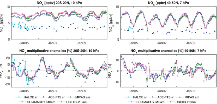
4.12.3 NO_x evaluations: Seasonal cycles ...183

4.12.4 NO_x evaluations: Interannual variability ...185

4.12.5 NO_x evaluations: Downward transport of NO_x during polar winter ...187

4.12.6 Summary and conclusions: NO_x ...187

4.13 Nitric acid – HNO₃ ... 190

4.13.1 Availability of HNO₃ measurements ...190

4.13.2 HNO₃ evaluations: Zonal mean cross sections and vertical profiles ...191

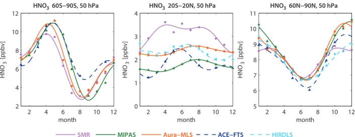
4.13.3 HNO₃ evaluations: Seasonal cycles ...194

4.13.4 HNO₃ evaluations: Interannual variability...195

4.13.5 Summary and conclusions: HNO₃ ...195

4.14 Peroxynitric acid – HNO4 ... 198

4.14.1 Availability of HNO₄ measurements ...198

4.14.2 HNO₄ evaluations: Zonal mean cross sections and vertical profiles ...199

4.14.3 Summary and conclusions: HNO₄ ...200

4.15 Dinitrogen pentoxide – N₂O₅ ... 201

4.15.1 Availability of N₂O₅ measurements ...201

4.15.2 N₂O₅ evaluations: Zonal mean cross sections and vertical profiles ...201

4.15.3 Summary and conclusions: N₂O₅ ...203

4.16 Chlorine nitrate – ClONO₂ ... 203

4.16.1 Availability of ClONO₂ measurements ...203

4.16.2 ClONO₂ evaluations: Zonal mean cross sections and vertical profiles ...204

4.16.3 Summary and conclusions: ClONO₂ ...206

4.17 Total reactive nitrogen – NOy ... 206

4.17.1 Availability of NO_y measurements ...207

4.17.2 NO_y evaluations: Zonal mean cross sections and vertical profiles ...207

4.17.3 NO_y evaluations: Seasonal cycles ...208

4.17.4 NO_y evaluations: Interannual variability ...210

4.17.5 Summary and conclusions: NO_y ...211

4.18 Hydrogen chloride – HCl ... 213

4.18.1 Availability of HCl measurements ...213

4.18.2 HCl evaluations: Zonal mean cross sections, vertical and meridional profiles ...213

4.18.3 HCl evaluations: Latitude-time evolution ...216

(2)

4.18.4 HCl evaluations: Interannual variability ...217

4.18.5 Summary and conclusions: HCl ...218

4.18.6 Recommendations: HCl ...220

4.19 Chlorine monoxide – ClO ... 220

4.19.1 Availability of ClO measurements ...220

4.19.2 ClO evaluations: Zonal mean cross sections ...221

4.19.3 ClO evaluations: Vertical and meridional profiles ...224

4.19.4 Summary and conclusions: ClO ...225

4.20 Hypochlorous acid – HOCl ... 226

4.20.1 Availability of HOCl measurements ...227

4.20.2 HOCl evaluations: Zonal mean cross sections ...228

4.20.3 HOCl evaluations: Vertical and meridional profiles ...229

4.20.4 Summary and conclusions: HOCl ...231

4.21 Bromine oxide – BrO ... 231

4.21.1 Availability of BrO measurements ...231

4.21.2 BrO evaluations: Monthly zonal mean cross sections ...232

4.21.3 BrO evaluations: Vertical and meridional profiles ...234

4.21.4 Summary and conclusions: BrO ...235

4.22 Hydroxyl radical – OH ... 236

4.22.1 Availability of OH measurements ...236

4.22.2 OH zonal mean cross sections ...237

4.22.3 OH vertical profiles from Aura-MLS ...238

4.22.4 Summary and conclusions: OH ...238

4.23 Hydroperoxy radical – HO₂ ... 239

4.23.1 Availability of HO₂ measurements ...239

4.23.2 HO₂ evaluations: Zonal mean cross sections ...239

4.23.3 HO₂ evaluations: Vertical profiles ...240

4.23.4 Summary and conclusions: HO₂ ...240

4.24 Formaldehyde – CH2O ... 242

4.24.1 Availability of CH₂O measurements ...243

4.24.2 CH₂O evaluations: Annual zonal mean cross sections ...243

4.24.3 CH₂O evaluations: Meridional profiles ...243

4.24.4 Seasonality in CH₂O ...244

4.24.5 Summary and conclusions: CH₂O ...245

4.25 Acetonitrile - CH3CN ... 246

4.25.1 Availability of CH₃CN measurements ...246

4.25.2 CH₃CN evaluations: Zonal mean cross sections ...246

4.25.3 Summary and conclusions: CH₃CN ...246

4.26 Aerosol ... 247

4.26.1 Availability of aerosol measurements ...247

4.26.2 Aerosol evaluations: Vertical and meridional profiles at similar wavelengths ...248

4.26.3 Aerosol evaluations: Altitude profiles ...253

4.26.4 Aerosol evaluations: Interannual variability...255

4.26.5 Summary and conclusions: Aerosol ...263

(3)

4.27 Upper troposphere / lower stratosphere (UTLS) ozone evaluations based on

TES averaging kernels ... 270

4.27.1 Availability of UTLS ozone satellite datasets ...271

4.27.2 TES ozone and operational operator ...271

4.27.3 UTLS ozone evaluations: Zonal mean cross sections, vertical and meridional profiles ...273

4.27.4 UTLS ozone evaluations: Seasonal cycles ...281

4.27.5 UTLS ozone evaluations: Interannual variability ...283

4.27.6 Summary and conclusions: UTLS ozone ...283

4.27.7 Recommendations: UTLS ozone ...287

Chapter 5: Implications of results ...289

5.1 Implications for model-measurement intercomparison ... 289

5.1.1 Seasonal cycles ...290

5.1.2 Vertical and meridional profiles ...295

5.1.3 Recommendations for short-lived species ...298

5.1.4 Suggestions for new diagnostics ...299

5.2 Implications for merging activities ... 301

5.2.1 Error characterisation of instruments ...301

5.2.2 Drifts and jumps between datasets ...302

5.2.3 Altitude resolution and a priori information ...303

5.3 Implications for future planning of satellite limb-sounders ... 304

References ...305

(4)

4.11 Nitrogen dioxide – NO

2

Nitrogen dioxide (NO₂) is a major air pollutant in the troposphere, and is produced mainly by fossil fuel burning (via production of NO, see Section 4.10). Natural sources of tro- pospheric NO₂ involve lightning, bacterial processes in soil and water, and biomass burning. The main source of NO₂ in the stratosphere is the oxidation of N₂O, also originat- ing from soil emissions (see Section 4.4), followed by downward transport of upper atmospheric NO_x in the winter polar vortex (up to 9%). Stratospheric NO₂ is considered an ozone depleting substance through the catalytic NO_x cycle.

At the same time, NO₂ acts as a buffer against halogen-cat- alyzed ozone loss by converting reactive chlorine, bromine, and hydrogen compounds into stable reservoir substances ( ClONO₂, BrONO₂, HNO₃). The removal of nitrogen from the stratosphere, as observed in the SH polar vortex during the formation and sedimentation of polar stratospheric clouds (PSCs), is a key microphysical process in the formation of the Antarctic polar ozone hole during spring.

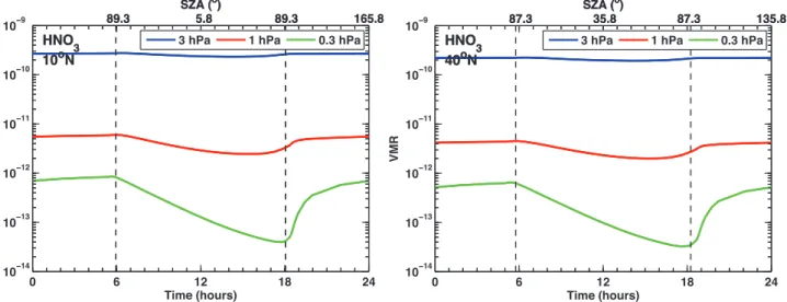
Stratospheric NO₂ variations are controlled by the sunlight- driven equilibrium between NO_x (NO, NO₂) on one hand and the reservoir substances (N₂O₅, HNO₃, ClONO₂) on the other hand. In particular, the strong diurnal NO₂ cycle complicates a comparison of satellite-based NO₂ measure- ments that correspond to different LSTs. Figure 4.11.1 shows examples of the diurnal NO₂ cycle as a function of LST for three different pressure levels as derived with a chemical box model [McLinden et al., 2010]. As seen in these plots there are large differences between day and night-time NO₂, with a steep gradient at sunrise and sunset. Solar occultation measurements are always made at SZA = 90° and can therefore be compared amongst each other. Limb scattering and emission measurements however, can correspond to different SZAs, and a direct comparison of the climatologies is not meaningful in most cases unless the dependence on the SZA is taken into account.

4.11.1 Availability of NO₂ measurements

The first vertically resolved satellite NO₂ measurements were made by LIMS in 1978/1979. SAGE II and HALOE provide the longest continuous NO₂ datasets, both ending in 2005. A number of more recent satellite missions have been measuring NO₂ from 2002 onwards. Solar occultation measurements are available from SAGE II, HALOE, POAM II, POAM III, SAGE III and ACE-FTS. Periods of maximum overlap are 1994-1996 (SAGE II, HALOE, and POAM II) and 2005 (SAGE II, HALOE, POAM III, SAGE III, and ACE-FTS). NO₂ measurements by limb emission and scattering techniques are available for OSIRIS, SCIAMACHY, and MIPAS from 2002 onward, while GOMOS provides stellar occultation measurements for the same time period.

Additionally, HIRDLS data for 2005-2007 and LIMS data for 1978-1979 exist. Table 4.11.1 summarises information on the available NO₂ measurement record including time period and vertical range.

The solar occultation climatologies can be compared directly if separated into local sunrise and local sunset measurements. Note that there is a difference between the sunrise/

sunset as seen from a satellite and the local sunrise/sunset that determines the chemical state of the measured air mass, and is therefore used to categorise the measurements.

The corresponding data files are labelled as am/pm with am LST generally corresponding to local sunrise and pm LST generally corresponding to local sunset. One deviation from the photochemical conditions at local sunrise can occur when a satellite crosses the terminator towards the polar day area at high latitudes. During such observations, the photochemical conditions of the atmosphere at local surise may be completely different than that of a typical sunrise observation because the area is continuously illuminated during polar day. The same situation can occur when the satellite crosses the terminator towards polar night. Table 4.11.2 summarises the local sunrise/sunset climatologies.

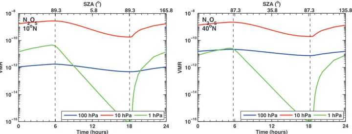
Figure 4.11.1: Diurnal NO₂ cycle. NO₂ variations as function of LST are shown at 10°N and 40°N at 1, 10 and 100 hPa for March 15.

0 6 12 18 24

10⁻¹¹ 10⁻¹⁰ 10⁻⁹ 10⁻⁸ 10⁻⁷

VMR

Time (hours)

89.3 SZA ( 5.8^o) 89.3 165.8

NO₂ 10^oN

100 hPa 10 hPa 1 hPa

0 6 12 18 24

10⁻¹¹ 10⁻¹⁰ 10⁻⁹ 10⁻⁸ 10⁻⁷

VMR

Time (hours)

87.3 SZA ( 35.8^o) 87.3 135.8

NO₂ 40^oN

100 hPa 10 hPa 1 hPa

(5)

NO₂ measurements by limb emission and scattering techniques correspond approximately to a fixed LST if the instrument has a sun-synchronous orbit (e.g., MIPAS measurements correspond to 10am and 10pm LST). The measurement LST can vary from instrument to instrument,

and may also vary for some instruments between seasons and latitudes. In order to compare other instruments (OSIRIS, SCIAMACHY, ACE-FTS) with MIPAS, their measurements have been scaled to LST 10am and 10pm with the help of a chemical box model [ McLinden et al., 2010].

Instrument Daytime climatologies Night-time climatologies

Method Corresponding LST Method Corresponding LST

LIMS Ascending orbit ~1pm Descending orbit ~11pm

OSIRIS am LST Mixed times pm LST Mixed times

Scaled 10am Scaled 10pm

SCIAMACHY No adjustments ~8am - 2pm

MIPAS am LST 10am pm LST 10pm

GOMOS No adjustments 10pm

HIRDLS SZA < 90º ~3pm SZA > 90º 00:30am

ACE-FTS Scaled 10am Scaled 10pm

Instrument Local sunrise climatologies Local sunset climatologies Satellite orbit Method Corresponding LST Method Corresponding LST

SAGE II Local sunrise am (mixed times) Local sunset pm (mixed times) non-sun-synchronous HALOE Local sunrise am (mixed times) Local sunset pm (mixed times) non-sun-synchronous POAM II Local sunrise am (mixed times) Local sunset pm (mixed times) sun-synchronous POAM III Local sunrise am (mixed times) Local sunset pm (mixed times) sun-synchronous SAGE III Local sunrise am (mixed times) Local sunset pm (mixed times) sun-synchronous ACE-FTS Local sunrise am (mixed times) Local sunset pm (mixed times) non-sun-synchronous Table 4.11.1: Available NO₂ measurement records from limb-sounding satellite instruments between 1978 and 2010.

The red filling of the grid boxes indicates the temporal and vertical coverage of the respective instrument. Instruments are grouped according to their measurement LST into the group of solar occultation instruments (upper panel) and the group of limb emission/scattering and stellar occultation instruments (lower panel).

Table 4.11.2: Overview of available NO₂ local sunrise and local sunset climatologies. For local sunrise/sunset climatolo- gies, the instrument name, the method used to derive the climatology, the corresponding LST and the satellite orbit are given.

Detailed information on the corresponding LST depending on month and latitude can be found in the data files.

Table 4.11.3: Overview of available NO₂ daytime and night-time climatologies including the 10am/pm climatologies.

For daytime and night-time climatologies, the instrument name, the method used to derive the climatology, i.e., scaling measurements or sorting measurements according to LST, orbit or SZA, and the corresponding LST range are given.

Climatologies corresponding to 10am and 10pm LST are printed in bold face. Detailed information on the corresponding LST depending on month and latitude can be found in the data files.

LIMS OSIRIS MIPAS GOMOS SCIAMACHY HIRDLS SAGE II HALOE POAM II POAM III SAGE III ACE-FTS

201020092008200720062005200420032002200120001999199819971996199519941993199219911990

1978 1979 1980 1981 1982 1983 1984 1985 1986 1987 1988 1989

(6)

For OSIRIS, scaling is done profile-by-profile, with the ini- tialisation of the model using the measured trace gas abundances and temperature. The scaling for SCIAMACHY and ACE-FTS on the other hand, is done based on lookup tables calculated from the photochemical box model initialised with climatological inputs (see Section 3.2.1). GOMOS pro- vides stellar occultation measurements at 10pm. These are evaluated with the group of limb emission and scattering instruments. The ACE-FTS climatology derived from data scaled to 10am/pm provides an opportunity to compare one solar occultation dataset with the measurements based on emission and scattering techniques. HIRDLS data from June 2005 to May 2006 have been scaled to 10am/pm with the SD-WACCM Version 3548 (SD stands for Specified Dy- namics using GEOS5.1) [Garcia et al., 2007]. Table 4.11.3 summarises all available daytime and night-time NO₂ climatologies including the original available daytime and night-time climatologies and the ones scaled to 10am/pm LST. All instruments listed in Table 4.11.3, except for ACE- FTS, are in sun-synchronous orbits. Table 4.11.4 compiles information on all NO₂ measurements, including time period, vertical range and resolution, and references relevant for the data product used in this report.

4.11.2 NO₂ evaluations: Zonal monthly mean cross sections and vertical profiles of local sunrise/sunset climatologies Local sunrise NO₂ climatologies from the solar occultation

instruments SAGE II, HALOE, ACE-FTS, SAGE III, POAM II, and POAM III are displayed in Figure 4.11.2.

The annual zonal mean climatologies are calculated over the respective lifetime of each instrument. In general, the zonal mean distribution shows the largest NO₂ abundances around 10 hPa, with maximum values at high latitudes. The three solar occultation instruments in a non-sun-synchronous orbit (SAGE II, HALOE, ACE-FTS) offer near-global coverage over the course of a year, while the three instruments in a sun-synchronous orbit (SAGE III, POAM II, and POAM III) provide measurements in a narrow range at high latitudes. The higher annual mean abundances report- ed by the first group of instruments when compared to the latter may be the result of varying seasonal coverage instead of an actual measurement bias. One example of the compli- cations arising from the varying data coverage is the evaluation of 1994-1996 POAM II local sunrise monthly zonal means that show no direct overlap with any of the other datasets. (Note that the overlap of the annual means vis- ible in Figure 4.11.2 does not necessarily correspond to an overlap of the monthly zonal means.) Moreover, the instruments with near-global coverage over the course of a year or season (SAGE II, HALOE and ACE-FTS) have strongly varying data coverage from month to month. Therefore, the comparison of annual zonal means, as carried out for the long-lived trace gases, may not be meaningful, and instead a comparison of monthly zonal means will be presented.

Note that the data coverage problem is intensified by the necessary separation into local sunrise and sunset data.

Instrument Time period Vertical range Vertical

resolution References Additional comments LIMS V6.0 Nov 78 – May 79 Cloud top – 50 km

(+ mesosphere for polar night)

3.7 km Remsberg et al., 2010

SAGE II V6.2 Oct 84 – Aug 05 Cloud top – 50 km 1.0 km (< 38 km)

5.0 km (> 38 km) Cunnold et al., 1991 Only satellite SS data are used HALOE V19 Oct 91 – Nov 05 up to 50 km 2.5 km Grooß and Russell,

2005

POAM II V6.0 Oct 93 – Nov 96 20 – 40 km 1.5 – 2.5 km Lumpe et al., 1997 Randall et al., 1998 POAM III V4.0 Apr 98 – Dec 05 20 – 40 km 1.5 – 2.5 km Lumpe et al., 1997 Randall et al., 1998 OSIRIS V3-0 Oct 01 – 13 – 45 km 2 km Brohede et al., 2007a

Brohede et al., 2007b

SAGE III V4.0 May 02 – Dec 05 Cloud top – 50 km 0.5 ~ 1.0 km Only solar occultation products used MIPAS

V15

V220 Mar 02 – Mar 04

Jan 05 – Apr 12 12 – 50/70 km

(day/night) 3 – 6 km

2.5 – 6 km Funke et al., 2005a

Funke et al., 2005b Change in spectral resolution in 2005 GOMOS V5.0 Mar 02 – Apr 12 20 – 50/70 km 4 km Kyrölä et al., 2010a

SCIAMACHY

V3-1 Sep 02 – Apr 12 11 – 42 km 3 – 5 km Bauer et al., 2012 ACE-FTS V2.2 Mar 04 – 7 – 52 km 3 – 4 km Kerzenmacher et al.,

2008

HIRDLS V6.0 Jan 05 – Jan 08 20 – 50 km 1 km Gille and Gray, 2011

Table 4.11.4: Time period, vertical range, vertical resolution, references and other comments for NO₂ measurements.

(7)

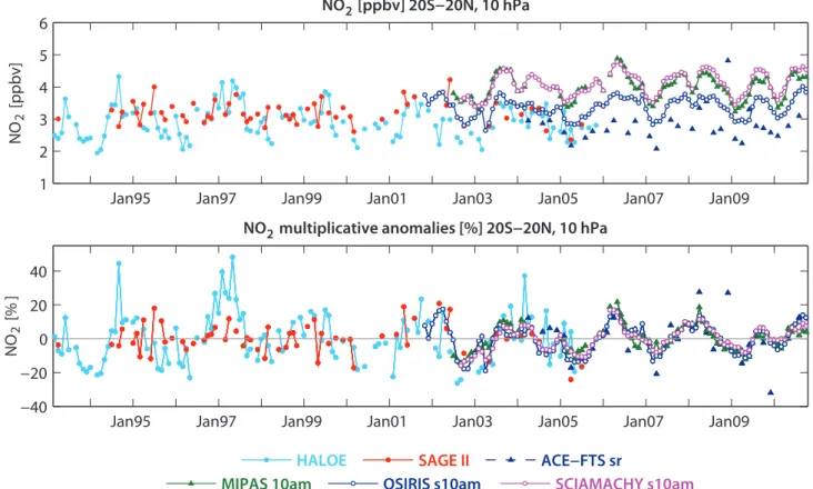
As a first step, the evaluations of local sunrise and sunset climatologies will focus on the comparison of the two longer time series from SAGE II and HALOE during their overlap time period 1992-2005. The other instruments will be compared to SAGE II and HALOE for time periods that allow as many instruments as possible to be included (1994-1996 for POAM II, 2004-2005 for ACE-FTS, POAM III, SAGE III).

SAGE II and HALOE (1992-2005)

Figure 4.11.3 shows NO₂ local sunrise and sunset monthly mean climatologies for SAGE II and HALOE for April and October. The monthly multi-annual means of the two datasets overlap in both hemispheres. The sunset climatologies show notably more NO₂ than the sunrise climatologies as a result of N₂O₅ photolysis, which is driven by the available

50S 0 50N

0.1

1

10

100

Pressure [hPa]

NO₂ HALOE Apr 92−05

50S 0 50N

0.1

1

10

100

Pressure [hPa]

NO₂ SAGE II Apr 92−05

Latitude

50S 0 50N

NO₂ HALOE Oct 92−05

50S 0 50N

NO₂ SAGE II Oct 92−05

Latitude

50S 0 50N

ppbv

0 0.4 0.8 12 4 6 8

50S 0 50N

Latitude NO₂ SAGE II Apr 92−05

50S 0 50N

Latitude

Figure 4.11.3: Cross sections of monthly zonal mean, local sunrise and sunset NO₂ for 1992-2005. Monthly zonal mean, local sunrise (column 1 and 2) and local sunset (column 3 and 4) NO₂ cross sections for April and October are shown for HALOE (upper row) and SAGE II (lower row).

50S 0 50N

NO₂ HALOE (92−05)

50S 0 50N

NO₂ ACE−FTS (04−10)

50S 0 50N

0.1

1

10

100

Pressure [hPa]

NO₂ SAGE II (85−05)

0 0.4 0.8 1 2 4 6 8

50S 0 50N

0.1

1

10

100

Pressure [hPa]

Latitude NO₂ SAGE III (02−05)

ppbv

50S 0 50N

NO₂ POAM II (94−96)

Latitude

50S 0 50N

NO₂ POAM III (98−05)

Latitude

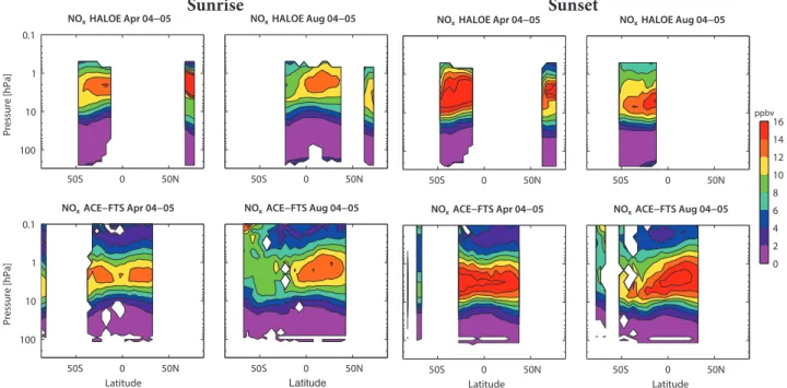
Figure 4.11.2: Cross sections of annual zonal mean, local sunrise NO₂ for solar occultation instruments. Annual zonal mean, local sunrise NO₂ cross sections are shown for the SAGE II (1985-2005), HALOE (1992-2005), ACE-FTS (2004-2010), SAGE III (2002-2005), POAM II (1994-1996), and POAM III (1998-2005).

Sunrise Sunset

(8)

sunlight and reactivates NO₂ from its reservoir species.

The N₂O₅ photolysis during daytime is fast enough that by sunset nearly all N₂O₅ is converted to NO₂, leading to a nearly symmetric distribution at the equator independent of the time of year. The N₂O₅ production during night- time is somewhat slower, and as a result larger NO₂ sunrise abundances are observed for shorter nights (e.g., in the SH during October).

The relative differences of SAGE II and HALOE from their MIM in April and October are displayed in Figure 4.11.4.

At the level of maximum NO₂ abundance (10 hPa), the two datasets agree well with differences from the MIM of up to ±10% (corresponding to differences of 20% between the two instruments). Above and below this level, the

relative differences increase steadily reaching values of up to ±50% at 2 hPa and 20/50 hPa for local sunset/sunrise climatologies. The steadily increasing differences below and above the maximum are related to the smaller vertical gradients in SAGE II NO₂ compared to HALOE. At around 10 hPa, HALOE detects more NO₂ than SAGE II, but above and below the maximum it quickly reaches lower values due to its stronger gradients and shows mostly negative differences when compared to SAGE II. Exceptions to this pattern are the local sunrise climatologies in the summer (Figure A4.11.2 in Appendix A4) and autumn hemispheres (Figure 4.11.4) when HALOE shows positive differences from the MIM everywhere below 2 hPa. Overall, the NO₂ local sunrise and sunset evaluations give a consistent picture, however, some small differences exist (e.g., sunset differences

0 5 10

0.1

1

10

100

Pressure [hPa]

50N − 55N, Jun (94−96)

NO₂ [ppbv]

HALOE SAGE II POAM II MIM

0 5 10

60S − 65S, Dec (94−96)

NO₂ [ppbv]

−40 −20 0 20 40 50N − 55N, Jun (94−96)

rel diff from MIM [%]

−40 −20 0 20 40 60S − 65S, Dec (94−96)

Figure 4.11.5: Profiles of zonal mean, local sunset NO₂ for 1994-1996. Zonal mean, local sunset NO₂ profiles for 50ºN- 55ºN for June and 60ºS-65ºS for December are shown with their differences from the MIM. Bars indicate the uncertainties in each climatological mean based on the SEM. The grey shaded area indicates where relative differences are smaller than ±5%.

50S 0 50N

0.1

1

10

100

Pressure [hPa]

NO₂ HALOE − MIM Apr 92−05

50S 0 50N

0.1

1

10

100

Pressure [hPa]

NO₂ SAGE II − MIM Apr 92−05

Latitude

50S 0 50N

NO₂ HALOE − MIM Oct 92−05

50S 0 50N

NO₂ SAGE II − MIM Oct 92−05

Latitude

50S 0 50N

%

−100

−50

−20

−10

−5

−2.5 0 2.5 5 10 20 50 100

50S 0 50N

Latitude NO₂ SAGE II − MIM Apr 92−05

50S 0 50N

NO₂ SAGE II − MIM Oct 92−05

Latitude

Figure 4.11.4: Cross sections of monthly zonal mean, local sunrise and sunset NO₂ differences for 1992-2005. Monthly zonal mean, local sunrise (column 1 and 2) and local sunset (column 3 and 4) NO₂ differences for April, and October between the individual instruments (SAGE II, HALOE) and their MIM are shown.

(9)

show a stronger hemispheric symmetry consistent with the same feature observed for the sunset mixing ratios).

SAGE II, HALOE, and POAM II (1994-1996)

As a consequence of the gaps in temporal and spatial coverage of POAM II, a direct comparison of local sunrise NO₂ climatologies from POAM II and the other two instruments is not possible. However, for NO₂ sunset measurements, some months and latitude bands exist where all three datasets overlap, allowing for a direct comparison of POAM II, SAGE II and HALOE. Vertical profiles from all three instrument local sunset climatologies and their relative differences from the MIM are displayed in Figure 4.11.5.

In both latitude bands (NH and SH mid-latitudes), the POAM II climatology reports smaller values than SAGE II and HALOE, with differences with respect to the MIM of -10%. Above 7 hPa, POAM II agrees better with HALOE than with SAGE II, while below 7 hPa the situation is reversed.

SAGE II, HALOE, POAM III, SAGE III, and ACE-FTS (2004-2005) For the period 2004-2005, the long NO₂ time series from SAGE II and HALOE overlap with the more recent data from

ACE-FTS. Also available during this period are datasets from SAGE III and POAM III, which focus on narrow latitude rang- es. A comparison of SAGE III and POAM III zonal monthly mean cross sections is not possible, therefore the evaluation of these two climatologies will be based on vertical profiles.

Figure 4.11.6 shows NO2 local sunrise and sunset monthly mean climatologies for SAGE II, HALOE, and ACE-FTS for April and October. Note that SAGE II and HALOE have less latitudinal coverage for 2004-2005 (the last two years of their lifetimes) when compared to earlier time periods (e.g., Figure 4.11.3). The respective relative differences between the individual datasets and their MIM are presented in Figure 4.11.7. Overall, the magnitude and spread of the relative differences are similar to those already discussed for the long-term comparison of SAGE II and HALOE, with the smallest differences (up to ±10%) around 10 hPa, and larger differences (up to ±50%) above 2 hPa and below 50 hPa. Note that for some cases the differences are below ±20% for the complete altitude range from 1 to 100 hPa (e.g., sunset differences of SAGE II and ACE-FTS to their MIM for SH October). For the local sunrise climatologies, ACE-FTS shows the largest, and HALOE the lowest NO₂ abundances. For the local sunset climatologies, SAGE II show the largest and HALOE the lowest NO₂ abundances, with ACE-FTS values between the other two

50S 0 50N

0.1

1

10

100

Pressure [hPa]

50S 0 50N

0.1

1

10

100

Pressure [hPa]

NO₂ SAGE II Apr 04−05

50S 0 50N

0.1

1

10

100

Pressure [hPa]

NO₂ ACE−FTS Apr 04−05

Latitude

50S 0 50N

NO₂ ACE−FTS Oct 04−05

Latitude

50S 0 50N

NO2 HALOE Apr 04−05

50S 0 50N

NO2 SAGE II Apr 04−05 ^ppbv

0 0.4 0.81 2 4 6 8

50S 0 50N

NO2 ACE−FTS Apr 04−05

Latitude

50S 0 50N

NO2 HALOE Oct 04−05

50S 0 50N

NO2 SAGE II Oct 04−05

50S 0 50N

NO2 ACE−FTS Oct 04−05

Latitude

Figure 4.11.6: Cross sections of monthly zonal mean, local sunrise and sunset NO₂ for 2004-2005. Monthly zonal mean, local sunrise (column 1 and 2) and local sunset (column 3 and 4) NO₂ cross sections for April and October are shown for the HALOE, SAGE II, and ACE-FTS.

(10)

instruments. The only exception is found at 10 hPa where HALOE detects a larger NO₂ peak than the other two datasets, consistent with the evaluations of the earlier time period. Overall, ACE-FTS agrees better with SAGE II than with HALOE.

A comparison of POAM III and SAGE III with the other data- sets is shown in Figure 4.11.8 as vertical profiles and their relative differences from the MIM. The months and latitude bands used for this comparison are chosen because the coverage includes the maximum number of datasets available.

The profiles confirm the good agreement of all instruments

50S 0 50N

0.1

1

10

100

Pressure [hPa]

50S 0 50N

0.1

1

10

100

Pressure [hPa]

NO₂ SAGE II − MIM Apr 04−05

50S 0 50N

0.1

1

10

100

Pressure [hPa]

NO2 ACE−FTS − MIM Apr 04−05

Latitude

50S 0 50N

NO2 ACE−FTS − MIM Oct 04−05

Latitude

50S 0 50N

NO₂ SAGE II − MIM Apr 04−05

−100

−50

−20

−10

−5

−2.5 0 2.5 5 10 20 50 100

0 0.5 1

Latitude

NO₂ ACE−FTS − MIM Apr 04−05

50S 0 50N

NO₂ ACE−FTS − MIM Oct 04−05

Latitude

%

Figure 4.11.7: Cross sections of monthly zonal mean, local sunrise and sunset NO₂ differences for 2004-2005. Monthly zonal mean, local sunrise (column 1 and 2) and local sunset (column 3 and 4) NO₂ differences for April and October between the individual instruments (HALOE, SAGE II, ACE-FTS) and their MIM are shown.

Figure 4.11.8: Profiles of zonal mean, local sunset NO₂ for 2004-2005. Zonal mean, local sunset NO₂ profiles for 65ºN-70ºN for March and 60ºN-65ºN for April are shown together with their differences from the MIM. Bars indicate the uncertainties in each climatological mean based on the SEM. The grey shaded area indicates where relative differences are smaller than ±5%.

0 2 4 6 8

0.1

1

10

100

Pressure [hPa]

65N − 70N, Mar (04−05)

NO₂ [ppbv]

0 2 4 6 8

60N − 65N, Apr (04−05)

NO₂ [ppbv]

−40 −20 0 20 40 65N − 70N, Mar (04−05)

−40 −20 0 20 40 60N − 65N, Apr (04−05)

HALOE ACE-FTS SAGE II SAGE III POAM III MIM

(11)

in the MS with differences often below ±5%, except for a divergence between ACE-FTS and SAGE III in March which show differences from the MIM of up to ±10%. Dif- ferences are large in the LS and USLM consistent with low NO₂ abundances. However, there is a much better agreement between 50 and 10 hPa (below the NO₂ VMR peak) compared to between 5 and 1 hPa (above the NO₂ peak) for similar NO₂ background abundances. In general, SAGE III is similar to SAGE II and shows larger NO₂ values than the other datasets, while POAM III values reside mostly in the middle.

4.11.3 NO₂ evaluations: Zonal monthly mean cross sections of 10am/pm climatologies

NO₂ measurements by limb emission and scattering techniques and from stellar occultation have been sorted according to LST or scaled with the help of chemical box models (see Section 4.11.1 for details). Additionally, the solar occultation dataset from ACE-FTS has been scaled to allow for a first-step comparison between the two groups of instruments. In the following, climatologies corresponding to 10am and 10pm will be compared with each other.

For a better understanding of the scaling effects, the ini- tial climatologies are also shown. Note that the 10am/pm

climatologies are part of the larger groups of daytime/

night-time climatologies as explained in Table 4.11.3.

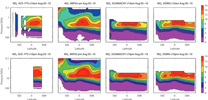
OSIRIS, SCIAMACHY, MIPAS, GOMOS, HIRDLS, and ACE-FTS (2005-2007)

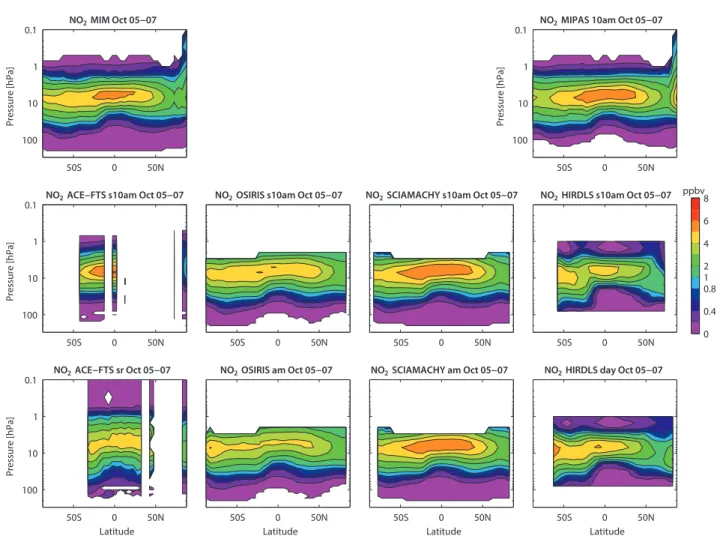
Figure 4.11.9 shows the NO2 10am climatologies for October 2005-2007 that can be directly compared to each other: MIPAS (corresponding to 10am LST) and ACE-FTS, OSIRIS, SCIAMACHY, and HIRDLS, all scaled to 10am LST (labelled as s10am in the figure titles). Additionally, unscaled daytime data from SCIAMACHY and OSIRIS (corresponding to a range of LSTs), HIRDLS daytime measurements (corresponding to 3pm), and ACE-FTS local sunrise measurements are shown. The overall NO₂ distribution shows flat isopleths and maximum abundances in the subtropics between 5 and 10 hPa. Note that the elevated values observed by MIPAS at very high NH latitudes are related to small changes of the LST from 10am and the timing of sunsets/sunrises (near 10am) during October. Similarly, MIPAS shows elevated values at high SH latitudes for April (see Figure A4.11.6 in Appendix A4).

The MIM is calculated based on MIPAS and scaled ACE- FTS, OSIRIS, SCIAMACHY, and HIRDLS climatologies

50S 0 50N

0.1

1

10

100

NO₂ MIM Oct 05−07

Pressure [hPa]

50S 0 50N

0.1

1

10

100

Latitude

Pressure [hPa]

NO₂ ACE−FTS sr Oct 05−07

50S 0 50N

0.1

1

10

100

Pressure [hPa]

NO₂ ACE−FTS s10am Oct 05−07

0 0.4 0.81 2 4 6 8

50S 0 50N

0.1

1

10

100

NO₂ MIPAS 10am Oct 05−07

Pressure [hPa]

50S 0 50N

NO₂ OSIRIS s10am Oct 05−07

50S 0 50N

NO₂ SCIAMACHY s10am Oct 05−07

50S 0 50N

NO₂ HIRDLS s10am Oct 05−07

50S 0 50N

NO₂ OSIRIS am Oct 05−07

Latitude

50S 0 50N

NO₂ SCIAMACHY am Oct 05−07

Latitude

50S 0 50N

NO₂ HIRDLS day Oct 05−07

Latitude

ppbv

Figure 4.11.9: Cross sections of zonal mean daytime NO₂ for October 2005-2007. Monthly zonal mean NO₂ cross sections for October 2005-2007 are shown for the MIM (upper left panel) and the individual instruments. Measurements correspond to 10am LST (MIPAS) or are scaled to 10am LST. Note that scaled HIRDLS data are only available for June 2005 – May 2006. In addition, unscaled data from ACE-FTS, OSIRIS, SCIAMACHY, and HIRDLS are shown.

(12)

for 2005-2007. Differences of the individual datasets from the MIM for October 2005-2007 are shown in Figure 4.11.10. In general, the differences in the MS vary strongly, from ±5% in some regions to ±50% in others. MIPAS and SCIAMACHY show similar features and observe larger NO₂ abundances than the other instruments, leading to deviations from the MIM in the MS of around +20%, and locally +50%. One exception is the SH extra-tropics where both instruments show negative differences from the MIM of up to -20%. While MIPAS and SCIAMACHY are on the high side, HIRDLS observes values at the lower end of the range, producing large negative deviations from the MIM of up to -50% (and locally -100%). An exception to this be- haviour is again the SH extra-tropics where HIRDLS detects larger NO₂ abundances than the other instruments.

OSIRIS is mostly in the middle range; deviations from the MIM change sign depending on the latitude band and ex- ceed ±50% only occasionally. ACE-FTS also observes deviations of mixed signs, mostly opposite to HIRDLS with particularly large negative deviations where HIRDLS shows a positive difference. Note that at high SH latitudes, where only MIPAS, OSIRIS and SCIAMACHY measurements are available, the three instruments agree considerably better, with deviations from their MIM of only up to ±20%, while in regions where all five instruments provide measurements, deviations can reach ±50% to ±100%. Evaluations of

January, April, and July climatologies (see Figure A4.11.6 in Appendix A4 for April evaluations) give a consistent picture for all four seasons. The main difference from the October evaluations discussed above is that MIPAS and HIRDLS show more differences of mixed signs. While in the SH spring and summer, MIPAS is mostly positive and HIRDLS mostly negative, MIPAS deviations from the MIM in the NH spring and summer are negative almost everywhere below 10 hPa. The pattern of OSIRIS deviations from the MIM changes from month to month. Note that scaled HIRDLS data are only available for June 2005 – May 2006, and that the evaluation of this one-year long time period (not shown) gives very similar results to the evaluation presented above.

For a better understanding of the scaling effects, the ini- tial climatologies are also shown. The unscaled OSIRIS and ACE-FTS datasets have a considerably larger bias compared to the scaled datasets, indicating that scaling is necessary in order to compare the climatologies. SCIAMACHY shows similar differences for the scaled and unscaled datasets, which can be explained by the fact that the LST of the original SCIAMACHY dataset is 10am at the equator and only changes slightly when moving to higher latitudes. For some regions (e.g., SH in March) the scaled dataset shows somewhat larger differences from the MIM than the unscaled

50S 0 50N

0.1

1

10

100

NO₂ ACE−FTS sr Oct 05−07

Pressure [hPa]

Latitude

50S 0 50N

0.1

1

10

100

NO₂ ACE−FTS s10am Oct 05−07

Pressure [hPa]

50S 0 50N

0.1

1

10

100

Pressure [hPa]

NO2 MIPAS 10am Oct 05−07

50S 0 50N

NO₂ OSIRIS s10am Oct 05−07

50S 0 50N

NO₂ SCIAMACHY s10am Oct 05−07

50S 0 50N

NO₂ HIRDLS s10am Oct 05−07

−100−50

−20

−10−5

−2.50 2.55 1020 50100

50S 0 50N

NO₂ OSIRIS am Oct 05−07

Latitude

50S 0 50N

NO₂ SCIAMACHY am Oct 05−07

Latitude

50S 0 50N

Latitude NO₂ HIRDLS day Oct 05−07

%

Figure 4.11.10: Cross sections of zonal mean daytime NO₂ differences for October 2005-2007. Monthly zonal mean NO₂ differences from the MIM for October 2005-2007 are shown. Measurements correspond to 10am LST (MIPAS) or are scaled to 10am LST. Note that scaled HIRDLS data are only available for June 2005 – May 2006. In addition, unscaled data from ACE- FTS, OSIRIS, SCIAMACHY, and HIRDLS are shown.

(13)

dataset, unlike the results from OSIRIS. In these cases, it is possible that the errors introduced by the scaling based on look up tables outweigh the improvement achieved by the correction to a specific LST. For HIRDLS, large negative deviations are apparent in the scaled and unscaled datasets, indicating that the differences are related to measurement differences and cannot be corrected by accounting for the measurement LST.

NO₂ night-time climatologies for October 2005-2007 are shown in Figure 4.11.11. NO₂ abundances are considerably larger for the night-time climatologies than for daytime climatologies, as expected from the diurnal cycle. Maximum NO₂ values can be observed in the SH mid-latitudes and tropics between 1 and 10 hPa. As for the daytime climatologies, MIPAS data (corresponding to 10pm LST) as well as scaled ACE-FTS, OSIRIS, SCIAMACHY and HIRDLS data (all scaled to 10pm LST) are available and can be compared directly. Additionally, GOMOS measures night-time NO₂ at 10pm LST. Also shown in Figure 4.11.11 are the unscaled OSIRIS night-time climatology (corresponding to a range of LSTs), the HIRDLS night-time climatology (corresponding to approximately 00:30am) and the ACE- FTS local sunset climatology. Note that for SCIAMACHY no measurements during the night exist and that the scaled

10pm SCIAMACHY climatology is based on daytime SCIAMACHY measurements.

Differences of the individual night-time climatologies from the MIM are displayed in Figure 4.11.12. The MIM is based on the climatologies corresponding directly to 10pm LST (MIPAS, GOMOS), and scaled to 10pm LST (ACE- FTS, OSIRIS, SCIAMACHY and HIRDLS). MIPAS and SCIAMACHY have positive deviations in the MS and negative deviations in the LS, and agree well with each other and with OSIRIS. The climatologies from HIRDLS and ACE- FTS show lower values for most latitude bands, with deviations from the MIM of up to -50%. The GOMOS dataset is somewhat noisier than the other climatologies but shows small differences from the MIM (up to ±10%) between 10 and 1 hPa. In the LS, MIPAS, SCIAMACHY and ACE-FTS observe the lowest values while GOMOS and OSIRIS show positive deviations from the MIM. Differences can become as large as ±100% locally. Note that SCIAMACHY data scaled to 10pm represent a scaling to completely different illumination conditions, namely from day to night, while the scaling of SCIAMACHY data to 10am is a daytime to daytime scaling, with only slightly different illumination conditions. The fact that the SCIAMACHY night-time climatology does not show larger differences from the MIM

50S 0 50N

0.1

1

10

100

NO₂ MIM Oct 05−07

Pressure [hPa]

50S 0 50N

0.1

1

10

100

Latitude

Pressure [hPa]

NO₂ ACE−FTS ss Oct 05−07

50S 0 50N

0.1

1

10

100

Pressure [hPa]

NO₂ ACE−FTS s10pm Oct 05−07

0 0.4 0.81 2 4 6 8 10

50S 0 50N

NO₂ MIPAS 10pm Oct 05−07

50S 0 50N

NO₂ OSIRIS s10pm Oct 05−07

50S 0 50N

NO₂ SCIAMACHY s10pm Oct 05−07

50S 0 50N

NO₂ GOMOS 10pm Oct 05−07

50S 0 50N

NO₂ HIRDLS s10pm Oct 05−07

50S 0 50N

NO₂ OSIRIS pm Oct 05−07

Latitude

50S 0 50N

NO₂ HIRDLS night Oct 05−07

Latitude

ppbv

Figure 4.11.11: Cross sections of zonal mean night-time NO₂ for October 2005-2007. Monthly zonal mean NO₂ cross sections for October 2005-2007 are shown for the MIM (upper panel) and the individual instruments. Measurements correspond to 10pm LST (MIPAS, and GOMOS) or are scaled to 10pm LST. Note that scaled HIRDLS data are only available for June 2005 – May 2006. In addition, unscaled data from ACE-FTS, OSIRIS, and HIRDLS are shown.

(14)

than the daytime climatology suggests that no large errors have been introduced by this scaling procedure.

A comparison of the night-time climatologies without GOMOS (see Figure A4.11.9 in Appendix A4) shows that the observed differences are quite similar to the daytime evaluations, and that both sets of climatologies provide a consistent picture. Note that differences are slightly smaller between the night-time climatologies than between the daytime climatologies, which might be related to the larger NO₂ abundances during night-time.

In addition to the NO₂ datasets discussed above, which cover the time period after 2000, the very first satellite borne NO₂ profile measurements from the limb emission instrument LIMS are available for 1978/1979. The LIMS daytime climatology corresponds to 1pm at low and mid- latitudes and shifts to late afternoon at higher latitudes, while the LIMS night-time climatology corresponds approximately to 11pm LST. Since there are no daytime or night-time NO₂ measurements available before 2002, LIMS will be compared to the 2005-2007 climatologies presented above. Note that the stratospheric aerosol content is very low for both time periods, which facilitates the comparison of LIMS NO₂ with the other datasets.

Figure 4.11.13 shows the relative differences of LIMS day- and night-time climatologies to the respective 10am/pm 2005-2007 MIM from the evaluations above. LIMS shows good agreement in a narrow pressure range between 10 and 5 hPa, with differences mostly between ±10%. Below this level differences increase quickly, reaching +100% in the LS. Above this level, the daytime climatologies differ by up to -50% while the night-time climatologies show slightly better agreement, with differences of up to -20%. Note that LIMS measurements are not taken at 10am or 10pm LST, and it is therefore not possible to easily separate the differences attributable to a real measurement bias, and the effects of the diurnal NO₂ cycle.

4.11.4 NO₂ evaluations: Seasonal cycles

NO₂ exhibits a strong seasonal cycle in the extra-tropics due to the effects of sunlight on the partitioning of the NO_y family. Seasonal cycles of the NO₂ daytime and night-time climatologies will be evaluated below. Since the seasonal variations of the sunset and sunrise climatologies from the solar occultation instruments can be difficult to analyse due to sparse data coverage, they are not shown here.

50S 0 50N

0.1

1

10

100

NO₂ ACE−FTS ss Oct 05−07

Pressure [hPa]

Latitude

50S 0 50N

0.1

1

10

100

NO₂ ACE−FTS s10pm Oct 05−07

Pressure [hPa]

50S 0 50N

NO₂ MIPAS 10pm Oct 05−07

50S 0 50N

NO₂ OSIRIS s10pm Oct 05−07

50S 0 50N

NO₂ SCIAMACHY s10pm Oct 05−07

−100

−50−20

−10−5

−2.50 2.5 510 2050 100

50S 0 50N

0.1

1

10

100

Pressure [hPa]

NO₂ GOMOS 10pm Oct 05−07

50S 0 50N

NO₂ HIRDLS s10pm Oct 05−07

50S 0 50N

NO₂ OSIRIS pm Oct 05−07

Latitude

50S 0 50N

Latitude NO₂ HIRDLS night Oct 05−07

%

Figure 4.11.12: Cross sections of zonal mean night-time NO₂ differences for October 2005-2007. Monthly zonal mean NO₂ differences from the MIM for October 2005-2007 are shown. Measurements correspond to 10pm LST (MIPAS, and GOMOS) or are scaled to 10pm LST. Note that scaled HIRDLS data are only available for June 2005 – May 2006. In addition, unscaled data from ACE-FTS, OSIRIS, and HIRDLS are shown.