Peruvian Oxygen Minimum Zone for the last 22,000 years and the benthic foraminiferal response to (de)oxygenation
Dissertation
Submitted for the degree of Doctorate in Natural Sciences
Dr. rer. nat. der
zur Erlangung des Doktorgrades Dr. rer. nat. der
Faculty of Mathematics and Nature Science Christian-Albrechts-University of Kiel Mathematisch Naturwissenschaftlichen Fakultät
der ChristianAlbrechts Universität zu Kiel
submitted by
vorgelegt von
Zeynep Erdem
Kiel, May 2016
Erster Gutachter: Prof. Dr. Wolf-Christian Dullo Zweiter Gutachter: Prof. Dr. Dirk Nürnberg Tag der Disputation: 16.06.2016
Zum Druck genehmigt:
Declaration
I, Zeynep Erdem, hereby declare that apart from the guidance of my supervisors, I have independently and entirely conducted this doctoral work and written the dissertation without any kind of unauthorized aid. Neither this nor a similar work has been published, submitted for publication, or submitted for an examination procedure to another department or institution. I assure that the presented research project has been conducted in full compliance with the rules of good scientific practice laid by the German Research Foundation (DFG).
Kiel, ... ...………
Zeynep Erdem, M.Sc.
Erklärung
Hiermit erkläre ich, Zeynep Erdem, dass ich, abgesehen von der Unterstützung meiner Betreuer, diese Doktorarbeit eigenständig und ohne unerlaubte Hilfe durchgeführt habe. Weder diese noch eine ähnliche Arbeit wurde an einer anderen Abteilung oder Hochschule im Rahmen eines Prüfungsverfahrens vorgelegt, veröffentlicht oder zur Veröffentlichung vorgelegt. Ich versichere, dass die Arbeit unter Einhaltung der guten wissenschaftlichen Praxis der Deutschen Forschungsgemeinschaft entstanden ist.
Kiel, ... ...………
Zeynep Erdem, M.Sc.
i
Zusammenfassung ... vi
Abbreviations ... ix
1. INTRODUCTION ... 1
1.1. Motivation and previous work ... 1
1.2. Outline ... 3
1.3. Declaration of contribution ... 4
1.4. Study Area ... 5
1.4.1. Present Hydrodynamics of the Eastern Equatorial Pacific ... 5
1.4.2. The Peruvian OMZ & Upwelling ... 8
1.4.3. Sediment distribution along the Peruvian margin ... 10
1.5. Micropaleontological proxies: benthic foraminifera ... 11
1.5.1. Benthic foraminifera in oxygen depleted habitats ... 12
1.5.2. Benthic foraminifera of the Eastern Equatorial Pacific OMZs ... 15
2. METHODOLOGY AND STRATIGRAPHIES OF THE SEDIMENT CORES... 17
2.1. Age models of the sediment cores ... 19
2.2. Core specific information ... 22
3. PERUVIAN SEDIMENTS AS RECORDERS OF AN EVOLVING HIATUS FOR THE LAST 22 THOUSAND YEARS ... 33
3.1. Introduction ... 35
3.2. Regional setting ... 35
3.2.1. Physical Oceanography ... 36
3.2.2. Sediments and topography of Peruvian margin ... 39
3.3. Material and Methods ... 40
3.3.1. Chronostratigraphy ... 40
3.3.2. Determination of critical slope areas ... 43
3.4. Results ... 45
3.4.1. General facies distribution ... 45
3.4.2.Sediments of the time windows: Recent, late and early Holocene, BA, HS1 and LGM ... 46
3.4.3. Distribution of phosphorites ... 48
3.4.4. Near critical slope areas ... 49
3.5. Discussion ... 50
3.5.1. Phosphorites as erosion indicators ... 52
ii
3.5.3. Potential effects of mid-depth hydrodynamic change ... 55
3.6. Conclusions ... 56
4. DOWNCORE BENTHIC FORAMINIFERAL DISTRIBUTIONS FROM THE PERUVIAN MARGIN FOR THE LAST 22,000 YEARS... 59
4.1. General trends... 59
4.2. The most abundant species and their indications ... 68
5. BOTTOM-WATER DEOXYGENATION AT THE PERUVIAN MARGIN DURING THE LAST DEGLACIATION RECORDED BY BENTHIC FORAMINIFERA ... 71
5.1. Introduction ... 72
5.1.1. Benthic foraminifera as oxygen proxy ... 74
5.1.2. Regional setting... 77
5.2. Materials and Methods ... 78
5.2.1. Sediment cores ... 78
5.2.2. Surface samples and living benthic foraminifera ... 78
5.2.3. Statistical analyses ... 82
5.3. Results and Discussion ... 83
5.3.1. Living benthic foraminiferal distributions ... 83
5.3.2. Results and interpretation of statistical analyses... 85
5.3.3. Quantification of BWO concentrations: downcore records ... 89
5.3.4. Comparison with other proxies and records from the EEP ... 94
5.4. Summary and Conclusions ... 97
6. SUMMARY AND OUTLOOK ... 99
6.1. Summary ... 99
6.2. Outlook ... 102
REFERENCES... 105
APPENDIX ... 123
Thank you ... 195
Curriculum Vitae... 197
iii
The Eastern Equatorial Pacific (EEP) is characterized by oxygen depleted waters as result of intense upwelling, enhanced surface primary productivity and sluggish ventilation of the subsurface waters. The dynamics of these oxygen minimum zones (OMZs) are closely related to changing climatic conditions with recent observations indicating these zones are expanding as the atmosphere and oceans warm. To advance our understanding of the OMZs and improve modelling under future warming, we need to decipher the dynamics of dissolved oxygen during past periods of temperature fluctuation, such as during glacial-interglacial transitional periods.
The Peruvian margin hosts one of the strongest OMZs in the todays’ oceans and has long been in the focus of (paleo)-oceanographic investigations. Many paleo-proxy records from the region indicate increased oxygen depletion during the last deglaciation, Termination I. This present study investigated the potential changes in the structure and shape of the OMZ since the Last Glacial Maximum (LGM) using downcore distributions of the benthic foraminiferal assemblages. The sediment cores considered in this study were recovered from the lower oxic- suboxic boundary of the OMZ in order to reconstruct temporal and spatial changes in the extension of the OMZ. Using benthic foraminifera to quantify past bottom-water oxygen concentrations was a particular focus of this study. In addition to oxygen reconstruction, this study focused on the erosional features and gaps found in the sediment records in order to investigate the potential changes in the mid-depth hydrodynamics since the LGM. Variations within the subsurface and intermediate waters might lead changes in the ventilation of bottom- waters, thus the oxygenation.
Chronostratigraphies of nine sediment cores which were recovered during M77 during Leg 1 & 2 from the region between 3°S and 18°S are considered for this study. The age models and stratigraphic information of four cores were previously reported. The stratigraphic information of the remaining cores, methods and measurements (e.g., δ18O, δ13C, TOC, TN) done are presented in Chapter 2. Analysis of the chronostratigraphies revealed gaps and short- term interruptions of the stratigraphical records at cores from the southern part of the region, consistent with earlier studies. Hence, the bottom-water oxygen concentrations could not be determined in these cores using the benthic foraminifera approach. The extent of the hiatus and the responsible mechanisms are investigated in Chapter 3. Stratigraphic information from 31 sediment cores was compiled with a focus on the time intervals from the late Holocene (LH; 3-5 cal ka BP), the early Holocene (EH; 8-10 cal ka BP), the Bølling Ållerød/Antarctic Cold
iv
sediment cores from the areas south of 7°S. These structures together with the hiatus found in the sediment cores depict a prograding feature on the continental slope from south to north during the deglaciation. In addition to downcore investigations, the recent oceanographic and sedimentological observations were combined. This analysis showed that tide-topography interactions result in non-linear internal waves (NLIWs) which shape the continental slope by erosion and remobilization of the sediments. Resuspended material is carried further south by the poleward flowing undercurrent, the Peru-Chile Undercurrent (PCUC), which causes non- deposition in the northern part of the continental shelf whereas in the south a depocenter forms.
The compilation of downcore records and the northward expanding feature of the hiatus revealed that the tide-topography interactions, therefore enhanced bottom water activities and currents, have progressively evolved since the LGM. Elevated tidal amplitudes and changes in the mid- depth water masses during the Termination I are two potential explanations for this process.
Benthic foraminiferal investigations were done at four cores from the north between 3°S and 8°S and at one core from 17°S to compare the assemblage distributions during the LGM (Chapter 4). In total of 190 species were identified with Bolivina costata, Bolivinita minuta, Cassidulina delicata and Epistominella exigua, the four most abundant species. The oxygen quantification approach was validated using multiple regression analysis on three datasets of living (Rose Bengal stained) calcareous benthic foraminiferal distributions and measured oxygen concentrations from 1°S to 18°S. Analysis indicated that the composition of benthic foraminiferal assemblages is primarily governed by the availability of the oxygen in the bottom waters rather than the amount of deposited particulate organic matter. It was later followed by application of a transfer function to the four sediment cores from the northern part of the region.
Estimated bottom water oxygen concentrations were low compared to measured modern values however the trend of decreasing oxygen levels during the Termination I and slight increase in the Holocene was consistent across all cores. The overall change in the bottom water oxygen levels from the LGM and the Holocene was reckoned to be 25 μmol/kg. Deoxygenation was observed first in the southern core at the onset of the HS1 and gradually spread to cores from deeper waters and to further north implying a gradual expansion of the northern OMZ boundary during the last deglaciation. Additionally, the comparison of the bottom water oxygen estimates with other proxies from the region showed that the deoxygenation did not always co-occur with enhanced surface productivity. Hence, parameters other than primary productivity may govern oxygen dynamics on the Peruvian margin, for instance, changes in the hydrodynamics or
v
features and the benthic foraminiferal distributions showed that the Peruvian margin hosts a complex setting with distinct regional differences between north and south of 5-7°S. The impact of the hydrodynamics in the region should not be neglected in order to better understanding the changes in bottom water oxygenation and redox conditions.
vi
Der östliche, äquatoriale Pazifik charakterisiert sich durch sauerstoffarme Wassermassen als Ergebnis von starkem Küstenauftrieb, erhöhter Primärproduktivität an der Oberfläche und einer trägen Ventilation des Tiefenwassers. Die dynamischen Eigenschaften einer solchen Sauerstoffminimumzone (SMZ) sind eng gekoppelt an den Klimawandel und jüngste Beobachtungen deuten darauf hin, dass sich diese Zonen als Resultat der Erwärmung von Atmosphäre und Ozeanen ausdehnen. Eine Rekonstruktion der Dynamik der Sauerstoffsättigung in der Vergangenheit ist unabdingbar zum Fortschritt des Verständnisses von SMZs und zur Modellierung möglicher Zukunftsszenarien. Untersuchungen von Glazial-Interglazial Zyklen an marinen Sedimentkernen aus SMZs sind demnach unerlässlich. Die SMZ am Kontinentalhang vor Peru gehört zu den sauerstoffärmsten Gebieten der gegenwärtigen Weltmeere und steht schon lange im Fokus vieler (paleo-)ozeanographischer Studien. Viele der Paleorekonstruktionen aus dieser Region deuten während der letzten Deglaziation (Termination I) eine Intensivierung und Ausdehnung der SMZ an. Das Hauptaugenmerk der hier präsentierten Studie liegt auf der Untersuchung potentieller Änderungen von Struktur und Form der peruanischen SMZ seit dem letzten glazialen Maximum (LGM) mittels Verteilung von benthischen Foraminiferenvergesellschaftungen kernabwärts. Die untersuchten Sedimentkerne stammen von der unteren Grenze der SMZ, um Änderungen in der Ausdehnung sowohl in Zeit als auch im Raum zu erfassen. Es soll hervorgehoben werden, dass in diesem Ansatz Änderungen der Sauerstoffkonzentration im Bodenwasser quantitativ erfasst werden sollen.
In der vorliegenden Studie wurden neun Sedimentkerne aus dieser Region untersucht, die während M77 Teilabschnitt 1 & 2 genommen wurden. Von vier Kernen wurden Altersmodell und stratigraphische Informationen bereits früher veröffentlicht. Die stratigraphischen Informationen der verbleibenden Kerne werden inklusive aller Methoden und Messungen (δ18O, δ13C, TOC, TN) in Kapitel 2 dieser Arbeit präsentiert. Der Vollständigkeit halber und für einen Vergleich regionaler Unterschiede aus erster Hand werden auch die Informationen aus den vorhergehenden Studien in diesem Kapitel beschrieben. Die Chronostratigraphien zeigten Lücken und kurzzeitige Unterbrechungen in den stratigraphischen Datensätzen aus dem südlichen Teil der Region. Derartige Lücken wurden schon in vorhergehenden Studien dargelegt.
Zwecks Untersuchung der Ausdehnung dieses Hiatus und der verantwortlichen Mechanismen wird in Kapitel 3 eine Kompilation der stratigraphischen Informationen von 31 Sedimentkernen präsentiert. Der Fokus der hier präsentierten Studie liegt auf folgenden Zeitabschnitten: Spätes Holozän (LH; 3-5 cal ka BP), frühes Holozän (EH; 8-10 cal ka BP), Bølling
vii
Erosionsmerkmale zeigt sich am deutlichsten südlich von 7°S. Am Kontinentalhang deutete sich eine nordwärtige Ausdehnung des Hiatus und der erosiven Fläche im Verlauf der letzten Deglaziation an. Ergänzend zu den Paleountersuchungen wurden rezente ozeanographische und sedimentologische Untersuchungen kombiniert und zeigen, dass durch Wechselwirkungen von Tiden mit der Topographie des Kontinentalhangs nicht lineare interne Wellen (NLIWs) entstehen, die zu einer Erosion und Remobilisation von Sedimenten führen. Das in Suspension gebrachte Material wird durch den polwärts gerichteten Peru-Chile Unterstrom (PCUC) nach Süden transportiert, wodurch sich ein Depozentrum am südlicher gelegenem Teil des Kontinentalhangs bildet. Eine Kompilation der Paleodaten und des nordwärts expandierenden Hiatus zeigte, dass die Wechselwirkung zwischen Tiden und Topographie des Kontinentalhangs seit dem LGM fortlaufend zugenommen haben. Die Hauptgründe für diesen Prozess liegen vermutlich in erhöhten Tidenamplituden und Veränderungen in den Wassermassen der mittleren Tiefen während der Termination I.
Aufgrund der weitverbreiteten Erosion und des damit verbundenen Hiatus wurden die Studien hinsichtlich der benthischen Foraminiferenvergesellschaftungen beschränkt auf vier Kerne zwischen 3°S und 8°S und einen Kern aus 17°S zum Vergleich der Vergesellschaftungen während des LGM. Insgesamt wurden 190 Arten identifiziert. Die häufigsten Arten waren Bolivina costata, Bolivinita minuta, Cassidulina delicata und Epistominella exigua. In Kapitel 4 werden die Vergesellschaftungen kernabwärts dokumentiert. Drei Datensätze von lebenden (mit Bengalrosa angefärbten), kalkschaligen Foraminiferenvergesellschaftungen wurden zusammengefasst als Ausgangspunkt für die quantitative Rekonstruktion von Sauerstoffkonzentrationen im Bodenwasser kernabwärts. Ausgehend von diesem Gesamtdatensatz und den Sauerstoffkonzentrationen im Bodenwasser als abhängige Variable wurden multiple Regressionsanalysen duchgeführt. Diese Tests gaben deutliche Indikationen dafür, dass die Zusammensetzung der Foraminiferenvergesellschaftungen hauptsächlich von der Sauerstoffkonzentration und nicht von der Ablagerung von partikulärem, organischem Material reguliert wird. Die auf der Regression basierende Transferfunktion wurde auf die vier nördlichen Sedimentkerne angewandt. Verglichen mit den modernen Sauerstoffkonzentrationen im Bodenwasser waren die rekonstruierten Werte relativ gering. In jedem Kern zeigte sich allerdings ein Trend zu sinkenden Sauerstoffkonzentrationen im Verlauf von Termination I gefolgt von einem geringen Anstieg während des Holozäns. Insgesamt nahm der Sauerstoffgehalt zwischen LGM und Holozän um ca. 25 μmol/kg ab. Die Deoxigenierung wurde
viii
SMZ im Verlauf der letzten Deglaziation und ist vermutlich als Folge reduzierter Sauerstoffadvektion aus dem ostäquatorialem Pazifik oder anderer weniger gut ventilierter Wassermassen. Ein Vergleich mit anderen Proxydatensätzen aus dieser Region zeigte außerdem, dass die Deoxygenierung nicht immer gekoppelt war an eine erhöhte Primärproduktion. Dies lässt vermuten, dass zusätzlich zur Primärproduktion andere Parameter die Dynamik von Sauerstoffkonzentrationen in der peruanischen SMZ antreiben, beispielsweise Änderungen in der Hydrodynamik oder der Ventilation der Wassermassen aus flachen und mittleren Tiefen. Die Sedimentologie und die Zusammensetzung der Foraminiferenvergesellschaftungen zeigen demnach, dass die peruanische SMZ eine Umgebung mit komplexen dynamischen Eigenschaften und ausgeprägten regionalen Unterschieden nördlich und südlich von 5-7°S darstellt. Zum Verständnis von Änderungen der Redoxbedingungen darf der hydrodynamische Einfluss in dieser Region nicht außer Betracht gelassen werden.
ix AAIW – Antarctic Intermediate Waters
ACC – Antarctic Circumpolar Current ACR – Antarctic Cold Reversal
AMS – Accelerator Mass Spectrometer AR – Accumulation rates
BA – Bølling Ållerød BP – Before present
BWO – Bottom water oxygen
CCA - Canonical Correspondence Analysis CPDCC – Chile-Peru Deep Coastal Current
CTD – Conductivity-Temperature-Density (instrument) EEP – Eastern Equatorial Pacific
EH – early Holocene
ENSO – El Niño-Southern Oscillation
EPICA – European Project for Ice Coring in Antarctica EUC – Equatorial Undercurrent
GC – Gravity core
GUC – Gunther Undercurrent HS1 – Heinrich Stadial-1
ITCZ – Intertropical Convergence Zone LGM – Last Glacial Maximum
LH – late Holocene
NECC – North Equatorial Countercurrent NLIW – Non-linear Internal Wave
MUC - Multicore
OMZ – Oxygen Minimum Zone PAST - PAleontological STatistics PC – Piston core
PCC – Peru Coastal Current
PCCC – Peru Chile Countercurrent PCUC – Peru Chile Undercurrent PDW – Pacific Deep Waters
x SAMW – Sub-Antarctic Mode Waters
SEC – South Equatorial Current SEM – Scanning Electron Microscope SFB – Sonderforchungbereich
SR – Sedimentation rates
SSCCs – Southern Subsurface Countercurrents SST – Sea Surface Temperature
TN – Total nitrogen
TOC – Total organic carbon TROX – TRophic OXygen
UPGMA - Unweighted Pair Group Method WOD – World Ocean Database
1 1. INTRODUCTION
1.1. Motivation and previous work
The Earth’s climate is undergoing drastic changes due to increasing anthropogenic impact.
Meanwhile deoxygenation in the world oceans also became a growing concern. Recent observations reported an increasing trend of the Oxygen Minimum Zones’ (OMZs) expansion in accordance with the warming world (Stramma et al., 2008; Stramma et al., 2010). The interdisciplinary project, Collaborative Research Centre (SFB: Sonderforchungbereich) 754
“Climate-Biogeochemistry Interactions in the Tropical Oceans” focuses on these zones in order to understand the dynamics in relation with the changing climate with the following questions:
1) How does subsurface dissolved oxygen in the tropical ocean respond to variability in ocean circulation and ventilation?
2) What are the sensitivities and feedbacks linking low or variable oxygen levels and key nutrient source and sink mechanisms? In the benthos? In the water column?
3) What are the magnitudes and time scales of past, present and likely future variations in oceanic oxygen and nutrient levels? On the regional scale? On the global scale?
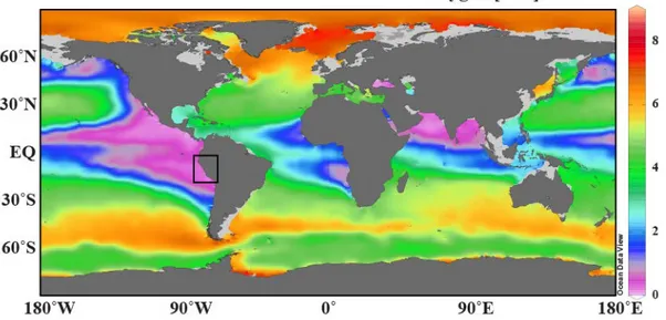
The present study, taking part in the second phase of the SFB and subproject B7, focused on question 3 and investigated the past variations in bottom water oxygen concentrations on a regional scale. Today, there are few places in the world oceans where these variations could be studied. The Peruvian margin is characterized by one of the most pronounced and persistent OMZs in the tropical oceans (Figure 1.1). Consequently, this study presents results obtained from sediment cores which were collected from the Peruvian margin in 2008 during expeditions M77 Leg 1 & Leg 2 aboard R/V Meteor. The main goal of the present study is a reconstruction of the bottom-water oxygen (BWO) concentrations for the last 22,000 years by using benthic foraminiferal assemblages.
Paleoceanographic and paleoclimatic reconstructions are needed for a better understanding of the changing climate, ocean and atmospheric circulation, hydrodynamics and the influence of all these changes on the living Earth. The elucidating past conditions would help us to formulize and model the future scenarios. Particularly investigating the last warming period (Termination I) at the end of the Last Glacial using marine sediment cores is crucial to obtain a sound understanding of today’s warming atmosphere and oceans. Thanks to their global distribution, quick response to environmental changes, and tests preserved in the fossil record,
2
benthic foraminifera have served as important tools in paleoceanography and paleoclimatology.
Their distributions in oxygen depleted environments have been matter of discussion and interest over the past decades. Some species were observed to be resistant to extremely low oxygen levels (e.g., Sen Gupta and Machain-Castillo, 1993; Bernhard and Sen Gupta, 1999; Gooday, 2003). Some of them have morphological features, such as pore structures, facilitating them to adapt to these extreme conditions (e.g., Piña-Ochoa et al., 2010; Glock et al., 2012b; Kuhnt et al., 2013). Certain species were used to assess the relative changes in the bottom water oxygenation during the last deglaciation at different parts of the Pacific Ocean (e.g., Moffitt et al., 2014;
Praetorius et al., 2015).
Figure 1. Global map showing the dissolved oxygen concentrations in the water column at 400 m water depths. The study area is depicted with a square; it is located in southern part of the Eastern Equatorial Pacific (EEP). Data is obtained from World Ocean Database, WOD2013 (Boyer et al., 2013).
In order to understand the recent processes and to create calibration datasets for downcore applications regarding to all these motivations mentioned above, surface sediment samples and cores were collected with a Multi-Corer, MUC from the Peruvian margin during the first phase of the project SFB754 in 2008. The living (rose Bengal stained) benthic foraminiferal distributions, taxonomy and morphological characteristics developed under the prevailing bottom-water conditions (e.g., oxygen concentrations) were previously documented as Ph.D.
theses and related articles (Glock, 2011; Glock et al., 2011; Mallon, 2012; Mallon et al., 2012).
To accomplish this dataset, living benthic foraminiferal faunas from 12 additional stations were included (Peréz et al., unpublished; Cardich et al., 2015). Using this information, the present study presents a comprehensive dataset of the benthic foraminiferal distribution along the
3
continental shelf and slope and attempts a reconstruction of their dynamics in relation with changing BWO concentrations.
The application to the fossil record mainly considers sediment cores recovered from the lower boundary of today’s OMZ in order to investigate potential changes in shape and extension of the OMZ during the deglaciation, and to quantify past oxygen levels. The main aims of the study were to: 1) to assess the stratigraphies of previously disregarded sediment cores and to combine the new information with existing cores, 2) to extent the knowledge and provide additional information on potential changes in bottom-water oxygenation such as total organic carbon accumulation, 3) to accomplish the benthic foraminiferal taxonomy of the sediment cores and to reconstruct past BWO levels using a benthic foraminiferal quantification approach based on the living-foraminifera dataset.
1.2. Outline
In addition to the motivation and previous works, Chapter 1 gives information on the study area, the present hydrodynamics and sedimentological characteristics of the Peruvian margin. A brief introduction on benthic foraminifera from the Peruvian margin and other Oxygen Minimum Zones is also included in this chapter.
In Chapter 2, basic information and stratigraphies of the sediment cores used for this study are described. Detailed information on cores, methods and materials used can be found in this chapter. Information given here is already published by (Schönfeld et al., 2015) and Erdem et al. (2016). It is used in preparation of different chapters of this thesis.
Chapter 3 presents a published paper (Erdem et al., 2016). The publication combines stratigraphical information from literature and the results from the new sediment cores. A ubiquitous hiatus and gaps in stratigraphical record were found in sediment cores from the Peruvian margin indicating an evolving structure since the LGM. The present publication focuses on the potential reasons of this non-deposition considering the present hydrodynamics of the region such as tide-topography interactions and non-linear internal wave formations and the impact of the Peru-Chile Undercurrent (PCUC) on the seabed and sediment transport.
Chapter 4 presents the downcore distribution of the benthic foraminiferal assemblages in each core separately. It includes the results obtained from the benthic foraminiferal investigations emphasizing on the most abundant species with comparisons between different cores and time intervals. Taxonomic reference list with supporting real colour pictures and SEM images can be found in the Appendix.
4
Chapter 5 presents the extended dataset of the living (rose Bengal stained) benthic foraminifera from the Peruvian margin. It describes BWO quantification approach in details which was applied to four sediment cores from the region using the information described in Chapter 4. Estimated BWO concentrations were later compared with previous records from the Eastern Equatorial Pacific.
All results and findings of this study are summarized in Chapter 6.
1.3. Declaration of contribution
Chapter 2: Parts of the results reported in this chapter are already published in Schönfeld et al., (2015) in which Zeynep Erdem is one of the co-authors. This paper is not considered as part of this Ph.D. thesis.
Data acquisition: Zeynep Erdem, Nicolaas Glock; Age Models: Zeynep Erdem Chapter 3: Published manuscript
Idea: Zeynep Erdem
Data acquisition: Zeynep Erdem, Nicolaas Glock, data of present day hydrodynamics by Marcus Dengler, Stefan Sommer, Thomas Mosch, seismic profile processing and interpretation by Judith Elger
Interpretation: Zeynep Erdem with major input from Joachim Schönfeld and Marcus Dengler Manuscript preparation: Zeynep Erdem with comments from co-authors.
Chapter 4: Draft manuscript
Idea: Zeynep Erdem, Joachim Schönfeld Data acquisition: Zeynep Erdem
Interpretation, manuscript preparation: Zeynep Erdem, with comments from Joachim Schönfeld Chapter 5: Draft manuscript (in preparation for submission)
Idea: Zeynep Erdem, Joachim Schönfeld
Data acquisition: Zeynep Erdem and input from co-authors regarding to their earlier works.
Methodology, Interpretation, Manuscript preparation: Zeynep Erdem with major in put from Joachim Schönfeld and with comments from co-authors.
5 1.4. Study Area
The Eastern Equatorial Pacific (EEP) comprises the tropical and subtropical areas off the western coasts of North and South America (Wyrtki, 1967; Kessler, 2006). This study focuses in particular on the southern part of the EEP offshore Peru and southern Ecuador, comprising the region between 1° and 18°S (Figure 1.1). The Peruvian coastal region is characterized by wind driven upwelling of cold and nutrient-rich water masses creating one of the most pronounced OMZs in today’s world oceans. The strength and extension of the Peruvian OMZ is maintained by the combination of a sluggish ocean circulation and high primary productivity in the surface mixed layer, leading to increased organic carbon export and enhanced consumption of dissolved oxygen in the water column (Wyrtki, 1962; Fuenzalida et al., 2009). The area regarded in this study comprises the continental shelf and slope off Peru and the southern part of Ecuador. It is characterized by an active continental margin with a narrow continental shelf up to 100 km width (Strub et al., 1998). A major part of the study area is under the influence of the Peruvian OMZ extending from 50 to 500 m water depth.
1.4.1. Present Hydrodynamics of the Eastern Equatorial Pacific
The EEP comprises the area between the California Peninsula in the North and Peru in the South where the North and South Pacific subtropical gyres move in which eastern boundary currents prevail, e.g., the California Current from north and the Peru Current from south (Fiedler and Talley, 2006). Most of the early oceanographic studies described the tropical Pacific, its currents, winds and thermal structure, only as function of latitude. For the EEP, the situation is different from open ocean settings, because the American continent on the eastern side of the region shapes the wind and circulation systems (Kessler, 2006; and the references therein).
There are two major current systems in the area; the Equatorial Current System (Wyrtki, 1967) and the Peru Current System (Gunther, 1936; Strub et al., 1998). The Equatorial Current System is composed of the westward-flowing near-surface South Equatorial Current (SEC), the Equatorial Undercurrent (EUC) and the primary and secondary Southern Subsurface Countercurrents (pSSCC and sSSCC) flowing eastwards underneath SEC (Figure 1.2; Montes et al., 2010). The SEC is a surface current that flows along Equator with a maximum velocity and shallowest thickness of 50 cm/s and 20 to 50 m. It gets thicker to around 200 m and slower further south extending to ~10°S in direction of west-southwest with irregular velocities (Wyrtki, 1967). The EUC is the northernmost subsurface current in the area and it flows underneath the SEC along the Equator (1.5°N to 1.5°S) between water depths of 30 and 200 m with maximum mean velocities of 20 to 30 cm/s (Montes et al., 2010). The Galapagos Islands act as a barrier for
6
the EUC splitting the current as north and south branches flowing around the islands. They merge again on the eastern side whereas a third branch flows southeastward converging with pSSCC at around 91°W (Figure 1.2; Karnauskas et al., 2007; Montes et al., 2010). The EUC water masses are characterized by high salinity, high nutrient content and oxygen depletion that make them a main nutrient source of the upwelling of the Peruvian OMZ (Strub et al., 1998).
Subsurface currents pSSCC and sSSCC flow eastwards at south of the EUC at 3-4°S and 6-8°S and with velocities of 5 cm/s and 15 cm/s, respectively (Figure 1.2; Montes et al., 2010).
Figure 1.2. Generalized map of the surface and subsurface current systems of South EEP (modified after Montes et al., 2010; Chaigneau et al., 2013); a) surface currents; SEC: South Equatorial Current; PCC: Peru Coastal Current; POC: Peru Oceanic Current, b) subsurface currents shown as dashed lines; EUC: Equatorial Undercurrent; pSSCC: primary Southern Subsurface Countercurrent; sSSCC: secondary Southern Subsurface Countercurrent; PCUC:
Peru‐Chile Undercurrent; PCCC: Peru‐Chile Countercurrent and CPDCC: Chile-Peru Deep Coastal Current.
The other major system, the Peru Current System is composed of the Peru Coastal Current (PCC) and the Peru Oceanic Current (POC) near the surface, the deep equatorward Chile-Peru Deep Coastal Current (CPDCC; Chaigneau et al., 2013), the Peru Chile Countercurrent (PCCC) and the Peru Chile Undercurrent (PCUC) in the subsurface, which is also called Gunther Undercurrent (GUC) (Figure 1.2; Montes et al., 2010). The northward
7
extension of the Humboldt Current originates from the Antarctic Circumpolar Current (ACC) and this northern flow splits off into PCC and POC at around 100-300 km offshore Chile (Mohtadi et al., 2005). The POC has a little contribution to the upwelling along the coast since it turns towards northwest to west at 24°S and is found until the water depths of 700 m (Wyrtki, 1967). In contrast, the PCC flows northward at much shallower depths due to upwelling processes along to coast. The PCC divert from the coast around 5°S and joins to the westward flowing SEC (Wyrtki, 1965). The CPDCC is flowing equatorward beneath the PCUC carrying cold and low salinity Antarctic Intermediate Water (Figure 1.3; Chaigneau et al., 2013; and the references therein). The equatorial subsurface water masses of PCCC and PCUC flow poleward beneath the surface currents at water depths of 100 to 400 m (Mohtadi et al., 2005) and they are fed by subsurface flowing EUC and SSCCs (Montes et al., 2010; Montes et al., 2011), thereby contributing to the coastal upwelling. The PCCC flows southward at 80°W and is strongest near 100 m depth but extends up to 500 m depth. It gets weaker and its transport decreases further south at around 22°S (Wyrtki, 1967). The characteristics of the PCUC were documented by in situ measurements (Brockmann et al., 1980; Huyer et al., 1991; Czeschel et al., 2011; Chaigneau et al., 2013), and approximated by modelling studies (Montes et al., 2010; Montes et al., 2011).
It originates at around 3-5°S as a shallow water mass and prevails from 50 to 300 m water depths. The PCUC prevails over the shelf and upper continental slope in the northern and central part of the region (Brockmann et al., 1980; Huyer et al., 1991; Czeschel et al., 2011). On its way south, it detaches from the continental slope south of 15°S but remains close to sea floor (Chaigneau et al., 2013).
Intermediate waters such as Antarctic Intermediate Water (AAIW) in the south of ~20°S and North Pacific Intermediate Water (NPIW) in the north of ~20°N are not the major water masses in the Eastern Equatorial Pacific (Fiedler and Talley, 2006). The low salinity (S<34.5) AAIW forms at the Subpolar Front by mixing of cold fresh Sub-Antarctic Mode Water (SAMW) and Polar Front waters (Sloyan and Rintoul, 2001). It spreads northwards up to Equator in the western part of the Pacific Ocean (Tsuchiya and Talley, 1996), whereas offshore Peru and below the Peruvian current system, the AAIW spreads northward arriving until 25-30°S at water depths between 500 and 1300 m (Figure 1.4; Fiedler and Talley, 2006). Below the AAIW, old and oxygen-poor Pacific Deep Water (PDW) extends towards the South (Fuenzalida et al., 2009).
The deepest water mass in the area is the northward spreading Antarctic Bottom Water (AABW;
Mohtadi et al., 2005).
8
Figure 1.3. The approximate positions of the PCUC and the CPDCC in relation with the sea- floor topography. Sea-floor profiles are modified after Suess et al. (1987), locations of the cores of the currents are after Chaigneau et al. (2013).
1.4.2. The Peruvian OMZ & Upwelling
In the southern part of the EEP, persistent, long shore south-easterly trade winds induce a westward offshore Ekman transport of surface waters. Warm waters accumulate in western Pacific elevating the sea level (Wyrtki and Wenzel, 1984) whereas in the area of the EEP, the eastward flowing undercurrents balance the pressure gradient caused by the elevated sea level in the west (Kessler, 2006). They bring cold and nutrient rich water masses and thereby sustain high productivity in the surface waters. Off Peru, these cold and nutrient rich waters rise from 50 to 350 m (mean depth of 130 m; Gunther, 1936) and reduce the surface water temperature by about 3°-4°C (e.g., Resig, 1990). The coasts of Peru and Chile are recognized as the most productive upwelling zone and ecosystem of today’s world oceans (Ryther et al., 1971;
Pennington et al., 2006). The most intense section of the Peruvian coastal upwelling is observed in the area between 5°S and 15°S reaching up to 100 km offshore and in particularly at 10°S to 15°S where the shelf becomes narrower. The strongest upwelling occurs in distinct cells in this section along the margin (Strub et al., 1998; Echevin et al., 2011; Mollier-Vogel et al., 2012).
9
Peruvian coastal upwelling is mostly seasonal because trade wind intensity is linked to the position of the Intertropical Convergence Zone (ITCZ), and reaches the maximum strength during southern hemisphere winter (Jun-Aug) (Pennington et al., 2006; Mollier-Vogel et al., 2013).
The whole region is characterized by not only high primary production but also by oxygen depletion in the water column due to decomposition of the organic matter. Sinking organic detritus is entrained by the PCUC, where the decay consumes oxygen in the water column. As oxygen advection is low and the flux of organic matter is high, excess oxygen consumption beneath the thermocline creates an extensive oxygen minimum zone (OMZ). The factors contributing the extreme oxygen deficiency in the EEP were considered as; (1) high production at the surface, (2) a sharp permanent pycnocline which obstructs the ventilation of subsurface water masses, (3) a sluggish deep circulation and thus limited advection of oxygenated deep waters from below the pycnocline (Kamykowski and Zentara, 1990; Helly and Levin, 2004; Fiedler and Talley, 2006). Identification of an oxygen depleted environment and classification of dissolved oxygen levels in these environments have been a matter of confusion and discussion. Kamykowski and Zentara (1990) presented their statistically treated data of dissolved oxygen concentrations in ml/l. Most of the following studies on oxygen minimum zones and oxygen depleted environments used this unit. Helly and Levin (2004) used a threshold value of <0.5 ml/l to estimate the coverage of OMZs in world oceans. The OMZs are also defined for dissolved oxygen concentrations of <20 µmol/kg (Fuenzalida et al., 2009) which is approximately 0.5 ml/l. The present study uses the unit µmol/kg as bottom-water-oxygen (BWO) concentration unit, and will report both values and units when necessary.
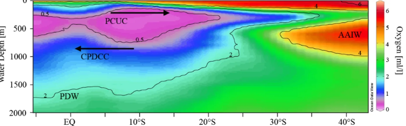
Figure 1.4. Latitude vs depth transect around 80°W showing the dissolved oxygen concentrations (1 ml/l = ~45 μmol/kg; WOD2013 (Boyer et al., 2013) and the principle water masses of the region (PCUC: Peru-Chile Undercurrent, CPCDCC: Chile-Peru Deep Coastal Current, AAIW:
Antarctic Intermediate Water and PDW: Pacific Deep Water).
10
The Peruvian OMZ has been estimated to cover ~34% of the total OMZ area in the world (in definition of hypoxia where dissolved oxygen levels of <0.5 ml/l; <20 μmol/kg prevail; Helly and Levin, 2004). Water masses and currents in the area regulate the thickness of the OMZ.
Distinct thinning occurs where the PCUC develop along the coastline whereas lower boundary depth of the OMZ also shows distinct latitudinal variations due to the influence of mid-depth circulation system in the region (Figure 1.4; Helly and Levin, 2004). The upper boundary of the Peruvian OMZ is located at 50-100 m water depth. Strong stratification below a very thin surface mixed layer extending to 50 m water depth limits the ventilation of the OMZ from above (Fuenzalida et al., 2009). The OMZ is around 500 m thick with marked oxygen minimum conditions (e.g., Strub et al., 1998; Fuenzalida et al., 2009). The core of the OMZ is centred off Peru to about 1000 km offshore between 5 and 13°S, where the upper boundary is shallow and the thickness reaches even 700 m (Figure 1.4). Further south towards the Chilean coasts and further north near the Equator, the thickness and the intensity of the OMZ decreases. Its boundaries extend along the Chilean coasts to about 37°S, driven by the southward flow of the PCUC along the continental margin (Fuenzalida et al., 2009). Seasonal or decadal changes in the position of the lower boundary are not expected but upper boundary may show inter-annual shifts of 65 to 100 m by changes in circulation as experienced during the 1997-1998 El Niño event (e.g. Helly and Levin, 2004).
1.4.3. Sediment distribution along the Peruvian margin
Late Quaternary sediments from the continental shelf and slope are predominantly olive green to dark grey green silt and clay. They show laminations within the OMZ whereas around the OMZ foraminifera bearing, bioturbated silty clays are found (Pfannkuche et al., 2011). At some levels coarse-grained sediments prevail which consist of foraminiferal sand (e.g., Oberhansli et al., 1990). South of 10°30’S, sediments from intense upwelling areas and within the OMZ are organic-rich diatom bearing silty clays which are occasionally laminated in places forming a 100 m thick, lens-shaped body on the gentle slope between 11 and 14°S (Krissek et al., 1980; Suess et al., 1987; Wefer et al., 1990; Pfannkuche et al., 2011). Terrigenous silts are found seaward south of 7°S, and grain size tends to decrease seaward as well (Krissek et al., 1980). The composition of the sand fraction is variable due to varying Andean detritus input.
Quartz and volcanic glass are abundant. Phosphorites that consist of hard grounds, crusts, nodules, pelletal grains and silt-sized grains (Manheim et al., 1975; Burnett, 1977; Glenn and Arthur, 1988) are abundant along the margin, particularly in Quaternary upwelling deposits (Garrison and Kastner, 1990). Ongoing phosphorite formation coincides with the upper and
11
lower boundaries of the OMZ (Burnett and Veeh, 1977). Widespread phosphorite hard grounds were also reported on the broad shelf north of 10°30’S (Reinhardt et al., 2002; Arning et al., 2009).
Sediments are typically composed of terrigenous material, organic matter (represented by TOC), carbonate (CaCO3), phosphorites and biogenic opal (Böning et al., 2004). In general, the southern sediments show lamination and high porosities (93-98%) because they are mainly composed of diatoms. Particulate organic matter (POC) values reach up to 15-20% (Neira et al., 2001; Levin, 2003). At the Peruvian continental margin, the highest organic carbon accumulation has been recorded on the shelf and upper slope at around 15°S as a result of high fluvial discharge by the Pisco River, intense oxygen minimum conditions and high surface water productivity. The shelf between 11 - 14°S is wider and the accumulation rates of organic matter are lower even though the organic carbon concentrations are higher (Reimers and Suess, 1983).
Further north offshore Ecuador, coarse calcareous biogenic debris dominates the shelf sediments (Krissek and Scheidegger, 1983). Towards the Chilean coasts, sedimentation rates show a distinct increase with reference to the higher detrital input (Muñoz et al., 2004). Sediments from upper slope do not show a distinct south-north difference in grain size whereas middle or lower slope sediments show a south-to-north fining in grain size due to the increase of seaward terrestrial input and winnowing (Krissek et al., 1980).
1.5. Micropaleontological proxies: benthic foraminifera
The overwhelming majority of modern foraminifera pursue benthic lifestyle and they constitute an extensive part in marine benthic ecosystems (e.g., Gooday, 2003). They are known for their fossil record reflecting environmental changes (e.g., Van der Zwaan et al., 1999;
Murray, 2006), such as temperature, surface productivity, bottom and pore water redox conditions etc. A well-documented recent distribution of benthic foraminiferal species and assemblage characteristics like population density and diversity provide background data for an interpretation of past bottom water conditions. Early investigators used benthic foraminifers as paleobathymetric indicators (e.g., Bandy, 1953a;b). Certain species were thought to be present at the same depth all over the world. Further studies showed that benthic foraminifera live not only at the surface of the sediment but also within the first 10 cm of the sediment (Corliss, 1985;1991). In the following years, studies focusing on the microhabitats showed that the faunal distributions and abundances are influenced and determined by the flux and temporal fluctuations of organic matter to the sea floor and the availability of the resources (e.g., oxygen) which result with mobilization of the foraminifera within the sediment (Barmawidjaja et al.,
12
1992; Loubere et al., 1993; Jorissen et al., 1995). However, later investigations revealed that the tolerance limits vary amongst species and certain species may occur in different sediment depths under conditions as predicted limiting factors (e.g., Sen Gupta and Machain-Castillo, 1993;
Bernhard et al., 1997). Using benthic foraminiferal assemblages as proxies for certain environmental parameters is an ongoing debate (Van der Zwaan et al., 1999; Gooday, 2003;
Jorissen et al., 2007), however, by investigating the environmental niches which determine the benthic foraminiferal assemblages in certain regions, it is possible to reconstruct the changes in the environmental conditions. With the increasing number of investigations on the living (stained) benthic foraminiferal assemblages, paleo-reconstructions are getting further.
1.5.1. Benthic foraminifera in oxygen depleted habitats
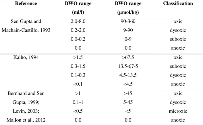
As mentioned earlier, the classification of the oxygen depleted environments, terminology for different oxygen levels and the units used for oxygen concentrations has been under debate (Table 1.1). Furthermore, Jorrisen et al. (2007) used the term hypoxic for all the environments where foraminiferal assemblages are potentially influenced without setting a specific value for a threshold oxygen level. In addition to the classification; certain thresholds are reported having negative impacts on marine organisms and ecosystems; oxygen levels <70 µmol/kg for some large macro-organisms (Stramma et al., 2010) and for meiofaunal abundance and diversity (Wetzel et al., 2001), which is defined as hypoxic environment, whereas 50 µmol/kg is reported as an onset for certain organisms and ecosystems which need specific physiological adaptations to abide (Seibel, 2011). Oxygen levels of 22 µmol/kg are used as a threshold for indicating the center of the OMZs (Helly and Levin, 2004; Fuenzalida et al., 2009), and laminated sediments are observed at oxygen levels are 7 µmol/kg where macrofauna is absent (Schönfeld et al., 2015). This study recognizes the above mentioned thresholds and uses the following terms and classification; oxic, dysoxic, microxic and anoxic with ranges of >45 µmol/kg, 5-45 µmol/kg, <5 µmol/kg and absence of dissolved oxygen, respectively.
Oxygen depleted environments are usually characterized with high organic matter flux to the sea floor. These two ecological factors, organic flux to sea floor and bottom-and pore-water oxygenation, are known to be the principal factors to control the benthic foraminiferal abundances and microhabitats (e.g., Lutze and Coulbourn, 1984; Corliss and Emerson, 1990;
Kaiho, 1994; Loubere, 1994; Alve and Bernhard, 1995; Loubere, 1996; Ohga and Kitazato, 1997; Altenbach et al., 1999; Gooday and Rathburn, 1999; Fontanier et al., 2003; Geslin et al., 2004). According to a proposed conceptual model, the microhabitat depth of endobenthic foraminifera in the sediment is controlled by the availability of food in oligotrophic
13
environments whereas oxygen concentration in the sediment controls the living depth of the species in eutrophic environments (Barmawidjaja et al., 1992; Jorissen et al., 1995). In most continental margin environments, the oxygen penetration depth within the sediments rarely exceeds 5 cm and vary between mm and first 10 cm (Reimers et al., 1992; Cai and Sayles, 1996).
Furthermore, certain deep infaunal species are also observed below the oxygen penetration depths, hence in anoxic sediments (e.g., Corliss and Emerson, 1990; Rathburn and Corliss, 1994;
Bernhard and Alve, 1996; Schönfeld, 2001; Koho et al., 2008) indicating that oxygen is not always the limiting factor determining benthic foraminiferal living depths. Consequently, certain species are found to be tolerant to extreme low oxygen levels which suggest that their distributions could be used as indicators of oxygen-depleted conditions (e.g., Sen Gupta and Machain-Castillo, 1993; Bernhard et al., 1997; Kaiho, 1999).
Table 1.1. Classification of different environments and thresholds of bottom-water-oxygen for benthic foraminifera and benthic biota in general.
Reference BWO range (ml/l)
BWO range (μmol/kg)
Classification
Sen Gupta and Machain-Castillo, 1993
2.0-8.0 0.2-2.0 0.0-0.2 0.0
90-360 9-90
0-9 0.0
oxic dysoxic suboxic anoxic Kaiho, 1994 >1.5
0.3-1.5 0.1-0.3
<0.1
>67.5 13.5-67-5
4.5-13.5
<4.5
oxic suboxic dysoxic anoxic Bernhard and Sen
Gupta, 1999;
Levin, 2003;
Mallon et al., 2012
>1 0.1-1
<0.5 0.0
>45 5-45
<5 0.0
oxic dysoxic microxic
anoxic
The consumption of oxygen is a restrictive factor for the average size of a species in areas with oxygen depleted bottom water conditions (Loubere, 1994). High population densities and a low diversity of benthic foraminifera have been documented by several studies in oxygen depleted environments (Phleger and Soutar, 1973; Sen Gupta and Machain-Castillo, 1993;
Bernhard et al., 1997; Jannink et al., 1998; Bernhard and Sen Gupta, 1999; Gooday et al., 2000;
14
Gooday, 2003; Koho and Piña-Ochoa, 2012; Mallon et al., 2012; Caulle et al., 2014). Absence of predators, such as the epifaunal gastropod Mitrella permodesta (Bernhard and Reimers, 1991), and competitors is also advantage for the assemblages in oxygen-depleted environments (Phleger and Soutar, 1973; Neira et al., 2001; Levin et al., 2002; Levin, 2003). There have been several studies which focused on specific benthic foraminiferal response to different oxygen levels.
Laboratory experiments were performed (e.g., Moodley et al., 1997; Geslin et al., 2004) or in situ observations were made, which focused on the Arabian Sea and the Indian Ocean (Hermelin and Shimmield, 1990; den Dulk et al., 1998; Jannink et al., 1998; Gooday et al., 2000;
Schumacher et al., 2007; Caulle et al., 2014), off Namibia (Leiter and Altenbach, 2010) and the Eastern Pacific Ocean (Smith, 1964; Phleger and Soutar, 1973; Douglas and Heitman, 1979;
Mullins et al., 1985; Mackensen and Douglas, 1989; Bernhard et al., 1997; Mallon et al., 2012;
Cardich et al., 2015). All these studies depicted a well-defined suite of hypoxia-resistant species.
It should be noted that most hypoxia-resistant species are also found in oxygenated environments at deep or intermediate endobenthic habitats (Sen Gupta and Machain-Castillo, 1993; Murray, 2001).
In general, most low-oxygen tolerant foraminifera are calcareous species (Gooday, 2003).
They are advantageous in environments with low oxygen and high organic matter as compared to the agglutinated species preferring oxygenated conditions and being less tolerant to hypoxic conditions (Bernhard and Sen Gupta, 1999; Gooday and Rathburn, 1999; Gooday et al., 2000;
Levin et al., 2002). Studies also show that thin walled species have advantages in oxygen depleted environments (e.g., Bolivina spp., Globobulimina spp.; Phleger and Soutar, 1973;
Kaiho, 1994). They are often characterized by elongate or flattened morphologies (Gooday, 2003). Another morphological feature is that these thin walled calcareous species generally have higher pore densities and pore-sizes in oxygen-depleted habitats as compared to oxic settings (Kaiho, 1994; Bernhard and Sen Gupta, 1999; Piña-Ochoa et al., 2010; Glock et al., 2011; Kuhnt et al., 2013). The most common species observed in the OMZs worldwide are Bolivina species (such as B. costata, B. seminuda, B. spissa), Globobulimina species (G. affinis, G. pacifica), Nonionella species (N. stella, N. turgida), Bulimina species (B. marginata, B. exilis), Buliminella species (B. elegantissima, B. tenuata), Cassidulina (C. delicata) species, and a few others (Sen Gupta and Machain-Castillo, 1993; Bernhard and Sen Gupta, 1999; Jorissen et al., 2007;
Schumacher et al., 2007). Experimental results of Moodley et al. (1997) showed that Nonionella and Stainforthia species survived longer under anoxic conditions than in oxic settings. Although they did not show reproduction, they seemingly could stand oxygen-depleted environments.
Certain agglutinated species such as Reophax spp., Trochammina spp., Adercotryma spp. are
15
also found in modern OMZs but they are not tolerant to intense oxygen depletion (Gooday, 2003).
1.5.2. Benthic foraminifera of the Eastern Equatorial Pacific OMZs
Several studies documented the benthic foraminiferal distribution off the Eastern Pacific coasts. Most of the works focused on the North American Coasts, in particular California borderland basins (e.g., Uchio, 1960; Douglas and Heitman, 1979; Mullins et al., 1985;
Mackensen and Douglas, 1989; Silva et al., 1996; Bernhard et al., 1997; Gooday and Rathburn, 1999; Rathburn et al., 2001). The Peruvian and Chilean fauna was documented by (Bandy and Rodolfo, 1964; Phleger and Soutar, 1973; Khusid, 1974; Ingle et al., 1980; Resig, 1981;1990;
Schönfeld and Spiegler, 1995; Figueroa et al., 2005; Morales et al., 2006; Tapia et al., 2008;
Cardich et al., 2012; Mallon, 2012; Mallon et al., 2012; Cardich et al., 2015). Some of the studies focused on living benthic foraminifera, but most of them concern dead assemblages. Sediments underneath the Peruvian OMZ support a high population density (Sen Gupta and Machain- Castillo, 1993; Mallon et al., 2012; Cardich et al., 2015, Pérez et al., unpublished). As observed in many oxygen depleted environments, an inverse correlation between diversity and population density was observed at the Peruvian OMZ. Overall, species of the family Bolivinitidae are tolerant to the dypoxic and microxic conditions (Phleger and Soutar, 1973; Khusid, 1974;
Manheim et al., 1975; Ingle et al., 1980; Resig, 1981;1990; Heinze and Wefer, 1992; Mallon et al., 2012; Cardich et al., 2015). The most common species observed in the region by all the studies mentioned are; Bolivina costata, B. interjuncta, B. spissa, B. seminuda, B. plicata, Globobulimina pacifica and Uvigerina peregrina.
Early studies subdivided the distributions of foraminifera assemblages in relation to water depths (e.g., Resig, 1981), whereas later studies focused on factors like food availability and oxygen concentrations. The assemblages are characterized by low-oxygen tolerant Bolivina species (Resig, 1981; Cardich et al., 2015). In particular, B. costata is dominating on the mid-to outer shelf and becomes rare below 150 m to about 500 m water depth (Resig, 1990; Cardich et al., 2012; Mallon et al., 2012; Cardich et al., 2015). Mallon et al. (2012) unveiled that not all of the species of the Boivinitidae family are tolerant to oxygen depleted conditions in the same way. Each species has its own tolerance limits to oxygen depletion. For instance, Bolivina seminuda is found everywhere whereas Bolivina costata is restricted to shallow, upper bathyal of the margin and Bolivina spissa are much more abundant outside of the OMZ core, giving an example of “ecological partition” between B. seminuda and B. spissa. Their occurrence in different depths indicated different oxygen and food demands. Additionally, Glock et al. (2011)
16
showed that B. seminuda is better adapted to oxygen depleted environments as compared to B.
spissa. General trends indicate that, food availability and increased values of oxygen concentration at the lower OMZ boundary make this environment rich in species. Especially some opportunists are absent within the OMZ, such as Angulogerina angulosa, U. peregrina, Bolivinita minuta (Mallon et al., 2012). The proportions of the agglutinated species also increase with water depth (Resig, 1981; Pérez et al., unpublished) and increasing bottom-water oxygen concentration (Mallon et al., 2012). Common taxa include Reophax spp., Eggerella spp., Rhizammina spp., Saccamina spp. and Trochammina spp. (Pérez et al., unpublished). High food availability in oxygen depleted conditions creates a less competitive environment so that certain species tolerating these extreme conditions could attain high densities (e.g., Gooday, 2003;
Jorissen et al., 2007). It is also known that some species mentioned before, use alternative metabolic pathway in the absence of oxygen (Risgaard-Petersen et al., 2006; Piña-Ochoa et al., 2010; Glock et al., 2012b; Koho and Piña-Ochoa, 2012; Fontanier et al., 2014).
17
2. METHODOLOGY AND STRATIGRAPHIES OF THE SEDIMENT CORES The present study focuses on
nine sediment cores obtained in 2008 during SFB754 expeditions M77 Leg 1
& 2 aboard R/V Meteor. Selection of the core locations was accomplished by sediment-echosounder profiling and bathymetric surveying during the expeditions (Pfannkuche et al., 2011).
They were located at continental slope of the Peruvian margin covering an area between 3°S and 18°S from water depths of 270 m to 1300 m (Table 2.1, Figure 2.1 and Figure 2.2). Four of these sediment cores were described earlier and their stratigraphic information were previously published (Mollier-Vogel, 2012; Mollier-Vogel et al., 2013). This chapter reports the stratigraphical information gathered from the remaining five cores which were used in different publications (Schönfeld et al., 2015; Erdem et al., 2016) (Chapter 3).
The sediment cores are stored in cold storage room of GEOMAR Kiel.
The sediment cores were split half, described and preliminary information was gathered on board. Measurements of the sediment lightness (L*) were done at every sediment core whereas the magnetic susceptibility (SI) measurements were only available for the short gravity cores obtained during M77 Leg 1. For details of the preliminary analyses on the sediment cores which were obtained during the expeditions, see the cruise report (Pfannkuche et al., 2011). The working halves of the sediment cores concerning this study were later sampled in the laboratory with 10 cm resolution up to 20 cc samples and 10 cc parallel samples (except core 47-2; this core was sampled previously by others). The 20 cc sample series were wet-sieved using a 63 μm sieve Figure 2.1. Map of the research area: red stars show the locations of the sediment cores which described in the present study for the first time and the black rounds show the core locations from the previous studies. See Figure 2.2 for the core locations in relation with the OMZ.
18
Figure 2.2. Depth vs latitude section showing the dissolved oxygen concentrations and the core locations as in Figure 2.1. Red stars show the locations of the sediment cores which described in the present study for the first time and the black rounds show the core locations from the previous studies. Oxygen data were taken from a CTD compilation after Schönfeld et al. (2015).
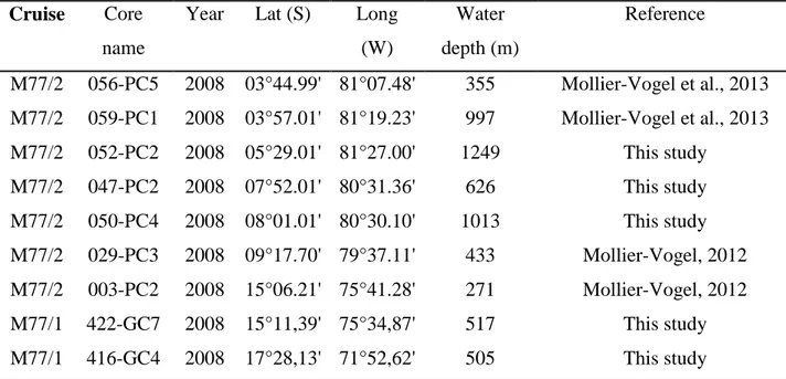
Table 2.1. The metadata of the sediment cores used in this study.
and residues were dried in 40°C oven. The sieved dry samples were later used for microfossil, sand-fraction examinations and further analyses such as; isotope analyses, radiocarbon dating.
The other series of the 10 cc samples were freeze dried and used for determination of physical properties such as dry bulk density and pore density (physical properties for core M77/2-47-2 were not available). All this information was later used in order compare and correlate the sediment cores and for the calculation of the accumulation rates. Additional to the physical Cruise Core
name
Year Lat (S) Long (W)
Water depth (m)
Reference
M77/2 056-PC5 2008 03°44.99' 81°07.48' 355 Mollier-Vogel et al., 2013 M77/2 059-PC1 2008 03°57.01' 81°19.23' 997 Mollier-Vogel et al., 2013 M77/2 052-PC2 2008 05°29.01' 81°27.00' 1249 This study
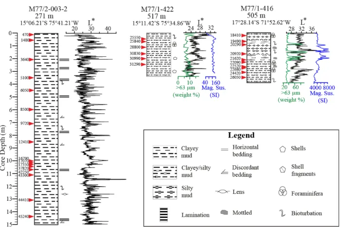
M77/2 047-PC2 2008 07°52.01' 80°31.36' 626 This study M77/2 050-PC4 2008 08°01.01' 80°30.10' 1013 This study M77/2 029-PC3 2008 09°17.70' 79°37.11' 433 Mollier-Vogel, 2012 M77/2 003-PC2 2008 15°06.21' 75°41.28' 271 Mollier-Vogel, 2012 M77/1 422-GC7 2008 15°11,39' 75°34,87' 517 This study M77/1 416-GC4 2008 17°28,13' 71°52,62' 505 This study
19
properties, subsamples of 3 to 20 mg dried samples from cores M77/2-50-4 and 52-2 were used for total nitrogen (TN), total carbon (TC) and organic carbon (TOC) content with a Carbon Erba Element Analyzer (NA1500) at GEOMAR, Kiel. The long-term precision was ±0.6 % of the measured values as revealed by repeated measurements of two internal carbon standards. Results regarding to total organic carbon were reported in Schönfeld et al. (2015).
2.1.Age models of the sediment cores
Oxygen (δ18O) and carbon (δ13C) isotope analyses were accomplished using a Thermo Fisher Scientific 253 Mass Spectrometer coupled to a CARBO KIEL automated carbonate preparation device at GEOMAR, Kiel. For the analysis, three to six specimens of the benthic foraminifera species Uvigerina peregrina, U. striata and Globobulimina pacifica were picked out from the >63 μm residues, according to availability. The results were reported in per mil (‰) relative to the VPDB (Vienna Pee Dee Belemnite) scale and calibrated versus NBS19 (National Bureau of Standards) and to an in-house standard (Solnhofen limestone).
The 14C Accelerator Mass Spectrometer (AMS) radiocarbon datings were performed at Beta Analytic, Inc., Florida, USA. For each dating point, from the >63 μm size fraction 229 to 250 specimens of the planktonic foraminifera species Neogloboquadrina dutertrei were picked.
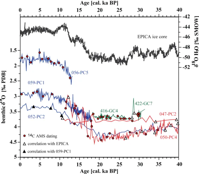
We were able to use N. dutertrei only in the sediment cores from the northern part of the region while in the southern cores this species was either absent or rare. In samples from the southern cores, from the >63 μm size fraction 33 to 179 specimens of Planulina limbata or 5 to 20 g of bulk sediment were used. Sedimentary organic carbon and foraminifera radiocarbon ages revealed a systematic offset of ~900 years, which was also observed and reported previously (Mollier-Vogel, 2012). Conventional radiocarbon datings were later calibrated applying the marine calibration set Marine 13 (Reimer, 2013) and using the software Calib 7.0 (Stuiver and Reimer, 1993). Reservoir ages ranging from 89 to 338 years for this region were taken into account according to the marine database (http://calib.qub.ac.uk/marine/). Ages are expressed in thousands of years (ka) before 1950 AD (abbreviated as cal ka BP; Table 2.2). The radiocarbon based chronologies for each sediment core were formed by linear interpolating the radiocarbon results. The chronologies of the cores were later supplemented and tuned using AnalySeries software with the Antarctic EPICA δ18O reference stack (EPICA Community Members Members, 2006). These results were later compared to the previously published age models and benthic δ18O records of the northern cores M77/2-56-5 and 59-1 (Figure 2.3.; Mollier-Vogel et al., 2013; Nürnberg et al., 2015). Core specific information regarding to the age models and reservoir ages are given in details below. Once the age models were complete and sedimentation
20
rates were calculated, accumulation rates (ARbulk (g/cm² ka)) were calculated following (Van Andel et al., 1975) for each core by using the dry bulk densities gathered from the physical property measurements.
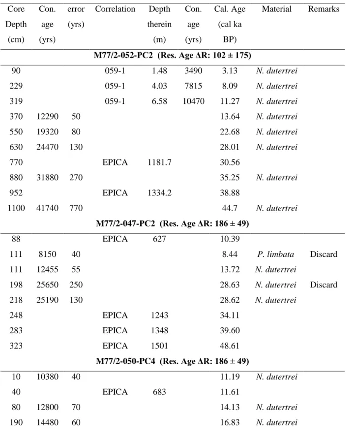
Table 2.2. Age models of the five sediment cores listed in accordance to their location (from north to south).
Core Depth
(cm)
Con.
age (yrs)
error (yrs)
Correlation Depth therein
(m)
Con.
age (yrs)
Cal. Age (cal ka
BP)
Material Remarks
M77/2-052-PC2 (Res. Age ΔR: 102 ± 175)
90 059-1 1.48 3490 3.13 N. dutertrei
229 059-1 4.03 7815 8.09 N. dutertrei
319 059-1 6.58 10470 11.27 N. dutertrei
370 12290 50 13.64 N. dutertrei
550 19320 80 22.68 N. dutertrei
630 24470 130 28.01 N. dutertrei
770 EPICA 1181.7 30.56
880 31880 270 35.25 N. dutertrei
952 EPICA 1334.2 38.88
1100 41740 770 44.7 N. dutertrei
M77/2-047-PC2 (Res. Age ΔR: 186 ± 49)
88 EPICA 627 10.39
111 8150 40 8.44 P. limbata Discard
111 12455 55 13.72 N. dutertrei
198 25650 250 28.63 N. dutertrei Discard
218 25190 130 28.62 N. dutertrei
248 EPICA 1243 34.11
283 EPICA 1348 39.60
323 EPICA 1501 48.61
M77/2-050-PC4 (Res. Age ΔR: 186 ± 49)
10 10380 40 11.19 N. dutertrei
40 EPICA 683 11.61
80 12800 70 14.13 N. dutertrei
190 14480 60 16.83 N. dutertrei
21
250 15370 60 17.98 N. dutertrei
350 17690 70 20.62 N. dutertrei
450 18750 70 22.01 N. dutertrei
550 20330 90 23.72 N. dutertrei
824 EPICA 1114 26.97
1010 25680 130 29.12 N. dutertrei
1190 29030 170 32.39 N. dutertrei
1302 EPICA 1245 34.11
1461 EPICA 1288 36.57
1745 EPICA 1370 40.86
M77/2-422-GC7 (Res. Age ΔR: 338 ± 186)
31.5 21950 90 25.55 Sediment
77 22300 90 25.84 Sediment
122 25510 120 28.80 Sediment
145 EPICA 1151 29.48
154 EPICA 1160 29.79
168 27320 140 30.83 Sediment
212 27610 140 30.99 Sediment
257 28200 150 31.29 Sediment
275 EPICA 1181 31.52
307 19350 70 22.50 Sediment Discard
M77/2-416-GC4 (Res. Age ΔR: 338 ± 186)
20 15900 60 18.41 P. limbata
35 406 16 16320 18.83 P. limbata
45 406 23 16600 19.14 P. limbata
60 16910 70 19.49 P. limbata
100 17690 80 P. limbata Discard
110 17560 80 20.29 P. limbata
160 18080 90 20.92 P. limbata
210 18610 80 21.62 P. limbata
230 18970 80 22.09 P. limbata
245 19370 90 22.52 P. limbata
250 19550 100 22.68 P. limbata
290 18930 90 P. limbata Discard
22
310 21050 130 24.42 P. limbata
345 22560 120 26.05 P. limbata
2.2. Core specific information Core M77/2-052-PC2
The M77/2-052-PC2 is a long piston core and here referred as 52-2. It was collected from the northern part of the region and from 1249 m water depths. The sediment core is composed of homogeneous olive green grey mud with no significant change in sedimentological characteristics (Figure 2.5). The weight percentages of >63 μm determinations and information on sediment surface lightness (L*) showed a change around 5 m core depth, indicating higher porosity, less sandy and darker material for the topmost 5 m. For the δ18O and δ13C measurements benthic foraminifera Uvigerina peregrina were picked. Benthic δ18O values ranged between 3.083 and 4.755 (Figure 2.3), whereas benthic δ13C values ranged between - 1.115 and -0.037 (Figure 2.4). Radiocarbon dating of this core was done by 5 dating points using the planktonic foraminifera Neogloboquadrina dutertrei. This species were rare at the first 3 m of the core, so we were unable to date the core for these depths. We recognized a good correlation between δ18O curves of the core 52-2 and 59-1, therefore the age model was accomplished by correlation to core 59-1 for the Holocene part and tuned by correlation to EPICA ice-core for the later periods (Figure 2.3). It covers whole period of 40 ka without gaps and disturbances in the downcore record. Sedimentation rates for the last 25 ka ranged between 11 and 28 cm ka-1 (Figure 2.6). Total nitrogen (TN), total carbon (TC) and total organic carbon (TOC, Corg) measurements were accomplished with 10 cm resolution for the first 700 m of the core 52-2. The CaCO3 (%) values were calculated using the values TC (%) and TOC (%).Total organic carbon values ranged between 1 and 3 % showing a distinct slight increase starting from 390 cm (~14 cal ka BP), whereas CaCo3 values ranged between 1 and 7 %, showing similar trend with >63 μm (weight %) of this core. A distinct drop was observed between core depths of 450 cm and 500 cm (17 and 20 cal ka BP). Total nitrogen percentages (TN (%)) were in accordance with TC (%). The accumulation rates of N (ARN) and Corg (ARCorg) were calculated accordingly.
23
Figure 2.3. Benthic δ18O isotope curves of the sediment cores with age control points. Graphs are depicted in different colours regarding to the core locations; blue for the northern cores, red for the central and green for the southern cores.
Core M77/2-050-PC4
The M77/2-050-PC4 is a long piston core and is here referred as 50-4. It was collected from the central part of the region and from 1013 m water depths. The sediment core is composed of olive green to olive green grey homogeneous mud bearing foraminifera throughout the core. There are some changes in the sediment colour and some laminas are also observed but these are not continuous and distinct differences. The >63 μm weight % values showed a similar change to core 52-2 around 2 m core depth. Lightness (L*) did not show such a similarity (Figure 2.5). For the δ18O and δ13C measurements of the core 50-4, benthic foraminifera species Uvigerina peregrina and Globobulimina pacifica (only for the first 4 m of the core, not shown here) were used. Benthic δ18O values ranged between 2.896 and 4.655 (Figure 2.3), whereas benthic δ13C values ranged between -3.679 and -0.117 (Figure 2.4).