A mobile, high-precision atom-interferometer and its application to gravity observations
D I S S E R T A T I O N
zur Erlangung des akademischen Grades doctor rerum naturalium
(Dr. rer. nat.) im Fach Physik eingereicht an der
Mathemathisch-Naturwissenschaftlichen Fakultät Humboldt-Universität zu Berlin
von
Dipl.-Phys. Matthias Hauth
Präsident der Humboldt-Universität zu Berlin:
Prof. Dr. Jan-Hendrik Olbertz
Dekan der Mathemathisch-Naturwissenschaftlichen Fakultät:
Prof. Dr. Elmar Kulke Gutachter:
1. Prof. Achim Peters, Ph.D.
2. Prof. Dr. Oliver Benson 3. Prof. Dr. Holger Müller
Tag der mündlichen Prüfung: 06.03.2015
Abstract
Atom interferometry offers a very precise and sensitive measurement tool for various areas of application whereof one is the registration of the gravity acceleration. While the vast majority of atom interferometers include large and stationary setups, this field very often implies the additional request for a mobile apparatus. The Gravimetric Atom Interferometer (GAIN) project has been started to meet this requirement and to provide best possible accuracy at the same time. It aims to realize an alternative to other types of gravimeters and to combine important qualities such as high sensitivity and absolute accuracy in one instrument.
The GAIN sensor is based on laser-cooled87Rb atoms in a 1 m atomic fountain. Stimulated Raman transitions form a Mach-Zehnder type interferometer which is sensitive to accelera- tions. In this work it has been advanced to meet all requirements for mobile and drift-free long-term operation. Therefore, selected parts of the laser system have been improved or redeveloped. A second focus has been on systematic effects for the same objective. They have been analyzed and measures for their suppression have been undertaken.
The apparatus has been transported, tested in relevant environments, and compared to the most important state-of-the-art gravimeter types where a competitive performance has been achieved. It is demonstrated, that the gravity signal of this sensor allows for a precise calibration of the relative gravimeter types. During the measurements a best sensitivity of 138 nm/s2/√
Hz and a stability of 5×10⁻¹¹g after 105s has been reached.
Zusammenfassung
Atom Interferometrie ist eine sehr genaue und sensitive Methode mit einer Vielzahl von Anwendungsmöglichkeiten, zu der auch die Messung der Erdbeschleunigung zählt. Wäh- rend die meisten Atom Interferometer aus großen, ortsfesten Aufbauten bestehen, werden auf diesem Gebiet häufig mobile Messgeräte benötigt. Das Gravimetric Atom Interfero- meter (GAIN) Projekt wurde ins Leben gerufen, um dieser zusätzlichen Anforderung bei bestmöglicher Messgenauigkeit gerecht zu werden. Es soll eine Alternative zu anderen mod- ernsten Gravimetertypen geschaffen werden, die wichtige funktionale Eigenschaften wie eine hohe Auflösung und absolute Genauigkeit in einem Gerät vereint.
Der GAIN Sensor verwendet lasergekühlte 87Rb Atome in einer 1 m hohen Fontäne. Mit Hilfe von stimulierten Raman Übergängen wird ein beschleunigungssensitives Interferometer realisiert. In dieser Arbeit wurde der Sensor mit Blick auf mobile und driftfreie Langzeitmes- sungen weiterentwickelt. Dafür wurden einzelne Subsysteme des Laseraufbaus auf die daraus resultierenden Anforderungen hin angepasst oder neu entwickelt. Mit derselben Zielstellung wurden weiterhin systematische Effekte in dem Messaufbau untersucht und Maßnahmen für ihre Reduzierung realisiert.
Der Aufbau wurde transportiert und in relevanten Umgebungen getestet. Dabei konnte gezeigt werden, dass die Leistungsfäigkeit dieses Aufbaus mit denen der wichtigsten und modernsten Gravimeter konkurieren kann, sie teilweise übertrifft und dass dieser Sensor zur präzisen Kalibrierung der relativen Gravimeter verwendet werden kann. In den Messungen wurde eine Sensitivität von 138 nm/s2/√
Hz sowie eine Langzeitstabilität von 5×10⁻¹¹g über 105s erreicht.
Contents
1. Introduction 1
1.1. Gravity and its variations on Earth . . . 2
1.2. Gravimeters based on atom interferometry . . . 5
1.2.1. Atom interferometry . . . 5
1.2.2. Working principle . . . 5
1.2.3. The Gravimetric Atom Interferometer (GAIN) . . . 7
1.3. Classical gravimeters . . . 7
1.3.1. Mechanical spring type gravimeters . . . 7
1.3.2. Superconducting gravimeters . . . 8
1.3.3. Laser interferometer absolute gravimeters . . . 9
1.3.4. Applications . . . 10
1.4. Organization of this thesis . . . 11
2. Theoretical background 13 2.1. Stimulated Raman transition . . . 13
2.2. Atom Interferometer . . . 19
2.2.1. Sensitivity function . . . 21
2.2.2. Phase noise due to laser phase noise . . . 22
2.2.3. Phase noise due to mirror vibrations . . . 25
2.2.4. Gravity gradient . . . 26
2.3. Interferometry with Rubidium 87 . . . 27
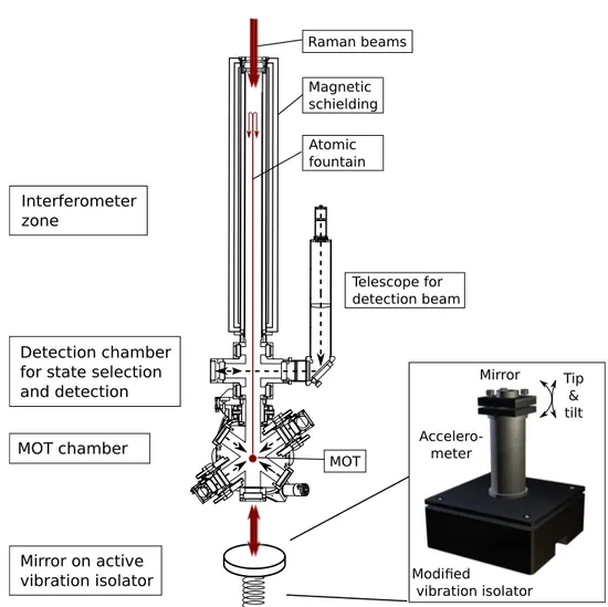
3. Experimental setup 31 3.1. Physics package . . . 32
3.1.1. Vacuum chamber . . . 32
3.1.2. Active vibration isolator . . . 34
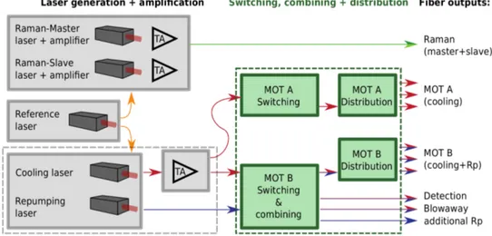
3.2. Laser system . . . 36
3.2.1. Laser frequencies and sources . . . 37
3.2.2. Modular setup . . . 38
3.2.3. Original switching module . . . 39
3.2.4. New switching modules . . . 41
3.2.5. Raman intensity stabilization . . . 45
3.3. Timing system and data storage . . . 47
4. Gravity measurement 51
4.1. Experimental sequence . . . 51
4.1.1. magneto-optical trap (MOT) and optical molasses . . . 51
4.1.2. Selection process . . . 53
4.1.3. Interferometer phase . . . 54
4.1.4. Detection . . . 55
4.2. Gravity measurement protocol . . . 57
4.3. Gravity . . . 58
5. Systematic effects 61 5.1. Coriolis effect of the Earth . . . 61
5.2. Tilt . . . 62
5.2.1. Alignment and active tilt stabilization of the reference mirror . . . 62
5.2.2. Tilt and alignment of the Raman telescope . . . 63
5.3. Reference frequencies . . . 65
5.3.1. Radio frequency reference . . . 66
5.3.2. Frequency of the reference laser . . . 66
5.4. Detection . . . 68
5.4.1. Shape of the detected fringe . . . 68
5.4.2. Arrival time of the atomic cloud . . . 70
5.5. Reversed Raman light vector . . . 70
5.6. AC-Stark shift . . . 72
5.7. Overview of systematic effects . . . 74
6. Gravity comparison campaigns 75 6.1. Comparison with the gPhone . . . 75
6.2. Comparison with the FG5X . . . 78
6.3. Comparison with the superconducting gravimeter . . . 80
6.3.1. Gravity recordings . . . 80
6.3.2. Long-term stability . . . 81
6.3.3. Scaling factor of the SG-30 . . . 83
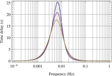
6.3.4. Time delay . . . 84
6.3.5. Amplitude spectral densities . . . 86
6.3.6. Absolute gravity value . . . 88
6.4. Mobility of the instrument . . . 88
6.5. Noise analysis . . . 89
7. Conclusion and perspectives 91
A. Tidal parameters 93
B. Raman intensity controller 97
C. Allan variance 99
Contents
D. Effect on gravity from atmospheric mass redistribution 101
E. Measurement in Wettzell 103
Bibliography 113
Publications 115
List of Figures 120
List of Tables 121
List of Abbreviations 124
Acknowledgments 126
1. Introduction
The gravitational force is one of four fundamental interactions in physics. Though it is about 1029 to 1038 times smaller than the electromagnetic, the weak, and the strong interaction, it plays an important role on macroscopic scales such as in the field of cosmology. But also in everyday life we are familiar with this force. All matter, including ourselves, fall back to Earth if not dominated by other forces. Observations done over the course of several hundred years led to a profound description of this force. Important milestone were the examinations of the free fall made by Galileo and his conclusion that all matter is accelerated at the same rate.
The first complete mathematical description was given by Sir Isaac Newton in his famous work
“Philosophiæ Naturalis Principia Mathematica” in 1687. Newton’s law of universal gravitation describes the attracting force Fg between any two bodies which is proportional to their masses m1 and m2
Fg=Gm1m2
r2 (1.1)
whereGdenotes the gravitational constant andrthe distance between the centers of the masses.
The gravitational force has some characteristic properties: It is always attractive, has infinite range, and it cannot be shielded. By now, Newton’s law of universal gravitation can be seen as an approximation of Einstein’s general theory of relativity which is the current theory of gravitation.
It holds very precise in the limits of low mass densities and non-relativistic velocities [1, 2].
Equation (1.1) includes four parts which have been, in parts intensively, investigated in the past and are still matter of ongoing research. These are:
The gravitational constant G has been measured by a large number of experiments but still is the fundamental constant with the by far largest inaccuracy [3, 4].
The inverse-square law describes the decreasing strength with the distance r between the masses. Possible violations have been tested on different length scales [4–6].
The gravitational acceleration ag =Fg/m1 ∝nm2,n/rn2 an object with massm1 is subjected to is the consequence of the gravitational force. The latter is determined by the distribution of all masses m2,n of the near and also the far environment at distances rn. Thus a precise investigation of this force or the corresponding acceleration gives the sum over all masses weighted with their distances. Temporal and spatial observations can allow to draw conclusions, e.g., on the mass distribution above and below the surface of the Earth and thereby on its composition [7–9].
The weak equivalence principle, also known as the universality of free fall (UFF) or as the Galilean equivalence principle, states that “the motion of any freely falling test particle is independent of its composition and structure” [2]. It is one important aspect of general
relativity. In combination with Newton’s second law of motion F =mia the equivalence between the inertial massmi and the gravitational mass of the test particlem1in Eq. (1.1) can be tested.
For studies of all four aspects of the gravitational law it is necessary to measure either the gravitational force Fg or the consequent gravitational acceleration ag which acts on the test mass m1. A variety of experimental apparatus have been developed during the last centuries to investigate one or the other. Atom interferometers are one of the newest devices which are among other things sensitive to accelerations. Here, their application to gravity observations, which include the aspect of the gravitational acceleration, will be covered.
1.1. Gravity and its variations on Earth
All matter on Earth is subjected to the gravitational acceleration. However, the acceleration which can be observed includes a second contribution which cannot be avoided. The Earth is a non-inertial reference frame because of its rotation and causes a centrifugal force
Fz=mω2d. (1.2)
Here, m denotes the observed mass, ω the rotation rate, and d the distance between the mass and the rotation axis of the Earth. The sum of both forces determines the acceleration all matter is subjected to. Throughout this thesis and in accordance with literature [8, 9] the term
“gravity acceleration” or shorter “gravity” will denote the combined effect of the gravitational acceleration and the centrifugal acceleration due to Earth’s rotation. The instruments used for measuring the gravity value are gravimeters.
Gravity acceleration is altered by a variation of influences in time and space. Global variations on Earth can already be visible at the second decimal place. The difference in gravity between, e.g., Berlin-Adlershof and Wettzell in the Bavarian Forest, two locations where measurement campaigns have been performed during this thesis, amounts to 4×10⁻⁴g. Regional variations, on the other hand, are typically on the order of 10−6g. Temporal influences are even slightly smaller. The largest one is the basic tidal effect reaching magnitudes of up to almost 3×10⁻⁷g, whereas the effects of mass redistributions in the atmosphere or below the surface of the Earth and also of man-made changes are again smaller.
An overview of the different effects and their magnitudes is given in Fig. 1.1. Short intro- ductions into the physics of the Earth tides and the interest in resolving the effect of mass redistribution are given in the following.
Tidal effect
The Earth is attracted by the gravitation arising from external bodies like the sun, the moon, and to a minor extend other planets. Due to the inverse-square law the resulting acceleration is non-homogeneous throughout the Earth but changes with position. On the other hand, the whole Earth underlies an orbital acceleration which is connected to its orbital motion. Both
1.1. Gravity and its variations on Earth
9 , 8 1 2 , 6 4 1 , 7 4 2 nm / s² 9 , 8 0 8 , 3 6 9 , 7 5 4 nm / s²
Regional variations Global variations
Basic tidal e ect
Mass redistribution (e.g., atmosphere)
People new Buildings
Adlershof:
Wettzell:
Figure 1.1.: Gravity acceleration measured within this work in Berlin-Adlershof and Wettzell (Bavaria). The values are influenced by a variety of effects causing changes at different decimal places which are indicated by the arrows.
accelerations exactly match at a certain point in general and for a spherical symmetric Earth in its center of mass. At other locations their difference gives a remaining tidal acceleration [9, 10].
The tidal effect is visualized in Fig. 1.2 for a simplified system with a non-rotating Earth and its Moon. Both bodies orbit around their common barycenter resulting in the Earth’s orbital acceleration which only coincides with the gravitational acceleration aO in the Earth’s center of mass O. At a point P located at the Earth’s surface the local gravitational acceleration a differs. Here, the difference of both accelerations results in the tidal acceleration at, which can be expressed using Newton’s gravitational law as
at=a−aO= GMm
d2 d
d −GMm
r2 r
r (1.3)
whereG,d, andrdenote the gravitational constant and the distances between pointO and the Moon and point P and the Moon respectively. As a result the tidal effect lowers gravity on the side of the Earth facing the Moon as well as on the opposite side and the acting forces cause elastic deformations of the Earth’s shape which can reach up to 40 cm.
In addition, a semidiurnal and diurnal variation is induced by the Earth’s rotation which then causes the well-known rise and fall of sea levels. The moving water masses themselves give an additional contribution to gravity variations by direct attraction (ocean tides) and also by loading effects which again cause elastic deformations of the Earth’s shape (ocean load tides).
The latter are subject to phase leads. Even more temporal variations are introduced by changing distances between the Earth and the Moon and between the Earth and the Sun as well as by seasons and lunar phases. All effects together result in a variety of semidiurnal, diurnal, and long-period tides.
Tidal effects can be calculated using theoretical models together with ephemerides of celes- tial bodies and local parameters obtained from former gravity observations, see Appendix A.
Thus, gravimetric measurements can be reduced for these dominating temporal effects and other influences become visible.
P
Moon undeformed
Earth
O
r d
-aO aO -aO
at
a
Figure 1.2.:Emergence of the tidal effect caused by the moon.
Polar motion
The Earth’s rotation axis is subjected to slight temporal variations of its orientation relative to the Earth’s surface. Their intersection points (poles) move several meters per year with periodic and long-term drift components. As a consequence the distance between a fixed location on the Earth’s surface and the rotation axis also evolves over time and thereby the resulting centrifugal acceleration undergoes temporal changes. The latter are typically within±50 nm/s2 in Northern Germany [12]. They can be calculated using Earth observation parameters from the International Earth Rotation and Reference Systems Service (IERS) and then be reduced from gravity observations.
Mass redistribution
Mass redistributions above as well as below the surface of the Earth occur due to a variety of causes. They change the local gravity acceleration according to Eq. (1.1) and their influence typically reaches magnitudes of a few times 10−8g. One important aspect is the influence of atmospheric mass variations which we were also able to observe during our measurements.
It causes gravitational attraction and also an additional loading effect. The latter vertically deforms the crust and mantle of the Earth. The atmospheric variations at the same time cause changes of the local air pressure which can be used in a simple model for corrections. Applying the correlation
gatm =aatm(p−p0) (1.4)
with the admittance factor aatm ≈3.0 nm/s2/hPa and the normal atmospheric pressure p0 for the specific height, the main part of the effect can be removed. Other mass redistributions are induced, e.g., by rainfall and hydrology. Here, observations with gravimeters can be of interest to get further insights and support other methods like water table observation wells. Beyond that general studies of mass convections below the surface of the Earth are of interest in geodynamics where amongst others magma transport and tectonic plate movements are investigated [13, 14].
Free air gravity gradient
The inverse square law in Eq. (1.1) causes the gravity value to decrease with the height h. This results in a vertical gravity gradient in free air of γ = ∂g∂h ≈3080 nm/s2/m near the surface of the Earth [9].
1.2. Gravimeters based on atom interferometry
1.2. Gravimeters based on atom interferometry
1.2.1. Atom interferometry
Atom interferometers were realized almost in parallel by different research groups in the early 1990s. They achieved the coherent splitting and recombination which are necessary to observe interference with the help of various experimental implementations. Two of the groups worked with micro-fabricated structures of which one was similar to Young’s double slit [15] and the second a transmission grating [16]. The other approaches used laser waves in a traveling wave configuration [17] and in a pulsed configuration with stimulated Raman transitions [18]. There- after, especially atom interferometers with laser waves as beam splitters had been increased in their sensitivities and were used for precise measurements of the fine structure constant [19, 20]
and of the gravitational constant [21–24]. The principle was also employed in different configura- tions for precise inertial sensors like gyroscopes [25–27], accelerometers and absolute gravimeters [28–30], and gravity gradiometers [31]. The latter are able to measure gravity gradients.
The experiments demonstrated that the possible sensitivities and absolute accuracies are competitive to state-of-the-art instruments which are based on different working principles. For gravimeters based on this principle, the best reported sensitivities so far are 230 nm/s2/√
Hz [29], 80 nm/s2/√
Hz [32], and recently for a measurement in a particular quiet seismic environment 42 nm/s2/√
Hz [33]. While most atom interferometers are constrained to fixed laboratories, several approaches have been started to develop mobile devices. The idea is to make inertial sensing based on atom interferometry applicable to, e.g., navigation and geophysics [34–36].
Further possible fields of application are fundamental precision measurements for testing gen- eral relativity [37–39]. Ground based tests of the UFF already achieved Eötvös ratiosη = ∆g/g of (1.2±3.2)×10−7 and (0.3±5.4)×10−7for the combinations85Rb−87Rb [40] and87Rb−39K [41] respectively. Studies for space missions propose to drastically increase the accuracy by several orders of magnitudes mainly due to extended times of free evolution between the in- terferometer pulses. Within several European Space Agency (ESA) projects a compact atom interferometry demonstrator (Space Atom Interferometer (SAI) project [42]) and further con- cepts for sensors in space (Space-Time Explorer and Quantum Equivalence Principle Space Test (STE-QUEST) [43, 44]) have already been developed. Another concept describes the pos- sibility to detect gravitational waves with the help of atom interferometers in space [45].
1.2.2. Working principle
The atom interferometer discussed in this work is based on stimulated Raman transitions [18]
which are applied to a cold ensemble of rubidium-87 atoms inside a ultra-high vacuum (UHV) chamber. The atoms are laser-cooled in a magneto-optical trap (MOT) and a subsequent optical molasses to about 2µK in order to realize low velocities and long observation times of the cloud of nearly 1 s. In comparison to a light interferometer the roles of light and matter are interchanged.
After preparation the atoms are coherently transferred to a superposition of two internal energy states with different external momenta. As a consequence the states evolve onto two different paths. Afterwards, they are redirected and finally recombined. The necessary beam splitters and mirrors are realized by means of laser light pulses which drive the atomic transitionωa between
time
height
Figure 1.3.: Mach-Zehnder type atom interferometer with three Raman light pulses (π/2−π−π/2 sequence). The first pulse creates a superposition of two internal states |g⟩ and |e⟩ with different momenta. They evolve onto separate paths. The second and third pulse reflect the paths and close the interferometer.
the two hyperfine states. Therefore, the frequency difference of two laser beamsω1−ω2 is tuned to be in resonance with the atomic transition. The single laser beams are not in resonance with any transition but near the D2 (52S1/2 → 52P3/2) transition at a wavelength of 780 nm. If an atom undergoes the Raman transition a photon of one light field is absorbed while at the same time the emission of another photon is stimulated by the other light field. This way energy and also momentum are transferred to or extracted from the atom depending on its initial state.
In a Mach-Zehnder type atom interferometer, which is used in this work, three Raman light pulses are applied, see Fig. 1.3. After the atoms have been prepared to be all in the same internal state, the first pulse transfers each of the atoms into a superposition of the two hyperfine states
|g⟩and|e⟩. Its light intensity and pulse length are tuned to reach equal probabilities of occupancy for both states (π/2 pulse). As a consequence the different states spatially separate, due to the transferred momenta, onto two paths. After a time T a second pulse with double length (π pulse) is applied. It inverts both the internal state and the external momentum the atoms have on the two paths. The latter meet again after another time T. The third pulse, which is again a π/2 pulse, finally closes the interferometer. The splitting between the paths and the phase sensitivity becomes maximal for counter-propagating laser beams.
At the output, interference can be observed. The resulting state population depends on the phase difference ∆ϕbetween the two paths and the probability of the atoms to be transferred to the other internal state is given by
P = 1
2(1−cos ∆ϕ). (1.5)
∆ϕ includes contributions from the exact paths in space as well as from the interaction of the atoms with the Raman laser pulses.
Atom interferometers can be used to measure influences on their phase very precisely. Depend- ing on the implemented configuration a variety of different effects, e.g., rotations or accelerations due to gravitational or other forces, can be observed. In order to use atom interferometers for
1.3. Classical gravimeters high-precision experiments it is necessary to obtain a very good control on laser phases and to suppress all but the desired influence to a sufficient level. A configuration with free falling atoms along the vertical direction and anti-parallel laser beams which are aligned along the same axis allows to measure gravity acceleration [28, 46]. The latter causes a phase shift of
∆ϕ≈keffgT2 (1.6)
where g is the gravity acceleration, keff the effective wave vector resulting from the Raman laser beams, and T the time between consecutive laser pulses. Equation (1.6) shows that it is favorable to realize long interferometer times T in order to increase the sensitivity of a setup.
1.2.3. The Gravimetric Atom Interferometer (GAIN)
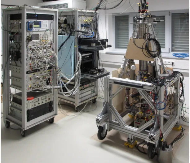
The GAIN experiment is an atom interferometer which has been designed to allow for high- precision gravity measurements at different locations. This field of application implicates much stronger and partly new requirements in comparison to experiments in optical laboratories.
Many parts, especially for the laser setup, have been redesigned in order to drastically shrink them in size and achieve a transportable sensor. Transportable in this context means that it can be transported by a small truck and moved around on wheels to the location of interest.
Other design criteria have been a fast recommissioning after transportation and a reliable drift- free operation. At the same time the sensor has to maintain or increase the sensitivity of previous laboratory experiments and has to compete with state-of-the-art gravimeters which are based on various other measurement principles. With respect to applications of gravimeters, see Sec. 1.3.4, the GAIN sensor should be able to demonstrate that a single instrument based on this technique can fulfill most or even all of their requirements. For the future, it is aimed at reaching an accuracy of the absolute gravity value of 5×10⁻¹⁰g.
1.3. Classical gravimeters
Today, there are mainly three different types of classical gravimeters in use, which are state-of- the-art and well established. They will be referred to as classical gravimeters to distinguish their working principles from the one of the atom interferometer. While two types of them, mechanical spring type gravimeters and superconducting gravimeters, allow for relative observations, laser interferometer absolute gravimeters give an absolute value of the measured gravity. Since all of them have their individual advantages, we performed comparisons with our atom interferometer together with all three types. The different working principles are shortly introduced in the following.
1.3.1. Mechanical spring type gravimeters
Mechanical spring type gravimeters are based on a test massm which is attached to a spring of initial length l0 [9]. Variations in gravity and their resulting changes of the gravitational force
m
mg b a
h d
m
mg k(l-l0)
k(l-l0)
α δ
Figure 1.4.: Principles of mechanical spring type gravimeters: vertical spring balance (left) and lever spring balance (right), from [11].
acting on the mass then cause different elongations of the spring due to Hooke’s law
mg=k(l−l0) (1.7)
wherekdenotes the spring constant andlthe length under load. As a result, changes in gravity are proportional to changes in elongation of the spring. With a modification of the vertical spring balance to a lever spring balance, see Fig. 1.4, the instrumental sensitivity can further be increased. The mass is held by a hinged cantilever and torques due to the spring force and the gravitational force are balanced:
mgasin(α+δ) =kbdl−l0
l sinα (1.8)
For a zero-length spring (l0 = 0) andα+δ= 90° Eq. (1.8) simplifies to
mga=kbdsinα (1.9)
and the sensitivity of the balance gets maximal forα = 90° (“astatisation”). Todays gravimeters based on this principle and equipped with position read-out systems with sub micron resolution reach precisions of 100 nm/s2and better. Their dynamic range is increased by electronic feedback systems which hold the mass in optimum position.
Accuracy of mechanical spring type gravimeters is limited by alterations of the spring constant and also of the length of the spring which are due to environmental and aging effects. These are minimized by using special housings which are pressure-tight and stabilized in temperature.
Still, drifts in the order of 100 nm/s2/day to 1000 nm/s2/day cannot be avoided. Common instruments are the Scintrex CG-3 and CG-5 vertical spring gravimeters and the gPhone spring lever gravimeter [12, 14].
1.3.2. Superconducting gravimeters
In a superconducting gravimeter (SG) the mechanical spring is replaced by magnetic fields which levitate a spherical test mass. Operated at helium temperature its superconductive coils
1.3. Classical gravimeters
Figure 1.5.:Principle of superconductive gravimeters: the section view shows coils and sphere with magnetic flux lines, from [13].
permanently keep an initial current which is set to compensate the gravitational force. This principle allows the instrument to achieve very low and almost linear drift rates [13, 47, 48].
The spherical test mass is vertically aligned within two niobium wire coils inside a vacuum can. A section view is shown in Fig. 1.5. The coils generate a magnetic field which induces additional currents on the surface of the sphere. Initial as well as induced currents are perfectly stable in time since no ohmic losses occur in the coils and the sphere which are made out of superconductive niobium. Currents are initialized such that the sphere levitates just above the upper coil. The current ratio between upper and lower coil is fine tuned in order to create a low field gradient. Consequently, already weak changes of the gravitational force cause large displacements of the sphere analogue to a small spring constant in the case of a mechanical spring balance.
The displacement is precisely read out by a capacitance bridge surrounding the sphere. In order to increase the dynamical range and to keep the sphere in its optimal position with optimal sensitivity, an additional current is fed back to a third coil which is used to balance temporal changes of the gravitational force.
SG can realize drift rates below 0.15 nm/s2/day when operated stationary over several years.
Noise levels of only a few nm/s2/√
Hz can be reached. For correct conversion from the necessary feedback voltage to relative gravity changes, the scaling factor of the individual instrument has to be determined experimentally. One common method is the comparison of data obtained from the SG and an absolute gravimeter (AG) during parallel registration. Most SGs are installed at fixed locations and permanently operated over several years such that their full performance is achieved.
1.3.3. Laser interferometer absolute gravimeters
Today, the absolute gravity value is commonly determined with the help of free fall gravimeters like the FG5 from Micro-g LaCoste and its successor FG5-X [49, 50]. The instruments include a
test mass inside a vacuum chamber, whose position is tracked during a free fall distance of 20 cm (FG5) up to 30 cm (FG5-X) by a laser interferometer in Mach-Zehnder configuration. Laser light from an iodine stabilized helium-neon laser is guided by an optical fiber to the vacuum chamber where it is split up. One beam, which is vertical oriented, is first retro-reflected by the test mass and afterwards by an inertial reference. Finally, it is recombined with the other beam and the resulting interference pattern is recorded by a photo-detector.
The change in path difference of the two interferometer arms is mainly influenced by the changing distance between the test mass and the inertial reference. Analysis of the time evolution of the fringe pattern reveals the acceleration of the test mass. The inertial reference is situated inside a “super spring”, which is a seismic isolation and decouples the reference from floor vibrations [51].
The test mass is placed inside a lift, which co-propagates at the same increasing velocity without any contact between them during free fall. It therefore does not disturb the free fall but instead reduces influences of residual rest gas still present in the vacuum chamber. After each drop the lift automatically elevates the test mass to its initial position.
During typical operation 50 or 100 drops are recorded within an hour and added together into one set. The scheme is repeated for 8 to 12 hours when man-made microseism is low and the average value of 2 or 3 nights give the final gravity value [11]. At comparison campaigns like the European Comparison of Absolute Gravimeters (ECAG) accuracies of about 20 nm/s2 have been reached [52].
1.3.4. Applications
Gravity observations are an important tool in the field of geodesy, geophysics, and metrology. In geodesy the shape of the Earth is studied which is strongly influenced by gravity. The so-called geoid, which represents an equipotential surface in the gravity field and coincides with the mean sea level, is used here as a height datum. In particular it is used for elevation determination in cartography and navigation. Furthermore, its exact morphology is important for studies of oceanic currents, changes of the mean sea level, and in the field of hydrology. In geophysics especially anomalies of the gravity field are investigated. They reveal information on mass distribution and mass transportation within the Earth and thus on the geological structure and on geodynamics. Certain structures, e.g., are typically connected with oil and gas occurrence.
Geodynamics include processes like plate tectonics, volcanism and mountain building. Another observable effect is the land uplift due to post-glacial rebound. In metrology the local gravity value is required, e.g., for force and pressure measurements which are used for the calibration of pressure gauges or the redefinition of the Kilogram standard (watt balance).
The accuracy requirements vary for the different applications and in general it has to be distinguished between relative and absolute accuracy and the temporal resolution (sensitivity).
The requirements can reach the order of 10−8g to 10−10g in relative accuracy, e.g., for the observation of geodynamical processes, and of 10−9g in absolute accuracy, e.g., for applications in metrology. Because there is no single instrument up to now meeting all of them, each of the different types introduced before has its own fields of application. A more detailed and extensive description on applications and operation of the different classical gravimeters can be found, e.g., in [8, 9, 53].
1.4. Organization of this thesis
1.4. Organization of this thesis
The topic and aim of this research was to prepare the Gravimetric Atom Interferometer (GAIN) for mobile measurements and to utilize this feature for comparison campaigns at other locations.
By this means, its performance could be investigated and compared to different state-of-the-art gravimeters which are based on other working principles. A second objective was the improve- ment of the stability of the experiment in order to prevent variations and drifts which had been observed during former measurements. This is also a major precondition for the determination of the absolute gravity value in the future.
In Chapter 2 the theory of atom interferometry is presented. It provides the relation between the acceleration of the atoms and the phase measured in the experiment. In addition, it gives insight into some of the limitations of the performance and into possible sources for drifts and systematic offsets.
The experimental realization of the GAIN sensor is described in Chapter 3. Important mod- ifications which have been developed within this thesis for mobile and reliable operation are motivated and discussed. They include the development of a new laser sub-system and further modifications necessary to achieve the required performance.
Thereafter, the measurement procedure, its several experimental phases, and the data pro- cessing are described in Chapter 4. The course of action shows how the gravity acceleration is determined. It remains the same for the parts that follow.
In Chapter 5 major systematic effects, which have been responsible for systematic offsets and temporal drifts of the gravity signal, are discussed. Well-known and also new implemen- tations for their stabilization and suppression are introduced. Amongst others, an improved tilt stabilization is presented and the influence of the used detection on the gravimeter phase is analyzed.
The potential of the GAIN sensor is investigated in Chapter 6. During three comparison campaigns, each performed together with one type of the classical gravimeters, its sensitivity and long-term stability is analyzed and directly compared. Furthermore, the obtained mobility is demonstrated and improvements achieved on this field become visible.
Finally, a conclusion and an outlook is given in Chapter 7.
2. Theoretical background
The atom interferometer used in this work is based on a sequence of Raman light pulses acting on a cloud of laser-cooled Rubidium atoms in free fall. Three Raman light pulses split the wave function of each atom onto two paths, reflect and recombine them and thus form a Mach-Zehnder type interferometer. The outputs of the interferometer are sensitive to phase differences between these paths which also include a contribution from accelerations acting on the atoms during the interferometer sequence.
In this chapter, first, the interaction between a simplified three-level atom and a single Raman light pulse is described. In Sec. 2.2 the result is extended to a π/2−π−π/2 interferometer sequence which becomes sensitive to accelerations. The important equations for the calculation of the gravity value from the measured phase are derived. Afterwards, the impact of laser phase noise, vibrations and a gravity gradient is discussed. The effect of additional energy levels of the
87Rb atom and their AC-Stark shift, which can cause offsets and drifts, is included in Sec. 2.3.
2.1. Stimulated Raman transition
The energy differenceωeg between two hyperfine ground states |g⟩ and |e⟩ of an atom typically corresponds to frequencies of several gigahertz (e.g., 6.8 GHz for 87Rb). Besides a coupling of these states via microwave frequencies, it is also possible to drive the atomic transition in a two-photon, stimulated Raman process with optical frequencies ω1 and ω2 and corresponding wave vectors k1 and k2 [46]. The light waves are detuned by a frequency ∆ to the transition frequencies to an intermediate level |i⟩ and have a frequency difference close to the hyperfine splitting ωeg, see Fig. 2.1, left. An initial velocity of the atom v induces a Doppler shift ∆ωD that is proportional to the effective wave vector keff =k1−k2 and tov.
∆ωD =keff·v (2.1)
For counter propagating light beams, it is several orders of magnitude larger than the Doppler shift for a microwave field. Thus, the Raman process is more favorable for a precise measurement of the velocity or, in a sequence of multiple pulses, of the velocity change (acceleration) of an atom. In the latter case the sensitivity can be increased using phase contributions from the Raman pulses which occur during the atom light interaction in an interferometer scheme.
The theory presented here follows the ideas made in [54] and [55].
Atom light interaction
During the absorption or emission of photons the inner state and the external momentum of the atom is changed simultaneously, see Fig. 2.1, right. It is useful to extend each inner energy state
}
}Δ
⟩
ω ω2
⟩
⟩
ω
ω2
Figure 2.1.: Left: Three-level atom: two optical waves couple the hyperfine levels |g⟩and |e⟩via an intermediate level |i⟩. The lasers are detuned by a frequency ∆ from the intermediate level and their difference byδfrom ωeg. Right: (a) the atom gets additional momentum from the absorption and stimulated emission resulting in a changed velocityv′ after the Raman transition (b).
with the corresponding external momentum. The resulting atomic states can now be described by the tensor product of the two Hilbert spaces
|g,pg⟩=|g⟩ ⊗ |pg⟩
|e,pe⟩=|e⟩ ⊗ |pe⟩
|i,pij⟩=|i⟩ ⊗ |pij⟩.
(2.2)
Starting with one initial inner state and momentum, e.g., |g,pg⟩, the two ground states have a constant momentum relation and their momenta differ by ℏkeff. In contrast, the intermediate state can take three different momenta resulting from the combinations of two frequencies and two ground states (two out of four combinations have the same result). This is indicated by the additional index j. All five possibilities form a closed-momentum family and the quantum state of a single atom can be described by the following wave function
|Ψ(t)⟩=ag(t)|g,pg⟩+ae(t)|e,pe⟩+ai1(t)|i,pi1⟩+ai2(t)|i,pi2⟩+ai3(t)|i,pi3⟩ (2.3) with time-dependent coefficients an(t) and the momenta
pg =p, pe=p+ℏkeff, pi1 =p+ℏk1, pi2 =p+ℏk2, pi3=p+ℏ(keff+k1). (2.4) During a Raman pulse the atom interacts with two counter-propagating electromagnetic fields with optical frequencies ω1 and ω2 forming a total field
E=E1cos(k1·x−ω1t+ϕ1) +E2cos(k2·x−ω2t+ϕ2). (2.5) The time evolution of the quantum state, given by the Schrödinger equation, can now be de- scribed in the light field by using the electric dipole approximation. The Hamiltonian of the system becomes
Hˆ = pˆ2
2m +ℏωg|g⟩⟨g|+ℏωe|e⟩⟨e|+ℏωi|i⟩⟨i| −dˆ·E (2.6)
2.1. Stimulated Raman transition with the mass of the atom m, the momentum operator ˆp acting on the momentum state and the electric dipole momentum operator ˆd. Here, spontaneous emission of the intermediate state is neglected since a large detuning ∆ relative to the linewidth of this energy state is assumed.
Applying the Hamiltonian to the wave function in Eq. (2.3) gives H|ˆ Ψ(t)⟩=
p2g
2m +ℏωg
ag− ⟨g, pg|dˆ·E
3
j=1
aij|i, pij⟩
|g, pg⟩
+
p2e 2m +ℏωe
ae− ⟨e, pe|ˆd·E
3
j=1
aij|i, pij⟩
|e, pe⟩
+
3
j=1
p2ij 2m +ℏωi
aij − ⟨i, pij|ˆd·Eag|g, pg⟩+ae|e, pe⟩
|i, pij⟩.
(2.7)
Each atomic state has a prefactor (in square brackets) which includes contributions from its external and internal energies and from its coupling strengths to the other states. The coefficients akcontain fast oscillations at atomic frequencies which can be separated from the slowly varying part by applying a change of variables.
ak(t) =ck(t)e−i
ωk+|p2mk|2
ℏ
t (2.8)
⇒iℏc˙k(t) =
iℏa˙k(t)−
p2k
2m+ℏωk
ak(t)
ei
ωk+|p2mk|2
ℏ
t (2.9)
The Schrödinger equation iℏ∂t∂|Ψ(t)⟩= ˆH|Ψ(t)⟩ now gives in terms of the new coefficients iℏc˙g(t) = − ⟨g, pg|dˆ·E1e−ik1·x|i, pi1⟩ci1
2 e−i
ωi−ωg−ω1+|pi1|2m2−|pg|2
ℏ
te−iϕ1
− ⟨g, pg|dˆ·E2e−ik2·x|i, pi2⟩ci2
2 e−i
ωi−ωg−ω2+|pi2|
2−|pg|2 2mℏ
te−iϕ2 iℏc˙e(t) = − ⟨e, pe|dˆ·E1e−ik1·x|i, pi3⟩ci3
2 e−i
ωi−ωe−ω1+|pi3|2m2−|pe|2
ℏ
te−iϕ1
− ⟨e, pe|ˆd·E2e−ik2·x|i, pi1⟩ci1 2 e−i
ωi−ωe−ω2+|pi1|2m2−|pe|2
ℏ
te−iϕ2 iℏc˙i1(t) = − ⟨i, pi1|dˆ·E1eik1·x|g, pg⟩cg
2ei
ωi−ωg−ω1+|pi1|2m2−|pg|2
ℏ
teiϕ1
− ⟨i, pi1|ˆd·E2eik2·x|e, pe⟩ce 2ei
ωi−ωe−ω2+|pi1|2m2−|pe|2
ℏ
teiϕ2 iℏc˙i2(t) = − ⟨i, pi2|ˆd·E2eik2·x|g, pg⟩cg
2ei
ωi−ωg−ω2+|pi2|
2−|pg|2 2mℏ
teiϕ2 iℏc˙i3(t) = − ⟨i, pi3|ˆd·E1eik1·x|e, pe⟩ce
2ei
ωi−ωe−ω1+|pi3|2m2−|pe|2
ℏ
teiϕ1
(2.10)
where fast rotating terms at optical frequenciesωi−ωg+ω1 have been neglected (rotating wave approximation (RWA)). At this point the fixed relative momenta between the internal states become visible when inserting the closure relation in Eq. (2.10)
e−ik1·x= d3pe−ik1·x|p⟩⟨p|= d3p|p⟩⟨p+ℏk1|. (2.11) The external momentum of the atom absorbing a single photon is changed by the photon recoil ℏk1 and ℏk2, respectively, leading to the momenta already listed in Eq. (2.4). Terms with no coupling have already been omitted in Eq. (2.10).
The coupling strength between two states is described by the Rabi frequency Ωjk and the detunings ∆,δ,δ2 andδ3 of the lasers which include the Doppler shifts and shifts due to photon recoil.
Ωjk ≡ −⟨i|ˆd·Ek|j⟩
ℏ (2.12)
∆≡ −
ωi−ωg−ω1+|p+ℏk1|2− |p|2 2mℏ
=ω1−
ωi−ωg+p·k1
m +ℏ|k1|2 2m
(2.13)
δ≡ω1−ω2−ωeg+|p|2− |p+ℏkeff|2
2mℏ =ω1−ω2−
ωeg+ p·keff
m +ℏ|keff|2 2m
(2.14) δ2 ≡ ℏk2·keff
m , δ3≡ ℏk1·keff
m (2.15)
Inserting these definitions and the the appropriate closure relations into Eq. (2.10) the following equation system is obtained:
i ˙cg(t) = ci1(t)
2 Ω∗g1ei∆te−iϕ1+ci2(t)
2 Ω∗g2ei(∆−δ−ωeg+δ2)te−iϕ2 i ˙ce(t) = ci3(t)
2 Ω∗e1ei(∆+ωeg−δ3)te−iϕ1+ci1(t)
2 Ω∗e2ei(∆−δ)te−iϕ2 i ˙ci1(t) = cg(t)
2 Ωg1e−i∆teiϕ1 +ce(t)
2 Ωe2e−i(∆−δ)teiϕ2 i ˙ci2(t) = cg(t)
2 Ωg2e−i(∆−δ−ωeg+δ2)teiϕ2 i ˙ci3(t) = ce(t)
2 Ωe1e−i(∆+ωeg−δ3)teiϕ1
(2.16)
Adiabatic elimination - effective two-level system
At this point we assume that the Rabi frequencies Ωjk are much smaller than the absolute value of the detuning |∆|. As a consequence the coefficients cg(t) and ce(t) change much more slowly than the explicitly time-dependent terms. Thus, the equation system (2.16) can be simplified to a two-level equation system by adiabatic elimination of the intermediate states. ˙ci1(t), ˙ci2(t) and ˙ci3(t) are integrated while keeping the coefficientscg(t) and ce(t) constant. Substituting the results into the remaining equations gives the description of a two-level system in an effective
2.1. Stimulated Raman transition
external field.
˙
cg(t) =−i
|Ωg1|2
4∆ + |Ωg2|2 4(∆−δ−ωeg+δ2)
cg(t)−i Ω∗e2Ωg1
4(∆−δ)ei(δt+ϕ2−ϕ1)ce(t)
˙
ce(t) =−i
|Ωe1|2
4(∆ +ωeg−δ3) + |Ωe2|2 4(∆−δ)
ce(t)−iΩ∗e2Ωg1
4∆ e−i(δt+ϕ2−ϕ1)cg(t)
(2.17)
For typical experimental parameters where|∆| ≫ |δ|,|δ2|,|δ3|Eqs. (2.17) can be approximated by
˙
cg(t) =−iΩACg cg(t)−iΩeff
2 ei(δ12t+ϕeff)ce(t)
˙
ce(t) =−iΩACe ce(t)−iΩeff
2 e−i(δ12t+ϕeff)cg(t) (2.18) with the following definitions of the effective Rabi frequency, the effective phase between the two light fields and the light shifts of the hyperfine levels
Ωeff≡ Ω∗e2Ωg1
2∆ (2.19)
ϕeff≡ϕ2−ϕ1 (2.20)
ΩACg ≡ |Ωg1|2
4∆ + |Ωg2|2
4(∆−ωeg), ΩACe ≡ |Ωe1|2
4(∆ +ωeg) +|Ωe2|2
4∆ . (2.21)
The equation system (2.18) is well-known from nuclear magnetic resonance spectroscopy and has been solved in [56, 57]. Its solution describes the evolution of the coefficients with time in the rotating frame.
cg(t0+τ) = e−i(ΩAC−δ)τ /2
·
cosΩrτ
2 +i(δAC−δ)
Ωr sinΩrτ 2
cg(t0)−iΩeff
Ωr sinΩrτ
2 ei(δt0+ϕeff)ce(t0)
ce(t0+τ) = e−i(ΩAC+δ)τ /2
·
cosΩrτ
2 −i(δAC−δ)
Ωr sinΩrτ 2
ce(t0)−iΩeff
Ωr sinΩrτ
2 e−i(δt0+ϕeff)cg(t0)
(2.22) δAC and ΩAC denote the differential and cumulative AC-Stark shifts
δAC ≡ΩACe −ΩACg (2.23)
ΩAC ≡ΩACg + ΩACe (2.24)
![Figure 1.5.: Principle of superconductive gravimeters: the section view shows coils and sphere with magnetic flux lines, from [13].](https://thumb-eu.123doks.com/thumbv2/1library_info/5568270.1689738/21.892.246.650.148.417/figure-principle-superconductive-gravimeters-section-shows-sphere-magnetic.webp)


![Figure 3.5.: 87 Rb D2 level scheme and laser frequencies required in the experiment. Values adopted from [64].](https://thumb-eu.123doks.com/thumbv2/1library_info/5568270.1689738/49.892.211.683.153.554/figure-level-scheme-frequencies-required-experiment-values-adopted.webp)