Research Collection
Report
Future changes in floods
Author(s):
Molnar, Peter; Chang, Yuan Yuan; Peleg, Nadav; Moraga, Sebastian; Zappa, Massimiliano; Brunner, Manuela I.; Seibert, Jan; Freudiger, Daphné; Martius, Olivia; Mülchi, Regula
Publication Date:
2020-12
Permanent Link:
https://doi.org/10.3929/ethz-b-000462778
Rights / License:
Creative Commons Attribution-NonCommercial 4.0 International
This page was generated automatically upon download from the ETH Zurich Research Collection. For more information please consult the Terms of use.
6. Future changes in floods
Molnar, P.1, Chang, Y.Y.1, Peleg, N.1, Moraga, S.1, Zappa, M.2, Brunner, M.I.3, Seibert, J.4, Freudiger, D.4, Martius, O.5, Mülchi, R.5
1 ETH Zürich, molnar@ifu.baug.ethz.ch, ychang@student.ethz.ch, nadav.peleg@sccer-soe.ethz.ch, moraga@ifu.baug.ethz.ch
2 WSL Birmensdorf, massimiliano.zappa@wsl.ch
3 NCAR, Boulder CO, USA, manuelab@ucar.edu
4 University of Zurich, jan.seibert@geo.uzh.ch, daphne.freudiger@geo.uzh.ch
5 University of Bern, olivia.romppainen@giub.unibe.ch, regula.muelchi@giub.unibe.ch
6.1. Introduction
Future changes in floods are commonly quantified by forcing watershed models with variables simulated by climate models. These numerical experiments commonly follow a modelling chain where for a selection of greenhouse gas emission scenarios (RCPs) several (global-regional) climate models are run for current and future periods, the climate variables are downscaled and sometimes ensembles are generated, and finally used as input into watershed models with different degrees of hydrological process conceptualization. From these simulations, hydrological regime change can be estimated by comparing future and current climate reference periods, and sources of uncertainty can be quantified. The hydrological regime changes usually focus on mean streamflow and seasonality, less frequently on low flow regimes and floods (e.g.
examples in Switzerland ADDOR et al. 2014, KOEPLIN et al. 2014, FATICHI et al. 2015).
Analyses of flood changes with similar setups in the past in Switzerland (with fewer climate models and simpler hydrological model setups) focused mostly on changes in flood seasonality. For example, KOEPLIN et al. (2014) examined floods in a 22-year period in 189 catchments in Switzerland for two periods in the 21st century based on an ensemble of climate scenarios. They showed clear shifts in flood seasonality. In catchments where snowmelt driven floods dominated, changes in flood seasonality were most pronounced, shifting floods earlier into the spring season. In catchments where rainfall was projected to increase in the future, floods also increased but only marginally (KOEPLIN et al. 2014). ADDOR et al. (2014) applied climate change scenarios to six catchments with three different watershed models with a focus on changes in the seasonality of the average streamflow regime and sources of uncertainty. The results showed that (a) even though the dominant uncertainty came from climate models and internal climate variability, a climate change signal emerged by the end of the century even under the lowest emission scenario; and (b) the watershed model predictions varied and were elevation-dependent, highlighting the need to better understand the distributed effect of possible flood changes across the country.
In this section we focus on the effect of climate change on floods defined as annual maxima, i.e. the largest discharges every year at hourly or daily resolutions. We do not follow the entire model chain described above, rather we use the climate change scenario datasets produced by the CH2018 (Climate Change Scenarios for Switzerland) project which are already downscaled to a reasonably high spatial resolution (2x2 km grid). These climate data are used to train a stochastic weather generator to explore the effects of internal climate variability, and they are used as input into three hydrological models and many more catchments than in previous studies. For methodological details see Section 6.2. We extract seasonal and annual streamflow maxima from the simulations and statistically analyse them to summarise what are possible future
6.2. Methodological details
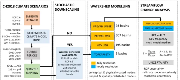
The analysis chain is shown in detail in Figure 6.1. The details of the CH2018 Climate Scenario development chain can be found in CH2018 (2018) and are not repeated here. The quantile-mapped daily climate simulations produced on a 2x2 km grid were either used as direct daily input into watershed models PREVAH and HBV Light without stochastic downscaling, or further downscaled to hourly timescales by the 2-d stochastic weather generator AWE-GEN-2D (PELEG et al., 2017; 2019) and used as input into the watershed model TOPKAPI-ETH. PREVAH and HBV Light are conceptual (semi-)distributed watershed models which have been used in climate change impact studies in Switzerland in the past, and are applied here to 195 basins (HBV Light), 93 (PREVAH UNIBE), and 307 basins (PREVAH WSL) at the daily resolution, while TOPKAPI-ETH is a physically-based fully-distributed model which was applied to three basins at the hourly resolution. More details about the individual model applications are in Section 6.3.
Annual maxima (Q) were extracted for every year of the simulations and a standard Generalized Extreme Value (GEV) flood frequency analysis was conducted to estimate the flood peaks (QR) for return periods R = 2, 5, 10, 20, 30 and 50 years. For the models without stochastic downscaling (PREVAH and HBV Light) this meant a single realisation of annual floods at the daily resolution and estimates of QR for every climate model chain from which we computed the multi-model-median (MMM) of QR values for the future (FUT) and control (REF) periods and their ratio (see Figure 6.1). For the model with stochastic downscaling (TOPKAPI-ETH) this meant multiple realisations of annual floods at the hourly resolution and estimates of QR for a reduced set of climate model chains from which we computed the multi-model and ensemble median of QR values for the future (FUT) and control (REF) periods and their ratio. The future (FUT) periods were in both cases sliding 30-year periods from the current time to end of the century (1981- 2099).
In the analysis we focussed on the signal in mean flood change at the daily scale and the spatial variability between the basins in Section 6.3, and on the stochastic and climate model uncertainty in flood change at the hourly scale for RCP 8.5 in the Thur catchment in Section 6.4.
Figure 6.1: Scheme of the climate change impact analysis on hydrological processes and floods conducted as part of the Hydro-CH2018 Project (P Molnar).
6.3. Projected flood changes
PREVAH (Modellers: Zappa, Brunner, Martius, Mülchi)
Two applications of the PREVAH model were developed by the University of Bern (PREVAH UNIBE) for 93 selected basins with gauging (here we show results for a larger selection of 106 basins), and WSL (PREVAH WSL) for 307 basins covering the whole country. The main differences between these two applications of the same hydrological model are in the way they prepare model inputs and calibrate parameters. The UNIBE setup used the climate gridded input and calibrated each basin separately against observations on even years for the period 1985-2014 with the PEST algorithm. The WSL setup used the climate station input which was gridded internally and regionalised the parameters of the model to a 500x500 m grid in a calibration process that involved 140 catchments for the period 1993-1997 (more details in BRUNNER et al. 2019). The WSL setup provides predictions for area-filling catchments in Switzerland, while the UNIBE setup provides predictions for catchments corresponding to the hydrometric stations. As a result, despite using the same hydrological model, the simulations are not identical.
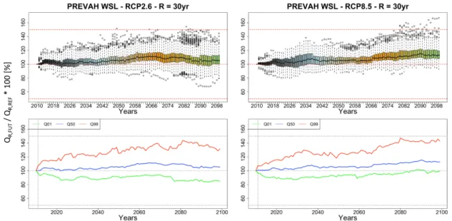
The relative change in flood peaks (FUT divided by REF in percent) for the 30-yr return period is shown in Figure 6.2 for the UNIBE setup and Figure 6.3 for the WSL setup. The box plots represent the variability between basins for 30-yr moving windows until 2099. The main messages of both model applications are as follows. First, although the median flood magnitude of all basins is slightly increasing into the future, temporal variability is large. The median increase found in both RCP 2.6 and RCP 8.5 emission scenario is only in the range of 0-10% and in fact temporal fluctuations in median change make predictions highly uncertain. In RCP 2.6 in both model applications the median change drops to almost no change by the end of the Century. Second, spatial variability between basins is large. In many catchments flood change is hardly detectable (or even negative), in others it may reach up to +50%. For example, 25-35% of the basins showed negative change in RCP 2.6, while in RCP 8.5 it was about 27% in mid Century and 2- 16% at the end of the Century. The results for floods with lower return periods are similar.
Figure 6.2: Example of simulated changes in Q30 with (left) RCP 2.6 and (right) RCP 8.5 for the PREVAH UNIBE model setup. Changes are in % of Q30 for FUT/REF in 30-yr moving windows until 2099. The boxplots (top) represent the spatial variability between catchments, the quantile
Figure 6.3: Example of simulated changes in Q30 with (left) RCP 2.6 and (right) RCP 8.5 for the PREVAH WSL model setup. Changes are in % of Q30 for FUT/REF in 30-yr moving windows until 2099. The boxplots (top) represent the spatial variability between catchments, the quantile plots (below) show the 1%, 50% and 99% percentiles. Colours indicate progression in time.
HBV UZH (Modellers: Seibert, Freudiger)
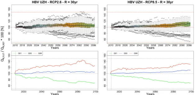
The same results are plotted for the HBV Light model calibrated and validated on 195 basins in Switzerland in Figure 6.4. The HBV application was oriented on the streamflow response in catchments with important cryosphere processes. In the calibration and regionalisation of parameters headwater catchments at high elevations were used – 190 of them with glacier cover and 5 without. Despite this difference in elevations, HBV and PREVAH models generally agree that there is large temporal variability in the median change and large spatial variability between basins. HBV results also show that in several catchments flood changes were strongly negative. Although the RCP 8.5 scenario has a slightly stronger signal than RCP 2.6, like in PREVAH, the natural temporal variability in flood change contains the no-change scenario.
The spatial distribution of changes in flood magnitudes between the catchments is shown in Figure 6.5 for all models for mid-century (2050) and end-of-century (2099).
There seems to be an indication towards stronger increases in flood peaks in the mountain catchments in PREVAH, while in HBV there are large differences between individual catchments. The strongly negative changes (orange and red) in RCP 8.5 in HBV simulations belong to the 20 most glacierized catchments (out of 195) modelled.
For example, the dark red catchment at the end of Century in southern Switzerland is at the mouth of the Gorner glacier, where simulations show a dramatic reduction in streamflow and floods due to glacier retreat. In this case, increased rainfall in a future climate is not high enough to compensate for the loss of the glacier melt contribution to discharge. Overall, spatial variability in flood change predictions is large and it is difficult to highlight spatially consistent trends at the level of individual catchments from the results reported in Figure 6.5.
QR,FUT/ QR,REF* 100 [%]
Figure 6.4: Example of simulated changes in Q30 with (left) RCP 2.6 and (right) RCP 8.5 for the HBV model. Changes are in % of Q30 for FUT/REF in 30-yr moving windows until 2099. The boxplots (top) represent the spatial variability between catchments, the quantile plots (below) show the 1%, 50% and 99% percentiles. Colours indicate progression in time.
Figure 6.5: Example of simulated changes in Q30 for all analysed basins with PREVAH UNIBE (left column), PREVAH WSL (centre) and HBV UZH (right column) for the RCP 8.5 scenario in mid-century (top row) and end-of-century (bottom row). Changes are expressed as % of the estimated Q30 for FUT/REF. Green tones indicate increases, red tones indicated decreases in flood peaks. Bright green means that the GEV fit failed in those catchments and no results are reported.
A summary table of the results for all models and two return periods is provided in Table 6.1 for all catchments as well as a subset of catchments with mean elevations above 1600 m. It can be concluded that flood peaks on the average are increasing in all modelled scenarios in the range 0-10%. However, the uncertainty is large already in the case of small return periods, the mean change is of similar magnitude to the spatial standard deviation between catchments. This becomes even more obvious for higher
QR,FUT/ QR,REF* 100 [%]
return periods. This means that although there is a clear tendency towards increases in floods, it has to be acknowledged that the rates of increases are small and the regional signal in flood change is highly uncertain.
Table 6.1: Mean change in median QR for R = 5 and 30 years with range ±1 standard deviation for three models and RCP 2.6 and RCP 8.5. Results are shown for mid-century and end-of- century for all catchments (left) and catchments with mean elevation > 1600 m (right).
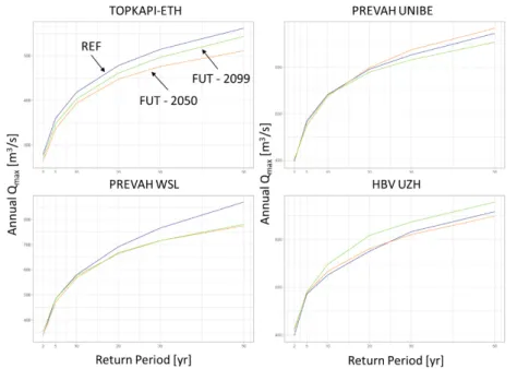
The analyses reported above have additional important limitations. First, the hydrological models have their own parameter and model uncertainty which affect performance at individual basins. This is obvious when the annual flood frequency curves for REF and FUT are shown for the individual models in the same catchment, e.g. Thur in Figure 6.6. TOPKAPI ETH and PREVAH WSL predict decreases in flood peaks in this catchment in the future, while PREVAH UNIBE and HBV UZH predict no consistent change. The models also don’t predict the annual flood observed data equally well, especially if these were not included in the calibration procedure (e.g. TOPKAPI-ETH was calibrated on hourly data). Second, the uncertainty in the GEV fitting procedure can be equally important, i.e. the confidence bounds predicted by GEV for high return periods will easily overlap for REF and FUT simulations. This is a warning that catchment specific parameterizations and hydrological model choice may be equally important for predictions and deserve detailed attention in future studies.
Figure 6.6: Example of simulated changes in flood frequency curves (daily maxima) by all four models for the RCP 8.5 emission scenario for current climate, mid-century 2049 and end-of- century 2099 at the Thur Catchment.
ALL CATCHMENTS
RCP 2.6 - R = 5yr RCP 8.5 - R = 5yr
Model Yr 2050 Yr 2099 Yr 2050 Yr 2099
PREVAH WSL 103% ± 5% 104% ± 7% 105% ± 4% 110% ± 8%
PREVAH UNIBE 104% ± 5% 101% ± 7% 104% ± 5% 106% ± 8%
HBV UZH 106% ± 7% 107% ± 10% 105% ± 7% 104% ± 13%
RCP 2.6 - R = 30yr RCP 8.5 - R = 30yr
Model Yr 2050 Yr 2099 Yr 2050 Yr 2099
PREVAH WSL 105% ± 8% 105% ± 10% 106% ± 7% 113% ± 9%
PREVAH UNIBE 105% ± 12% 104% ± 9% 104% ± 7% 108% ± 10%
HBV UZH 104% ± 8% 105% ± 11% 104% ± 6% 111% ± 13%
CATCHMENTS > 1600 m
RCP 2.6 - R = 5yr RCP 8.5 - R = 5yr
Model Yr 2050 Yr 2099 Yr 2050 Yr 2099
PREVAH WSL 105% ± 5% 111% ± 6% 105% ± 4% 114% ± 9%
PREVAH UNIBE 104% ± 5% 103% ± 8% 103% ± 4% 105% ± 9%
HBV UZH 106% ± 7% 107% ± 10% 105% ± 7% 104% ± 13%
RCP 2.6 - R = 30yr RCP 8.5 - R = 30yr
Model Yr 2050 Yr 2099 Yr 2050 Yr 2099
PREVAH WSL 104% ± 7% 105% ± 12% 104% ± 7% 119% ± 10%
PREVAH UNIBE 103% ± 7% 100% ± 10% 103% ± 6% 115% ± 11%
HBV UZH 104% ± 8% 105% ± 11% 104% ± 6% 111% ± 13%
6.4. High resolution (hourly) changes
TOPKAPI-ETH (Modellers: Moraga, Peleg, Molnar)
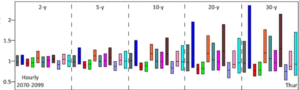
In three pre-Alpine catchments (Kleine Emme, Thur, Maggia), the physically- based watershed model Topkapi-ETH was used together with a stochastic weather generator model to make flood predictions at the hourly resolution. The weather generator simulated 10 realisations of hourly climate variables (precipitation and air temperature) for the current climate (REF) and future climate (FUT) periods for 9 climate model runs EUR-11 (see Figure 6.1). The individual climate model runs were used to quantify internal climate variability (stochastic uncertainty) in floods for each model run and the multi-model-median (MMM). The results in Figure 6.7 for the Thur Catchment are shown for all studied return periods. The TOPKAPI-ETH model predicts no change in flood peaks in the Thur for the MMM. Some climate model simulations (bars) show a decrease in future flood peaks while other show an increase. Changes in annual maximum streamflow were statistically not significant and within the range of present-day natural variability (first grey bar in figure). Internal climate variability clearly produces a large variability in flood peak estimates. Similar results were found for the Kleine Emme and Maggia catchments.
Figure 6.7: The ratio between annual maximum streamflow for a given return period of present climate (REF) and end-of-century climate (FUT 2070–2099) at the hourly scale. Bars from left to right refer to observed natural variability (grey bar), the 9 different climate models, and the multi- model mean (MMM, light blue). Box plots represent the stochastic uncertainty for each climate trajectory (model uncertainty), and for MMM they represent the combination of stochastic and climate model uncertainty. Central lines in the box plots represent the median change computed from the simulated ensemble using GEV distributions, while the boxes represent the 5–95th percentile range of the data. The simulated ensemble for each climate trajectory is composed of 30 realizations of 30 years each, bootstrapped from an archive of 100 years (N. Peleg).
Take-Home Messages
The results of Hydro-CH2018 analysis for 3 watershed models and up to 300 basins suggest a tendency towards increases in flood magnitude in Switzerland in future (in the range 0-10%) on the average. However, the changes in flood magnitudes are much less significant than the changes in the general hydrological regime due to the differences in how floods are represented in the hydrological models and the role of internal climate variability in their generation.
There is large temporal variability in flood change predicted by the climate models, temporal fluctuations in median change make predictions highly uncertain, especially for RCP 2.6.
There is large spatial variability in predicted flood changes, some catchments are very sensitive to changes in precipitation and air temperature and produce much larger floods, and in others such as the glaciated catchments the predicted flood changes are negligible or even strongly negative when ice melt contributions to runoff disappear in the future.
Including internal stochastic variability in climate forcing leads to the conclusion that changes in flood peaks, especially for very large floods, are extremely uncertain, and lie within the natural variability of floods even in the current climate.
This means that predictions of flood changes in individual catchments based on the watershed model results are still challenging.