D I V E R S I T Y A N D STA B I L I T Y I N F O O D W E B S
Impacts of Non-Equilibrium Dynamics, Topology and Variation
���������- ������������
zur
Erlangung des Doktorgrades
der Mathematisch-Naturwissenschaftlichen Fakultät der Universität zu Köln
vorgelegt von
����� �����
aus Köln
Köln, 2016
Berichterstatter: Prof. Dr. Alexander Altland
(Gutachter) Prof. Dr. Joachim Krug
Tag der mündlichen Prüfung: 11.07.2016
K U R Z Z U S A M M E N FA S S U N G
Mit fortschreitendem Klimawandel wird der Erhalt des Artenreichtums immer wichtiger. Nur bei genügend großem Genpool und breitgestreuten Bedürfnis- sen der Arten an ihre Umgebung werden sich Spezies finden, die sich verän- derten Umständen anpassen können. Um Biodiversität zu erhalten, muss aber zunächst einmal verstanden werden, welches Vorgehen welche Folgen nach sich zieht. Mathematische Modelle der Populationsdynamiken könnten ent- sprechende Prognosen liefern. Es fehlt aber noch ein Modell, das dazu in der Lage wäre, die Mechanismen, der alltäglich und experimentell beobachteten Artenvielfalt wiederzugeben und zu erklären. Eine Kombination theoretis- cher Modelle mit detaillierten Experimenten ist notwendig, um biologische Prozesse in Modellen zu testen und die Vorhersagen mit den Auswirkungen in der Wirklichkeit zu vergleichen.
In der vorliegenden Arbeit werden verschiedene Nahrungsnetze modelliert und untersucht. Unter anderem werden Modelle zu Experimenten des zo- ologischen Instituts der Universität zu Köln entwickelt und analysiert. Hier weisen Simulationen der Laborsystemen eine gute Übereinstimmung der nu- merischen Daten mit den experimentellen Ergebnissen auf. Mit Hilfe der Sim- ulationen kann gezeigt werden, dass wenige Modellannahmen nötig sind um langanhaltende Oszillationen der Populationsgrößen zu reproduzieren. Allerd- ings zeichnet sich ebenfalls ab, dass ein Zusammenleben „zufällig zusammen gewürfelter“ Arten über lange Zeiträume nicht sehr wahrscheinlich ist. Auch größere Nahrungsnetzmodelle zeigen keine signifikante Abweichung von diesen Beobachtungen und belegen wie außergewöhnlich und kompliziert die natürliche Vielfalt ist. Um eine solche Koexistenz zufällig ausgewählter Arten wie im Experiment regelmäßig zu erzeugen, müssten andere Prozesse oder weitere Einschränkungen in die Modellannahmen eingehen. Eine andere Erk- lärung für die beobachtete Koexistenz ist ein langsames Aussterben. In nu- merischen Simulationen überleben Arten vergleichbare Zeitspannen wie im Experiment bevor sie dann letzten Endes aussterben.
Interessanterweise kann festgestellt werden, dass dieselben mathematischen Modelle auch ein Überleben mehrerer Arten im Gleichgewicht erlauben und somit nicht dem sogenannten Konkurrenzausschlussprinzip folgen. Dieser Gleichgewichtszustand ist allerdings fragiler gegenüber Änderungen der Nah- rungszufuhr als die oszillierende Artenvielfalt. Insgesamt belegen die Un- tersuchungen, dass Koexistenz eher oszillierende Populationsgrößen aufweist und dass andererseits oszillierende Populationsgrößen ein Nahrungsnetz
iii
iv
sowohl gegen demographisches Rauschen wie auch gegen Änderungen des Lebensraums stabilisieren.
Diese Modellvorhersagen sind sicher nicht eins zu eins auf reale Ökosys-
teme übertragbar, aber bei der Regulierung von Tierbeständen sollte der stabil-
isierende Charakter von Fluktuationen bedacht werden.
A B ST R A C T
With progressive climate change, the preservation of biodiversity is becoming increasingly important. Only if the gene pool is large enough and requirements of species are diverse, there will be species that can adapt to the changing cir- cumstances. To maintain biodiversity, we must understand the consequences of the various strategies. Mathematical models of population dynamics could provide prognoses. However, a model that would reproduce and explain the mechanisms behind the diversity of species that we observe experimentally and in nature is still needed. A combination of theoretical models with de- tailed experiments is needed to test biological processes in models and com- pare predictions with outcomes in reality.
In this thesis, several food webs are modeled and analyzed. Among others, models are formulated of laboratory experiments performed in the Zoological Institute of the University of Cologne. Numerical data of the simulations is in good agreement with the real experimental results. Via numerical simulations it can be demonstrated that few assumptions are necessary to reproduce in a model the sustained oscillations of the population size that experiments show. However, analysis indicates that species "thrown together by chance" are not very likely to survive together over long periods. Even larger food nets do not show significantly different outcomes and prove how extraordinary and complicated natural diversity is. In order to produce such a coexistence of randomly selected species—as the experiment does—models require additional information about biological processes or restrictions on the assumptions. Another explanation for the observed coexistence is a slow extinction that takes longer than the observation time. Simulated species survive a comparable period of time before they die out eventually.
Interestingly, it can be stated that the same models allow the survival of several species in equilibrium and thus do not follow the so-called competitive exclusion principle. This state of equilibrium is more fragile, however, to changes in nutrient supply than the oscillating coexistence.
Overall, the studies show, that having a diverse system means that popula- tion numbers are probably oscillating, and on the other hand oscillating popu- lation numbers stabilize a food web both against demographic noise as well as against changes of the habitat.
Model predictions can certainly not be converted at their face value into policies for real ecosystems. But the stabilizing character of fluctuations should be considered in the regulations of animal populations.
v
C O N T E N T S
1 ������������ 1
1.1 Outline of this thesis 3
1.2 Fundamentals of ecological models 5 1.2.1 Food Web Models 6 1.2.2 Chemostat Experiments 11 1.3 Diversity in Dynamic Populations 14
1.3.1 Competitive Exclusion and Chaotic Coexistence 14 1.3.2 Stochastic Fluctuations and Demographic Noise 18 1.3.3 Verification of Chaos 18
2 ����� ����������� � ��������-���� ������ 21 2.1 Introduction 22
2.2 Methods 24
2.3 Theoretical Results 26 2.4 Discussion 33
3 ����������� �� ����������� ����� ��� ����������� 35 3.1 Introduction 36
3.2 The model by Huisman & Weissing 37 3.3 Chaotic Coexistence 38
3.3.1 The Experiment 38 3.3.2 The Model 39 3.3.3 Results 43
3.4 Equilibrium Coexistence 46 3.4.1 Results 49
3.5 Statistical Analysis 49 3.5.1 Methods 50 3.5.2 Results 50 3.6 Discussion 51
4 ��������� �� �����������, ����������� ��� ��������������
55
4.1 Introduction 56 4.2 Methods 57
4.2.1 Statistical Approach 57 4.2.2 Model 57
4.3 Results 60
vii
viii Contents
4.4 Discussion 62
5 ������ �� ������� ��������� ��� ���������� 65 5.1 Introduction 65
5.2 Methods 66 5.3 Results 70 5.4 Discussion 73 6 ������� 75
Appendices: Code
a ����� ����������� � ��������-���� ������ 81 a.1 Lyapunov Exponent 81
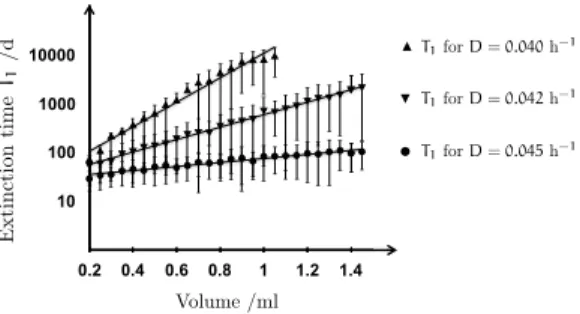
a.2 Extinction Times 83 a.3 Bifurcation Diagram 88
b ����������� �� ����������� ����� ��� ����������� 91 b.1 Model setup adapted from Huisman and Weissing 91 b.2 Parameter values for Figure 15 91
b.3 Time evolution 92 b.4 Contourplots 92
b.5 Biomass and Production 93 b.6 Largest Lyapunov Exponent 93 b.7 Statistical Analysis 94
c ��������� �� �����������, ����������� ��� �������������� 97 c.1 Model setup 97
c.2 Time evolution 98
c.3 Mapping all configurations with 20 initial species 98
d ������ �� ������� ��������� ��� ���������� 101
Bibliography 105
1 I N T R O D U C T I O N
‘The highest function of ecology is understanding consequences.’
— Frank Herbert, Dune
Earth’s biosphere is a complicated worldwide interaction network of all species. With growing human population and an increasing impact due to fishing, managing livestock and fisheries management is an ever-growing task [93]. Ecosystems suffer from the cumulative transformation of natural habitats due to direct human influence but also from climate change, droughts, temperature shifts, et cetera. These environmental variations change the composition of species in an ecosystem, influence the population numbers but more importantly, puts several species at imminent threat of extinction and whole ecosystems to collapse. Understanding population dynamics and predicting the evolution of food webs becomes more and more important.
What limits the number of species—the diversity—in a system? What is the influence of a species on the biological diversity in its habitat? How stable is the balance between the species? How severely does an ecological system react to different external influences? Questions of this type are highly relevant both from a fundamental and a social and economical point of view.
We depend on (and are part of) this system’s dynamics and development.
Exploitation of the oceans for fish, life stock management, extinction of crop pollinators et cetera have direct impact on human life. The tolerance to overfishing of fish stocks, for instance, can have major social and economical consequences. Even more so with growing population pressure and climate change. Understanding the mechanisms leading to a collapse of systems is crucial for food security. If we want to preserve biodiversity we have to know on which ground to make decisions. The question whether chaotic fluctuations occur under realistic conditions and how this will affect the stability and diversity of ecosystems is of obvious relevance.
Once the interactions between species and predator-prey-relations in a food-net are understood, theoretical models predicting its behavior can be developed. Since the classical works of Lotka [69] and Volterra [118] in the 1920s, theoretical modeling has led to important and often surprising contributions to the understanding of ecosystems. For example studies by
1
2 ������������
Leibold [61] promoted the concept of keystone predators [83]. They predict that predators play an important role in maintaining species diversity: only in the presence of a common predator more than one species can survive in a shared habitat on one trophic level. In the absence of predatory pressure one species will suppress all others.
Various theoretical works indicate deterministic chaos in food webs [42, 74, 75, 102, 103]. On the one hand chaos leads to population fluctuations which are unpredictable, even the smallest uncertainties in the initial situation cause great effects in population levels. On the other hand, and somewhat contrary to intuition, it might contribute to the stabilization of food webs. If population numbers are confined to a chaotic attractor, they are bound from above as well as from below and are thereby prevented from extinction: chaotic fluctuations notwithstanding, the ecosystem is stable in the sense that it retains its original form as a whole. This is also true for systems in which a coexistence of all species in a stable stationary state is not possible.
We cannot hope to model and simulate all species in a natural habitat in the minutest detail along with the complex web of their interactions, specific parameters and movement. To tackle this complex system there are two approaches, both with their own weaknesses and advantages. One way to go is to concentrate on a few “most important” species or to “coarse grain”
and combine species into functional groups by their hunting behavior or role in the ecosystem. The latter approach is taken for example by global models of the oceanic ecosystem [16, 120] but has also been applied successfully on smaller scale in niche models reproducing food web structures of lake systems via Monte Carlo simulations [122].
The other route to take is first to study small food webs or motifs in the interaction network [79]. This is a reasonable strategy, as we can assume, that such communities exist in isolation for some timespan till interacting with the environment. Moreover, the global development in a system certainly depends on the underlying subsets. The collective behavior of coupled dynamical systems in more complex systems is not always predictable, but some rough generalizations are known [100]. Characteristics of and results for small food webs generalize to larger webs [123] and can be interpreted as webs for functional groups. The values characterizing the behavior and growth of species are not easily all determined and vary inside natural populations. By numerically simulating hundreds of food webs with slightly different parameters we can get an idea of how likely particular configurations will develop by chance under fixed assumptions and formulate general rules regarding dynamics in communities of species.
In an analogous manner whole-ecosystem experiments will control and
observe a selection of parameters but not all. The problem with these
approaches is that species that are small in numbers can still have an important
�.� ������� �� ���� ������ 3 influence on the rest of the habitat and thus might incorrectly be overlooked as insignificant. Certain mechanisms might not be observed this way.
Our paradigm are small microbial food webs. Well controlled laboratory experiments in chemostats can provide a basis for such models. Chemostats are closed containers with microbial species in water with constant food inflow and overflow, controlled temperature and light. Such a food web in chemostat offers maximal control of the species introduced as well as the environmental parameters. Accordingly such a microbial aquatic food web is our minimal model. It makes use of well-studied growth laws and established models [14, 63], offers comparable hypothesis for experiments and is still variable enough to deal with diverse questions. To address more general aspects of the problem we increase the degree of complexity in our models: The structure of a food web can be more or less complex, species might entertain stronger or weaker interactions. The number of interdependent species in the web could alter the stability of diversity as well as the number of levels.
The aim of this study is to look for robust mechanisms that guarantee coexistence of several species and to identify classes of food webs with regard to their stability and species diversity. Those classes can for example be characterized by the topology of their inter-species relations, e.g. feeding on products of metabolism of another species or competition on nutrients or via a common predator.
�.� ������� �� ���� ������
Natural food webs manifest a complexity that fascinates and poses challenges at the same time. With few ingredients, a relatively simple and small food web of three species can exhibit various dynamical patterns from equilibrium over limit cycles to chaotic attractors (as we will see in chapter 2). Chaotic and non linear dynamical systems have been studied extensively in theoretical physics, in the realm of laser physics, mechanical vibrations or socio-economic problems. In the field of ecological models, the role of non-equilibrium dynamics is not fully understood and still in development.
The present work results from a close cooperation with experimental biol-
ogists that aimed at an understanding of maintained diversity and sustained
oscillations in real world systems. This offered unique and exciting opportu-
nities but on the other hand such a collaboration involves uncertainties: The
availability of new data and the execution of new experiments cannot be con-
trolled and novel challenges arise. Theoretical models of practical laboratory
experiments were simulated numerically to compare to empirical data and the
4 ������������
influences of species interactions 1 . With the many unknown parameters in ecology and the natural variation, random sampling of parameters and numer- ical simulations offer one way to explore dynamics and diversity of food webs without restricting the analysis to explicit parameter values.
This dissertation mainly addresses three questions:
1. Which factors affect the stability of a food web or an ecosystem?
2. How does the composition of a food web or an ecosystem affect its stability?
3. Are some species more important than others concerning food web stability?
Stability in this contexts refers to the persistence of species diversity in a sys- tem, i.e. to the stability of the number of distinct species and to the resistance to changes in the system’s parameters. A potential loss of species corresponds to an unstable system, in a stable system the number of species stays constant.
The aim is to infer system properties that indicate strong or weak stability against external perturbation. This would help deciding which species in a food web are most important to protect and which habitat could be especially prone to breakdown.
After reviewing the fundamentals of ecological models and diversity and defining the required terms in section 1.2 and 1.3, chapter 2 investigates a predator-prey model that simulates the life chemostat system of Becks et al.
[10]. In the experiment as well as in the model, chaotic population dynamics occur over broad parameter ranges. The model reproduces experimental data qualitatively with population abundances of apt orders of magnitude. The system features a chaotic attractor that arises from the interplay of two dis- tinct limit cycles. Demographic numerical simulations demonstrate that the attractor in turn causes the mean extinction times of the food web to increase exponentially with system size. In other words chaos stabilizes the populations against demographic noise.
Chapter 3 reviews a theoretical model [47] and modifies it to describe the processes in the chemostat experiment realized by Schieffer [94] and Arns [7] in Cologne. The chapter addresses the feasibility of coexistence in non- equilibrium as well as fixed population numbers. Although both types are possible in numerical simulations, chaotic coexistence proves much more sta- ble under changes of dilution rates. Not only does chaos (or fluctuations)
1 The numerical calculations here and in the following chapters were either performed with C++ or with
Mathematica Version 10 (Wolfram Research, Inc., Mathematica, Version 10.0, Champaign, IL (2014)).
�.� ������������ �� ���������� ������ 5 support multi-species coexistence but it also stabilizes diversity better against perturbations than stationary setups. On the other hand, numerical calcula- tions show that high species richness is not a likely outcome under the general assumptions of the model. Natural diversity needs additional explanations and mechanisms.
Chapter 4 examines the impact of specialization and the excretion of metabolic products on competitive microbial communities. A numerical study of systems of 20 competitors was performed. The model features a common good, excreted by producers, that can be utilized by generalists. Varying the food web structure (the number of producers and generalists) and sampling random species with fixed species interactions we draw the conclusions that first, producers enable higher species richness and second, that specialists pro- mote diversity.
Chapter 5 explores in a third model the consequences of the food web structure on stability and diversity in systems. Starting with a substantially larger number of species and multiple trophic levels, diversity still declines over ecological time scales. On average, systems end up with three to four species and four trophic levels above the resources. An investigation of dynamical properties indicates the importance of non-equilibrium dynamics for the maintenance of species richness in ecosystems.
Code for the simulations of each chapter can be found in the respective appendices.
�.� ������������ �� ���������� ������
“We remembered the relationship between a food animal called a snowshoe rabbit and a predatory cat called a lynx. The cat population always grew to follow the population of the rabbits, and then overfeeding dumped the predators into famine times and severe die-back.”
— Frank Herbert, Chapterhouse Dune
Historically, the field of population dynamics developed not so much from mathematical biology but from considerations mostly concerned with human population in particular. Malthusian growth models—named after Robert Malthus [72] and his influential essay "on the principle of population”—
assume exponential growth with a constant rate r dP
dt = rt , P(t) = P 0 e rt (1.1)
6 ������������
where t is the time and P 0 the initial population size. With positive growth rate r the population grows indefinitely, if r is negative, population numbers approach zero. Malthus assumed linear growth in food production and accordingly predicted a future of famine and starvation for British society when, in 50 years from then (1798) on, population numbers would have overtaken food supply. Luckily for Great Britain, farming became more efficient and society did not follow this simple growth model.
In 1838 Verhulst [115] published an equation incorporating the limited carrying capacity of an environment to support a population.
dP dt = rP ·
✓ 1 - P
◆
, P(t) = P 0 e rt
+ P 0 (e rt - 1) (1.2) This model predicts more realistic logistic growth where populations saturate at the maximum value lim t!1 P(t) = when resources like food or space get scarce.
During this period, theoretical ecological sciences started to evolve. Sprengel [97] and von Liebig [119] developed and promoted, respectively, an agricultural theory about plant growth and the optimal use of mineral fertilizer. They formulated a principle stating that the growth of crops is controlled by the scarcest resource.
In 1926 Volterra [117, 118] published the famous Lotka-Volterra equations to explain fluctuations in the statistics of fish catches. He also discussed potential application to plant parasites. Independently, Lotka [69] derived the same type of predator-prey equations in 1925 after proposing them for the description of autocatalytic chemical reactions in 1910. Volterra discussed basic interactions of two or three species competing for food or feeding on one another. These models predict stationary population numbers, damped oscillations or ongoing oscillations in the case of the popular predator-prey system.
Still nowadays population models are a measure to predict development of food supply and to ensure it by managing livestocks, fisheries and ecosystems in general.
�.�.� Food Web Models
In the life sciences, population dynamics study the size of populations of species or groups of species in a mutual environment.
The definition of a biological species via genetic differences or reproduction
is not always well-defined. In the theoretical framework, we will define a
species in terms of its traits. Members of one species are distinguished from
�.� ������������ �� ���������� ������ 7
Figure 1: Reconstructions of fossil food webs and trophic levels from the Chengjiang and Burgess Shale produced by Dunne et al. [22]. Species or taxa are represented by spheres, connected by feeding links. The lowest level is composed of primary producers (red), the top level contains predators (yellow). Food webs can be simplified by gathering species by common feeding behavior into "trophic species”.
S: number of species (nodes). L: number of trophic links. C: connectance; L/S2.
MaxTL: maximum trophic level of a species in the web.
http://dx.doi.org/10.1371/journal.pbio.0060102.g001
other species by properties like growth rate, the way they interact with other individuals and the environment et cetera.
In natural ecological systems, several species live together, interacting with each other. A food web represents the combined trophic (feeding) interactions graphically. Arrows indicate directed feeding links or rather who eats whom. Sometimes this is also referred to as the flow of energy or nutrients through the web. Starting at the lowest level with producers (autotrophs) like phytoplankton, algae and plants that convert light, mineral nutrients and gas into organic matter. The next higher level would be consumers grazing on the producers. These will be fed on by the next higher rank of predators and so on. In a simple case, species with mutual predators and prey or resources can be ordered into trophic levels. Inside each level several species compete against each other for food but also in defense against predation pressure. If we consider only one species per level (A eats B eats C) one might also call this a food chain. In general natural ecosystems can be much more complex and interconnected (see Figure 1).
To describe population numbers in ecological systems mathematically, we treat the number of individuals of each species as a continuous quantity.
By neglecting the discrete nature of birth and death processes we implicitly
assume sufficiently large system sizes and numbers. This assumption breaks
of course down for small systems. Consequences from the discreteness in small
systems are discussed in chapter 2. Another approximation in this study is that
the aquatic communities are well mixed and that this process destroys spatial
8 ������������
information. Seasonal environmental fluctuations will not be considered, just as age structure of the populations.
All changes in population numbers can then be incorporated into rate equations. Growth and death rates determine the evolution and might depend explicitly on the numbers of predators or the availability of nutrients or implicitly on the abundance of competitors . In these systems—homogeneous in time and space—this will result in coupled differential equations of first order that do not depend on time explicitly.
One Species
To define the main ingredients we consider the Malthusian model of a single population without external restrictions. With N we refer to the number of individuals and with t to the time. (In other contexts we might as well refer to a population density of, say, cells per liter. It can have advantages to define equations independent of the total volume.) Characterizing mortality and reproductivity by mortality rate m and birth rate µ, respectively, the rate equations are
dN
dt =bN - mN = (b - m)N = ↵N. (1.3)
Here the mortality rate specifies the ratio of the population dying in each unit time, and the birth rate the ratio of reproducing or new individuals per time.
The net per capita change per time is then the combined rate ↵ = b - m. The differential equation of first order for N is solved by an exponential
N(t) = N 0 e ↵t (1.4) Population numbers will either grow indefinitely if ↵ is positive or decline when ↵ takes values below zero.
�������� ���� �������� �������� The next step is to take into account nutrient dependence. A basic interaction of one consumer population growing on a single resource can be described by the following equations.
dR
dt =g - ✏µ(R)N dN
dt = (µ(R) - m) N
(1.5)
The concentration of resource R affects the concentration of consumers N and
vice versa. With g we denote the net growth of resource in a system without
consumers (for example production minus degradation). A mortality rate
�.� ������������ �� ���������� ������ 9
gr ow th rat e
resource ability
I
II III
Figure 2: Types of functional response according to Holling [46]
of consumers m counteracts their growth or reproduction rate µ(R). Both, mortality and growth, are described as rates per capita and time. Growth should obviously depend on the availability of food. The resource intake and consumer growth are related by the factor ✏ that describes the amount of resource needed to yield one new consumer.
����� �� ���������� �������� Obviously the system’s population dy- namics depend on how effective species process nutrients or handle prey.
Holling [46] characterized three major types of predation by their functional response (or growth rate function) µ(R). The simplest assumption (Holling’s type I) is a linear dependence on food density. Holling’s type II and III as- sume a limited ability to process resources and to reproduce and are thereby saturating to a maximal growth rate for high resource concentrations. Type II grows linearly with low resource concentration, type III (sigmoidal functional response) follows a more than linearly increasing function (see Fig. 2). Monod [80] set up an equation similar to Holling’s type II to model growth kinet- ics that were found in empirical studies on microbes in aquatic environment.
Monod’s equation or Holling’s type II is the typical choice for µ(R) in the context of bacterial and microbial growth [14, 63].
µ = µ max R
R + R (1.6)
The specific growth rate µ is bounded by a maximal growth rate µ max . When resource concentration amounts to R , organisms grow at half the maximal rate (half saturation constant).
Two Species: Predator Prey Systems
By introducing predators feeding on prey we can expand the model to multiple
trophic levels and describe more complex food webs. Simple predator prey
10
P������������
NP re d at or ab u n d an ce P Ab u n d an ce N, P
Time t
Vol = 100;
\[Alpha]2 = 1;
\[Gamma]1 = 1/Vol;
\[Gamma]2 = 1/Vol;
\[Alpha]2 = 1;
\[Gamma]1 = 1/Vol;
\[Gamma]2 = 1/Vol;
AbundanceN,P
A B
Prey abundance N
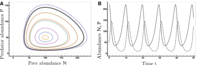
Figure 3: Simulations of a Lotka-Volterra system (1.7) with ↵
1= 0.5,↵
2= 1,
1=
2
= 0.01
left: Trajectories in phase space for several initial configurations, the gray cycle corresponds to the trajectories in the right panel
right: Numbers of predator and prey evolving over time for initial conditions (N,P) = (220,50)
models have been discussed by Volterra [118] and similar equations were independently studied by Lotka [69]. A population of predators is modeled to feed on a prey population and to multiply correspondingly. For the well- known Lotka-Volterra equations the Malthusian system is extended.
dN
dt = ↵ 1 N - 1 PN = (↵ 1 - 1 P) N dP
dt = 2 PN - ↵ 2 P = ( 2 N - ↵ 2 ) P
(1.7)
The reproduction rate of the prey species is still assumed to be linear and without predators, prey would obey the exponential growth of a single-species system (1.4). The number of predators in the system P grows with the number of prey N which in turn decreases. The rate equations feature linear functional response and predators are subject to a constant death process. In this system, there are two equilibrium states. Trivially, if both species are extinct (N = P = 0) the situation will remain this way. The other solution is a coexistence fixed point in phase space (N = ↵
22
, P = ↵
11
). If initial
conditions differ from these configurations we see trajectories evolving along
a closed orbit (limit cycle) in phase space around the second fixed point (see
Fig. 3) and initial population numbers determine the cycle the system will
follow. Population numbers oscillate with a fixed frequency around the fixed
point. Inspite of the simple equations, some biological observations agree with
this prediction, e.g. the famous field observations of lynx and snow shoe hares
�.� ������������ �� ���������� ������ 11
sampling reservoir
containing culture medium
inflow at rate .
overflow at rate . microbial
community in culture medium
D
D
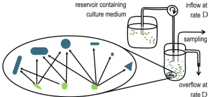
Figure 4: A schematic illustration of a chemostat experiment. Nutrient medium is pumped into a vessel containing a community of microbial organisms. This leads to an overflow from the vessel at the same rate and causes dilution in the mixture.
[24] and laboratory Paramecium-Didinium data [70]. Interestingly this particular system features a constant of motion
G = 2 N - ↵ 2 lnN + 1 P - ↵ 1 lnP (1.8) accounting for properties allowing analytical treatment. Due to its neutral pop- ulation cycles, such systems can easily be pushed to extinction by decreasing the system size and increasing stochastic noise (see e.g. Dobrinevski and Frey [21], McKane and Newman [78], Parker and Kamenev [85]). In other predator- prey systems noise can produce complex spatio-temporal structures and with long-lived population oscillations [20].
A more realistic model is the popular Rosenzweig Mac Arthur model [91]
incorporating a carrying capacity similar to Verhulst’s equation (1.2) dN
dt = rN ·
✓ 1 - N
K
◆ - NP
N + K dP
dt = NP N + K - P
(1.9)
�.�.� Chemostat Experiments
Microbial food webs are a convenient system to study population growth.
High reproduction rates allow observations of several generations during a
span of days. The system can be modified so as to model other kinds of food
webs. Communities of bacteria or phytoplankton and bacterivorous ciliates
can act as models for food webs of higher animals and vertebrates. At the
12 ������������
same time the experimental setup is transparent enough to be understood qualitatively and quantitatively. Well controlled experiments on microbial growth can be performed in a chemostat Such an installation is shown in schematic form in Figure 4. Here, an aquatic community of microorganisms—
bacteria, ciliates, algae—is cultured in a vessel in dissolved nutrients. Constant inflow from a reservoir provides nutrient medium and at the same time dilutes the system.
One Species: Consumer with Resource
As an example let us first assume a single bacterial strain and a resource and adapt equation (1.5). An important parameter characterizing this setup is the dilution rate per time, D, at which fresh medium of concentration R 0 is pumped into the vessel. This results in an effective mortality rate m = D + d where d represents the loss rate per capita from any other process as death or predation. Let us assume death rates are negligibly small in comparison to dilution. This yields the following system of equations.
dR
dt = (R 0 - R) · D - ✏µ(R) · N dN
dt = (µ(R) - D) · N
(1.10)
With this in our simple case of one bacterial consumer feeding on a resource the population of bacteria would typically grow until an equilibrium is met.
Assuming a Holling’s type II growth rate (1.6) yields the fixed point values.
dR dt = 0 dN
dt = 0 9 >
=
> ; )
D = µ(R ⇤ ) N ⇤ = R 0 - R ⇤
✏
(1.6)
)
R ⇤ = kD µ max - D N ⇤ = R 0 - R ⇤
✏
(1.11)
Obviously this result is only reasonable if nutrient concentration R ⇤ is positive, i.e. if µ max > D. This statement simply corresponds to the requirement of the maximal growth rate being greater than dilution.
This basic building block can be employed to describe competing species.
Dependance on several resources has to be included by choosing the appropri-
ate growth rates.
�.� ������������ �� ���������� ������ 13
Two Species: Predator Prey
Of course this experimental model can also be used to study predator prey systems by selecting appropriate microorganisms.The corresponding version in chemostat with Holling’s type II functional response reads
dR
dt = (R 0 - R) · D - ✏µ(R) · N dN
dt = N · (µ(R) - D) - (N) · P dP
dt = ( (N) - D) · P
(1.12)
with a newly introduced functional response of predator growth depending on the prey concentration. A loss in prey numbers accompanies the growth of predator population P. Again a conversion accounts for the number of predator organisms resulting from the loss of one prey individual.
More Species and More Resources: Competition
These models can easily be expanded to food webs of higher complexity.
Consider, for example a community of n planktonic species grazing on k resources. Population abundances N i grow depending on the availability of the resources. The availability of a resource j on the other hand, R j , depends on the consumption of resources by the plankton.
dN i
dt =N i (µ i (R 1 , . . . R k ) - m i ) i = 1, . . . n dR j
dt =D(S j - R j ) - X n i=1
c ij N i µ i (R 1 , . . . R k ) j = 1, . . . k
(1.13)
Specific mortality and growth rates are denoted by m i and µ i (R 1 , . . . R k ) respectively. A constant turnover rate D supplies fresh resources from a reservoir with concentration S j of resource j. The content of resource j in species i amounts to c ji .
Now we are faced with a new concept: The growth rates µ i (R 1 , . . . R k )
are determined by several nutrients and further considerations are necessary
to decide on the functional response. Assume that we know how a species will
respond to a single nutrient R j (provided all else is sufficiently supplied). For
microorganisms we will describe this by a function µ i (R j ) of the Holling’s
type II . Is there a way to combine the nutrient-specific growth-rates µ i (R j )
into a general growth-rate-function dependent on all nutrients µ i (R 1 , . . . R k )?
14 ������������
This will depend on the way how the nutrients are utilized by the organisms.
Nutrients can act as heterologous (=essential) in an organism. Perfectly essential means that for the species considered no resource can be replaced by any one or more of the other resources. Other chemicals might be replaceable (homologous) because they fulfill similar functions or can be converted into one another [62, 126].
For example; Huisman and Weissing [47–49] simulate a system of an aquatic phytoplankton with perfectly essential resources. We will discuss this particular case in more detail later.
�.� ��������� �� ������� �����������
For the conservation of biodiversity, we have to identify mechanisms maintain- ing and promoting species richness in natural habitats. Mathematical models can predict consequences of management strategies. The term diversity can re- fer to different quantities depending on context and author. Sometimes species abundances—the number of individuals per species— and their evenness are included and scientists calculate a weighted average. In this thesis, species rich- ness and species diversity both, will be synonymous to the number of species in a system independent of the individual population numbers.
�.�.� Competitive Exclusion and Chaotic Coexistence
Several resources limit the growth of organisms in nature: Mineral nutrients, gas, light and water are essential for survival and production. In the 19th century Sprengel [97] developed the nowadays so called Liebig’s law of the minimum. The idea was promoted lateron by Justus von Liebig[119].
"(. . . ) denn fest steht der Satz: eine Pflanze, die 9 oder 10 Stoffe zur Nahrung bedarf, kann niemals ihre höchste Ausbildung erreichen, sobald von einem einzigen dieser Stoffe nicht die erforderliche Menge vorhanden ist." — Sprengel [97]
This concept was based on the knowledge from agricultural science, that plants depend on a number of nutrients to grow. It states, that plants will grow not according to the total amount of resources, but that they are limited by the nutrient shortest in supply—the limiting factor. In other words some nutrients cannot be replaced and oversupply of one nutrient can not make up for the shortage of another.
Now consider several species limited by a number of resource. The
Competitive Exclusion Principle was formulated in 1904 by Grinnell [36] for
such systems relying on field observations.
�.� ��������� �� ������� ����������� 15
"Two species of approximately the same food habits are not likely to remain long evenly balanced in numbers in the same region.
One will crowd out the other" — Grinnell [36]
Gause [29] elaborated this idea based on laboratory experiments with two Paramecium species. He let the two species evolve in a constant environment providing a constant flow of food and fresh water. His claim was, that with constant ecological and environmental factors two species cannot compete for the same resource and coexist. He could show however, that the two species could coexist when he varied the supply of food and water. A more general formulation is that two species cannot inhabit an identical ecological niche at the same time: In a constant environment one will always outgrow the other.
This principle entails discussions about the Paradox of the Plankton:
“The problem that is presented by the phytoplankton is essentially how it is possible for a number of species to coexist in a relatively isotropic or unstructured environment all competing for the same sorts of materials.” — Hutchinson [50]
While Gause could demonstrate the principle to hold true in laboratory with two species of Paramecium or yeast, everyday experience as well as data from microcosm and mesocosm experiments show different results. Soil bacterial communities competing for a few easily digestible nutrients exhibit a high diversity [25]. Although phytoplankton growth is assumed to be limited only by nitrate, phosphate, light and carbon (because all other elements are abundant in natural waters), several thousand species can be observed in the surface layers of the world’s oceans in a relatively constant environment and little spatial structure [18, 101]. In the group of Benincà et al. [12] containers with 90 liters of water, along with sediment, detritus and the microscopic life therein were isolated from the Baltic sea. The interactions of bacteria, phytoplankton, herbivorous and predatory zooplankton and detritivores were studied over eight years in their complex aquatic habitat. Contrary to the predictions of the Competitive Exclusion Principle, the number of surviving species exceeded the number of assumedly essential nutrients (phosphor, nitrogen, carbon, light) by far.
Candidates to resolve the Paradox include chaotic advection in hydrody- namical flows, external perturbation as an ever-changing environment, spatial variation and migration. But those hypothesis cannot provide explanations for the observed coexistence in well-controlled laboratory conditions and well mixed chemostats [7, 94].
At first, theoreticians supported the Competitive Exclusion Principle by
mathematical proofs. These proofs, however, relied on linear growth rates
16 ������������
functions and searched for coexistence at stationary densities [64, 66, 71, 89, 118]. Later it has been demonstrated under more general assumptions that at fixed densities a coexistence of n species on k < n resources is impossible [77]. Nevertheless if one considers models with nonlinear growth rates and non equilibrium dynamics, coexistence of n species on k < n resources actually becomes feasible [3, 4, 54, 58, 77, 125]. Koch [58] gave numerical indication via simulations of 2-species coexistence on one resource on a periodic orbit.
Analytically this coexistence was proven for two species by McGehee and Armstrong [77]. A proof for n species coexisting on one resource was provided by Zicarelli [125] and expanded by Kaplan and Yorke [54] to more limiting factors. Gross et al. [38] proved the existence of chaotic parameter regions generically in food chains of length greater than three.
Altogether this suggests one way out of the Paradox. Namely, that a con- stant environment is not a sufficient condition for competitive exclusion, but that non-stationary population numbers make coexistence possible. The princi- ple cannot be generalized to dynamical systems and one should consider non equilibrium dynamics to account for diversity. Theoretically, non equilibrium systems may allow communities with more species than limiting resources to coexist. These dynamics are bounded and can either evolve towards a periodic limit cycle or they can be chaotic and follow a chaotic attractor, i.e. a lower dimensional complex structure embedded in the phase space of population numbers. To feature bounded chaotic solutions, autonomous differential equa- tions of first order of continuous functions have to be at least three dimensional according to the Poincare-Bendixson theorem [98]. So when the system’s di- mension exceeds three, population dynamics can become more complex and even chaotic.
This leaves the question whether biological systems commonly undergo chaotic dynamics. Or whether this explanation for biodiversity and the Paradox of Plankton is merely academic.
Experiments have shown hints of sustained oscillations in short time series of small laboratory food webs [23, 27, 53, 110]. In cultures of cannibalizing developmental stages of the flour beetle Tribolium, the mortality was changed artificially to observe crossovers from stable fixed points to chaos that had been predicted theoretically[17, 19, 44, 56]. Graham et al. [35] cultivated a community of nitrifying bacteria and protozoa in wastewater bioreactors for 207 days reporting strongly fluctuating population numbers.
Too short observation times and slow transient behavior could be a reason
that exclusion does not take place during the experiments. But in the before
mentioned long term experiment by Benincà et al. [12] species abundances
of ten aquatic functional groups and the detritus pool were counted twice a
week and the nutrient concentration was measured. This resulted in a total of
�.� ��������� �� ������� ����������� 17 690 data points per functional group, demonstrating strong erratic fluctuations in the population numbers. The duration of this experiment and sustained species richness and oscillations are a clear sign that no ’slow exclusion’ is tak- ing place. The study by Benincà et al. [12] reported that the forecast period was limited to 15 to 30 days which might indicate deterministic chaos. However, this impressive study is not without shortcomings. By gathering species into functional groups single-species information are lost. Measuring twice a week might disguise important dynamics and a lack of an external control parame- ter prevents a clear decision.
A combination of experimental results and model calculations can provide more confidence and an understanding of underlying mechanisms. Bifurcation analyses numerically confirmed chaotic dynamics for biologically relevant parameter values in models of two-prey-one-predator food webs in microbial chemostat systems [59, 114]. An actual microbial food web of this structure was examined by Becks and Arndt [8, 9], Becks et al. [10]. Bacterial strains – Pedobacter and Brevundimonas – have been placed in diluted nutrient medium together with a ciliate preying upon both. An externally controlled dilution rate determines the nutrient supply for the bacteria and at the same time acts as an effective mortality rate via overflow. And indeed by altering this parameter the population dynamics could clearly be tuned from equilibrium to periodic orbits to chaos and back in time series of 30 - 60 days duration.
Numerical simulations of plankton systems demonstrate longterm coexis- tence for particular parameter configurations as well.
Huisman and Weissing [47] demonstrated via numerical simulations of equa- tions (1.13), that for perfectly essential resources, non-equilibrium dynamics with more species than resources are possible. In the model multiple phyto- plankton species survive on a few abiotic resources in a constant environment.
Population numbers of all species can show strong sustained oscillations de- pendent on the parameter values. Huisman and Weissing provide specific parameter configurations that enabled oscillating coexistence of six species on three resources and chaotic resilience of twelve species on five nutrients. De- terministic chaos was indicated by bifurcation analyses.
It is still not clear, however, whether this specific numerical model should be treated as an exception and oddity or whether it reflects processes in real biological systems. An experiment testing this prediction was performed at the Institute for General Ecology at the University of Cologne by Schieffer [94]
and Arns [7] that will be presented and modeled theoretically in this thesis. In
the experiment up to six bacterial strains were cultivated in a common nutrient
medium containing three essential resources. The choice of bacteria was just
influenced by their ability to feed on a certain nutrient medium. Over the
18 ������������
period of the experiment (30 - 50 days) all strains survived with fluctuating population numbers supporting the thesis of chaotic coexistence.
�.�.� Stochastic Fluctuations and Demographic Noise
Ecological systems are subject to ‘intrinsic’ and ‘extrinsic’ noise sources.
Extrinsic noise could for instance be changes in temperature, fluctuations in nutrient supply and migration from external habitats. Intrinsic noise – also called demographic noise – is caused by the discrete unit steps at which population sizes change and take place even in perfectly isolated systems. Even if differential equations predict infinite survival, with demographic noise a population might die out. In the simplest case the discrete system population numbers have to take values of zero or one when the continuous system takes real number in between. Another case where discreteness can induce significant differences is a stationary coexistence in the deterministic equations.
If the continuous approximation abundances evolve towards a non-integer stable fixed point, discontinuity forces the numbers to jump "too far". The fixed point cannot be realized. Now the numbers have again to evolve back towards the fixed point. For this reason the discrete system is forced to fluctuate around the stable point. Those fluctuations may transfigure otherwise regular dynamics to behave randomly or induce periodicity [30, 109]. Such a type of effective randomness is particularly important for systems with small population sizes. Nevertheless, even in very large systems demographic noise can cause qualitative and strong effects [78]. For the food webs under consideration, the main question is how demographic noise will interfere with deterministic chaotic fluctuations present and influence stability. The discrete nature of the food-web’s dynamics is captured in the master equations of the system. These can be simulated and analyzed numerically in terms of the so-called Gillespie algorithm [31, 32]. From these simulations one can extract extinction rates in different dynamic regimes as will be done in chapter 2.
�.�.� Verification of Chaos
There are numerous ways to demonstrate chaos in dynamical systems. Prin-
cipal approaches include bifurcation diagrams, the identification of Lyapunov
exponents, or the analysis of Poincaré sections. Detecting deterministic chaos
in experiments is more difficult. Populations are always subject to intrinsic
demographic fluctuations, at levels which depend on the size of the popula-
tion and the underlying deterministic dynamics. One needs to exclude these
mechanisms, rather than deterministic chaos, as a primary cause of fluctua-
tions in the system. In the majority of cases the series of data are too short to
�.� ��������� �� ������� ����������� 19
construct bifurcation diagrams or to reliably estimate Lyapunov exponents. A
better approach is to search for parameter-dependent controllable crossovers
from stationary to chaotic behavior. In this way, chaotic and stochastic fluctu-
ations, respectively can be discriminated from each other. Model calculations
can give confirmation if experimental data demonstrates qualitative changes in
time-series.
2 C H A O S STA B I L I Z I N G A P R E DATO R - P R E Y SYST E M
Surprise? Who’s talking about surprise? Chaos is no surprise. It has predictable characteristics. For one thing, it carries away order and strengthens the forces at the extremes.
— Frank Herbert, Dune
sampling reservoir
containing culture medium
inflow at rate D
overflow at rate D
N 1
P
C N 2
P
P N 1 N 2
C C N 1 N 2
P
P N 1 N 2
C C N 1 N 2
P D
D
Figure 5: A predator P feeds on two prey species N
1,2competing for a mutual food source C. Bold arrows represent stronger energy flow, indirect influence via competition is depicted by a dashed link.
We examine a mathematical model of a simple food web consisting of two prey populations competing for nutrients and one predator population. In this model a control parameter triggers a bifurcation that initiates a transition to chaos. Chaos might alter the evolution of a system unpredictable during little time and induce wild fluctuations. Still, with the evolution of a chaotic attractor it can stabilize the system by bounding the population numbers in a region in phase space.
The experimental analogue is an aquatic system in a chemostat where similar dynamics where shown by Becks et al. [10] in Cologne. In nature such an ecosystem is exposed to different perturbations like seasonal fluctuations and stochasticity - meaning demographic noise. Interactions of the Lotka- Volterra type can easily be pushed to extinction by demographic noise [84].
In our cooperation with the group of Hartmut Arndt 1 , we aimed at finding a general catalogue of techniques to approach such a system and to analyze
1 Zoological Institute, University of Cologne
21
22 ����� ����������� � ��������-���� ������
its features. We address the question, how stable an attractor is when encountering perturbations, we characterize the stability of a chaotic attractor and we ask whether a food web will persist if ruled by deterministic chaos rather than by regular limit cycles or Lotka-Volterra-like dynamics.
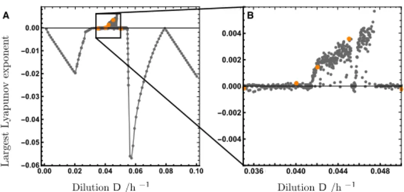
Parts of the following chapter are borrowed from [37] 2 . For a first characterization of the dynamics in this model I fall back upon parts of my diploma thesis. Starting from there, I expose the implications for generic ecological food webs, identify the deterministic chaos via the largest Lyapunov exponent and I calculate the mean extinction times of the food web numerically for the subsequent interpretation 3 .
�.� ������������
Ecological networks can show various different dynamics. As experiments confirmed they can also be ruled by deterministic chaos [10, 12, 17]. In that case the abundances of the species are restricted to a chaotic attractor undergoing large fluctuations but secure from extinction. To understand the effect of chaotic dynamics in ecological systems one can resort to a model of a small predator-prey-system. Our paradigm is an aquatic microbial community comprising two prey and a predator species. The three microscopic species are cultivated in a solution of nutrients in water in a chemostat (Fig. 7). They are constantly provided with fresh water and food.
Two bacterial strains (in experiments Brevundimonas, Pedobacter) compete for food. A ciliate (Tetrahymena pyriformis) acts as common predator. A more (less) efficient usage of food and being more (less) preferred by the predator can balance each other out and lead to a coexistence of the two strains (Fig.
6). Starting at the upmost position with many predators we can imagine the following cycle: First the less preferred species can take advantage of that fact and will grow. At the same time the number of predators decreases when the preferential food is getting sparse. With the now reduced feeding pressure the fast growing competitor will flourish. And finally the predator can reproduce again and we end up at our initial condition.
Experiments on this community have shown equilibrium, periodic and chaotic oscillations of population numbers [10]. The type of dynamics depends on the inflow of dissolved nutrients into the chemostat. This inflow—or dilution—drives the systems dynamics and acts as control parameter.
A minimal model was formulated considering the grazing of bacteria and the predation of the ciliate. The rate equations are assumed to follow ordinary
2 I have performed the numerical simulations and the analysis, created the graphics and composed the manuscript.
3 For numerical implementation see Appendix A
�.� ������������ 23
Figure 6: A predator feeds on two prey species. It prefers the prey that is faster growing.
This compensation enables the depicted cycle. In the experiment this is realized by the bacterivorous ciliate Tetrahymena pyriformis (gray) and two strains of bacteria - preferred fast growing Pedobacter (depicted by spheres) and slow growing Brevundimonas (rod like).
Holling’s type II growth. With inserting the experimentally determined specific parameters the model outcome is indeed qualitatively consistent with the experimental results.
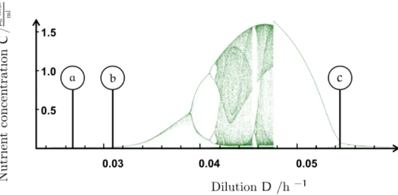
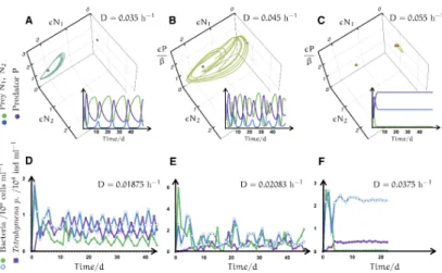
Numerical simulations of the different species concentrations undergo periodic oscillations or stay constant in an equilibrium, a regime of chaotic population dynamics is formed over a wide range of intermediate dilution strengths. This parameter window is bounded by two regimes of periodic coexistence (stable limit cycles). Chaotic trajectories stick to a structure (chaotic attractor) in phase space that seems to interpolate between the two distinct periodic dynamics. With this attractor stable coexistence of all three species is possible. An additional stability against perturbations is provided in the sense, that species abundances might react with huge fluctuations but settle quickly back onto the attractor manifold. The food web in its structure and composition remains unchanged. The same mechanism helps to stabilize against the destabilizing effects of migration and supports persistence.
In small systems finite numbers and discrete birth and death processes
produce fluctuations (demographic noise) and can push species towards
extinction that would persist in larger systems. In Lotka-Volterra systems the
mean time to extinction grows polynomially with population size[84, 85]. In
this chaotic system we can confirm the attractor’s protective properties: The
mean time to extinction in this case scales exponentially with system size.
24 ����� ����������� � ��������-���� ������
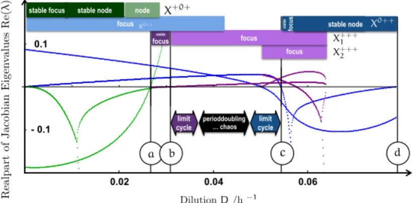
This study discusses and quantitatively models the conceptual mechanisms promoting chaotic multi-species coexistence in a two-prey one-predator model system motivated by the experiment of Becks et al. [10]. As previous studies suggest [28, 60, 103, 114] the system shows periodic and chaotic coexistence. An attractor evolves that topologically bears resemblance to Gilpin’s classification of Vance’s model [34, 57, 113]. The principles behind the formation of the attractor manifold may be summarized as follows: our system is governed by an important control parameter—the external dilution rate which acts as a paradigm for the availability of resources that the species consume. Both in the regime of low and high resource availability, the system builds up limit cycles controlling the population size. The two cycles at high and low dilution rate are topologically distinct, in a manner to be discussed below. The wide range of intermediate parameter strength is governed by a ‘competition’ between the two cycle regimes, and this will be shown to lead to the formation of a chaotic attractor interpolating between the limiting dynamics.
The suggestion that chaotic attractors may emerge from the competition between parametrically separated limit cycles is one main result of the present chapter. Fixed points and limit cycles for different parameter regimes are a generic feature of predator-prey systems and their interplay might suggest a generic mechanism promoting the transition to chaos. Below, the predictions derived for our current specific model will be shown to be in good agreement with the experiment Becks et al. [10] where population numbers in chemostat experiments could be tuned from stationary to periodic or chaotic and back depending on the applied dilution rate.
Another outcome is the confirmation of the protecting properties of chaos.
Although fluctuations strongly suppress population numbers the chaotic attractor actually protects them exponentially against extinction.
�.� �������
The system we consider models an aquatic well-mixed microbial community established in a chemostat. Prey populations compete with each other for nutrients but also via a common predator.
In the experiments under consideration two bacterial strains live on soluble
organic matter, while a bacterivorous ciliate feeds upon the two different
bacterial strains. The competition is characterized by a trade-off: one bacterial
strain is preferred by the predator but grows faster. The other strain is less-
preferred but slow-growing. At a rate D fresh nutrient solution flows into the
chemostat vessel of constant volume. Via the overflow, a mixture of microbes
and nutrients leaves the system and thereby dilutes the community inside the
�.� ������� 25
sampling reservoir
containing culture medium
inflow at rate D
overflow at rate D
N 1
P
C N 2
PP N 1 N 2
C C N 1 N 2
P
P N 1 N 2
C C N 1 N 2
P D
D
Figure 7: Outline of the experimental setup. Inset the schematic structure of interactions in the the predator prey system. Bold (thin) arrows mark strong (weak) ener- gy/biomass flow, indirect competition is shown as dashed arrow. P=predator, C=carbon source, N
1=prey 1, N
2=prey 2
chemostat. By tuning this dilution or turnover rate we will test the behavioral range of the system (Fig. 7). The following differential equations describe the temporal behavior of the concentrations in the system in the way proposed in Bohannan and Lenski [14] and Levin [64].
dC
dt =(C 0 - C)D - ✏ 1 N 1 µ 1 (C) - ✏ 2 N 2 µ 2 (C) dN i
dt =N i µ i (C) - P i (N i ) - DN i , i = 1, 2 dP
dt = 1 P 1 (N 1 ) + 2 P 2 (N 2 ) - DP
(2.1)
The concentration P of predators per unit volume grows at a per capita rate that depends on the prey populations; the concentration of prey N i declines accordingly. The grazing rate of a predator on the bacteria i is denoted by
i (N i ). The ratio of new predators per ingested prey i is i (yield). In almost the same manner the bacteria of type i multiply by a rate µ i (C) while feeding with a rate ✏ i µ i (C), where ✏ i is the reciprocal yield of ingested biomass per new prey. The growth rate µ i (C) of prey i saturates at ˆ µ i following Holling’s type II or Monod’s equation (1.6) with half saturation rate K si just as the grazing rates i (N i ):
µ i (C) = µ ˆ i C K si + C
i (N i ) = ˆ i N i
K Ni + N i
(2.2)
26 ����� ����������� � ��������-���� ������
For one specific microbial community and nutrient solution the dilution rate is the only variable left. All other parameters define biological properties of the species. The parameter values are chosen to model the specific experiments determined by Becks et al. [10] and Nomdedeu et al. [82] (see Table 1).
�.� ����������� �������
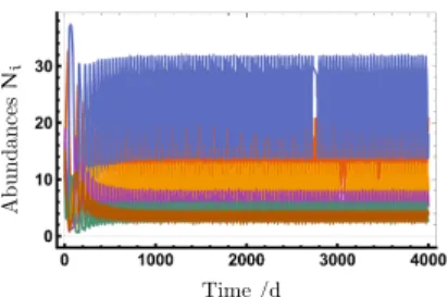
Numerical integration of Eq. 2.1 shows that the population numbers perform dynamical patterns depending on the strength of dilution. They can be organized into a few general groups: stationary, periodic and chaotic dynamics.
Without predator only one prey species will survive, the other will quickly go extinct while in the presence of a predator two species coexist. More interestingly, all three species can coexist. The dilution values corresponding to qualitative changes in the dynamics are summarized in Table 1.
Table 1: Model parameters measured in experiments by Becks et al. [10] and Nomdedeu et al. [82] and critical dilution values (numerical results up to 4 digits)
������ ���������� �����
C 0 concentration in nutrient medium [ µg Gluc ml ] 3
✏ i reciprocal yields [ µg Gluc ind
i] 2 · 10 -6 predator yields [ ind ind
pi

![Table 1: Model parameters measured in experiments by Becks et al. [10] and Nomdedeu et al](https://thumb-eu.123doks.com/thumbv2/1library_info/3705609.1506162/34.629.142.545.383.730/table-model-parameters-measured-experiments-becks-et-nomdedeu.webp)