EUROPEAN ORGANISATION FOR NUCLEAR RESEARCH (CERN)
Submitted to: Computing and Software for Big Science
CERN-EP-2021-007 19th February 2021
Emulating the impact of additional proton–proton interactions in the ATLAS simulation by
presampling sets of inelastic Monte Carlo events
The ATLAS Collaboration
The accurate simulation of additional interactions at the ATLAS experiment for the analysis of proton–proton collisions delivered by the Large Hadron Collider presents a significant challenge to the computing resources. During the LHC Run 2 (2015–2018) there were up to 70 inelastic interactions per bunch crossing, which need to be accounted for in Monte Carlo (MC) production. In this document, a new method to account for these additional interactions in the simulation chain is described. Instead of sampling the inelastic interactions and adding their energy deposits to a hard-scatter interaction one-by-one, the inelastic interactions are presampled, independent of the hard scatter, and stored as combined events. Consequently, for each hard-scatter interaction only one such presampled event needs to be added as part of the simulation chain. For the Run 2 simulation chain, with an average of 35 interactions per bunch crossing, this new method provides a substantial reduction in MC production CPU needs of around 20%, while reproducing the properties of the reconstructed quantities relevant for physics analyses with good accuracy.
©2021 CERN for the benefit of the ATLAS Collaboration.
Reproduction of this article or parts of it is allowed as specified in the CC-BY-4.0 license.
arXiv:2102.09495v1 [hep-ex] 18 Feb 2021
Contents
1 Introduction 2
2 ATLAS detector 4
3 Overview of simulation chain 6
4 Computing performance comparison 8
5 Inner detector 12
5.1 Detector readout 12
5.2 Overlay procedure 13
5.3 Validation results 14
6 Calorimeters 18
6.1 Detector readout 18
6.2 Overlay procedure 18
6.3 Validation results 19
7 Muon spectrometer 19
7.1 Detector readout and overlay procedure 21
7.2 Validation results 22
8 Trigger 22
8.1 L1 calorimeter trigger simulation 24
8.2 HLT simulation and performance 24
9 Conclusions 28
1 Introduction
The excellent performance of the Large Hadron Collider (LHC) creates a challenging environment for the ATLAS and CMS experiments. In addition to the hard-scatter proton–proton (𝑝 𝑝) interaction which is of interest for a given physics analysis, a large number of inelastic proton–proton collisions occur simultaneously. These are collectively known as pile-up. The mean number of these inelastic 𝑝 𝑝 interactions per bunch crossing,𝜇, also known as the pile-up parameter, characterises the instantaneous luminosity at any given time1.
For physics analyses, pile-up is conceptually similar to a noise contribution that needs to be accounted for. Since nearly all analyses rely on Monte Carlo (MC) simulation to predict the detector response to the physics process, it is crucial that the pile-up is modelled correctly as part of that simulation. The goal of the ATLAS MC simulation chain is to accurately reproduce the pile-up such that it can be accounted for in physics analyses.
1Hereafter, the approximation that𝜇is the same for all colliding bunch pairs is made.
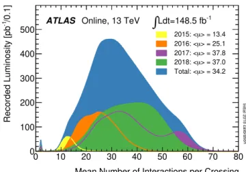
Within ATLAS, the pile-up is emulated by overlaying soft inelastic 𝑝 𝑝 interactions, in the following called minimum-bias interactions, generated with an MC generator, normally Pythia [1], according to the pile-up profile for a given data-taking period. Figure1shows the𝜇distribution for each year during Run 2 (2015–2018) and the sum of all years. The mean value is 34.2 but the distribution is broad and generally covers values between 10 and 70. The small peak at𝜇∼2 arises from special running periods with rather low luminosity. At the High Luminosity LHC (HL-LHC)𝜇is expected to increase to about 200 [2].
0 10 20 30 40 50 60 70 80
Mean Number of Interactions per Crossing 0
100 200 300 400 500 /0.1]-1Recorded Luminosity [pb
Online, 13 TeV
ATLAS
∫
Ldt=148.5 fb-1> = 13.4 2015: <µ
> = 25.1 2016: <µ
> = 37.8 2017: <µ
> = 37.0 2018: <µ
> = 34.2 Total: <µ
Initial 2018 calibration
Figure 1: The𝜇distribution observed for the ATLAS Run 2 data, for each year (2015–2018) separately and for the sum of all years [3].
The simulation chain for MC events contains several steps, starting from the generation of the interactions with an MC generator (e.g. Pythia, Sherpa [4]). The interactions of the generated particles with the ATLAS detector are simulated using a Geant4-based [5] simulation framework [6]. This is performed separately for the hard-scatter interactions of interest and a large number of minimum-bias interactions.
Next, the readout of the detector is emulated via a process known asdigitisation, which takes into account both the hard-scatter and any overlapping minimum-bias interactions. In this article, two methods of performing the digitisation are compared. The goal of the new method, described below, is to reduce the computing resources required by creating a large set of pile-up events only once for an MC production campaign and then reusing these events for different hard-scatter events.
In the first method, referred to asstandard pile-uphereafter, the hard-scatter interaction and the desired number of minimum-bias interactions are read in simultaneously during the digitisation step and the energy deposits made by particles are added for each detector element. Then the detector readout is emulated to convert these into digital signals, which are finally used in the event reconstruction. This method creates the pile-up on demand for each hard-scatter event, and has been used up to now for all ATLAS publications based on𝑝 𝑝collisions. In the second (and new) method, referred to aspresampled pile-up hereafter, this same procedure is followed but for the set of minimum-bias interactions alone, without the hard-scatter interaction. The resulting presampled events are written out and stored. Then, during the digitisation of a given hard-scatter interaction, a single presampled event is picked and its signal added to that of the hard-scatter interaction for each readout channel. This combined event is then input to the event reconstruction. In contrast to the first method, the same presampled pile-up event can be used for several hard-scatter interactions. For both methods, the𝜇value to be used is sampled randomly from the data𝜇 distribution, such that the ensemble of many events follows the𝜇distribution of the data.
If the detector signals were read out without any information loss, the two methods would give identical results. However, in reality some information loss occurs due to readout thresholds applied or custom compression algorithms designed to reduce the data volume. This can lead to differences in the reconstructed quantities used in physics analyses. While in most cases for ATLAS these differences were found to be negligible, in some cases corrections were derived to reduce the impact on physics analyses, as is discussed in Sections5–8.
Within the ATLAS Collaboration, a significant validation effort took place to ensure that this presampled pile-up simulation chain reproduces the results from the standard pile-up simulation chain accurately, so that there is no impact on physics analyses whether one or the other is used. To this end, thousands of distributions were compared between the presampled and standard pile-up simulation chains. In this article, a representative subset of relevant distributions is shown. Only comparisons between the two methods are shown in this article; detailed comparisons of data with simulation can be found in various performance papers, see e.g. Refs. [7–12].
The motivation for using the presampled pile-up simulation chain in the future is that it uses significantly less CPU time than the standard pile-up simulation chain. As is discussed in Ref. [13], savings in CPU, memory and disk space requirements are pivotal for the future running of the ATLAS experiment. Additionally, the presampled pile-up simulation chain can also be seen as a step towards using minimum-bias data, instead of presampled simulated events, for emulating the pile-up, which could potentially improve the accuracy of the modelling of the pile-up interactions. However, the pile-up emulation with data is not yet validated and not the subject of this article.
The article is organised as follows. A description of the ATLAS detector is given in Section2, highlighting the aspects that are most relevant for the pile-up emulation. Section3describes both the standard and presampled pile-up simulation chain, and Section4compares their CPU and memory performances. In Sections5–8the challenges in the inner detector, calorimeters, muon system and trigger are described and comparisons of the impact of the old and new methods are shown.
For all studies presented in this article, unless otherwise stated, the distribution of the average number of events per bunch crossing follows the distribution observed in the ATLAS data in 2017, with an average𝜇 value of 37.8 (see Figure1). The ATLAS detector configuration corresponds to that of Run 2. As the detector configuration evolves in the future, the new presampled pile-up method will need to be validated for those new detector elements.
2 ATLAS detector
The ATLAS detector [14] at the LHC covers nearly the entire solid angle around the collision point. It consists of an inner tracking detector surrounded by a thin superconducting solenoid, electromagnetic and hadronic calorimeters, and a muon spectrometer incorporating three large superconducting toroidal magnets. A two-level trigger system is used to select interesting events [15]. The first-level (L1) trigger is implemented in hardware and uses a subset of detector information to reduce the event rate from 40 MHz to 100 kHz. This is followed by a software-based high-level trigger (HLT) which reduces the event rate to an average of 1 kHz.
At the LHC, typically 2400 bunches from each of the two proton beams cross each other at the ATLAS interaction point per beam revolution, with one bunch crossing (BC) taking place every 25 ns. In each BC
several𝑝 𝑝 interactions may occur. Whenever an L1 trigger signal is received for a given BC the entire detector is read out and processed in the HLT to decide whether the event is stored for further analysis.
The inner detector (ID) is immersed in a 2 T axial magnetic field and provides charged-particle tracking in the pseudorapidity2range|𝜂| <2.5. The high-granularity silicon pixel detector (Pixel), including an insertable B-layer (IBL) [16,17] added in 2014 as a new innermost layer, covers the vertex region and typically provides four measurements per track, the first hit normally being in the innermost layer. It is followed by the silicon microstrip tracker (SCT) which usually provides four two-dimensional measurement points per track. These silicon detectors are complemented by a straw tracker (transition radiation tracker, TRT), which enables radially extended track reconstruction with an average of∼30 hits per track up to
|𝜂| =2.0. Additionally, the transition radiation capability provides separation power between electrons and charged pions.
The calorimeter system covers the pseudorapidity range |𝜂| < 4.9. Within the region |𝜂| < 3.2, electromagnetic (EM) calorimetry is provided by barrel (EMB) and endcap (EMEC) high-granularity lead/liquid-argon (LAr) electromagnetic calorimeters, with an additional thin LAr presampler covering
|𝜂| < 1.8 to correct for energy loss in material upstream of the calorimeters. Hadronic calorimetry is provided by the steel/scintillator-tile (Tile) calorimeter, segmented into three barrel structures within
|𝜂| < 1.7, and two copper/LAr hadronic endcap calorimeters (HEC). The solid angle coverage is completed with forward copper/LAr and tungsten/LAr calorimeter (FCAL) modules optimised for electromagnetic and hadronic measurements, respectively.
The muon spectrometer (MS) comprises separate trigger and high-precision tracking chambers measuring the deflection of muons in a toroidal magnetic field generated by the superconducting air-core magnets. The field integral of the toroids ranges between 2.0 and 6.0 T m across most of the detector. A set of precision chambers covers the region|𝜂| <2.7 with three stations of monitored drift tubes (MDTs), complemented by cathode strip chambers (CSCs) in the forward region, where the background is highest. The muon trigger system covers the range|𝜂| <2.4 with resistive plate chambers (RPCs) in the barrel, and thin gap chambers (TGCs) in the endcap regions.
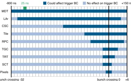
The integration times of the different subdetectors vary significantly, mostly due to the charge drift times depending on the material and geometry of the respective detector system. In most cases, the integration time exceeds 25 ns, i.e. the time between two BCs. In such cases, the signal from events that occurred in previous BCs contaminates the signal in the triggered BC. This is often referred to as out-of-time pile-up and needs to be considered for the simulation, in addition to the in-time pile-up which accounts for signals generated by interactions occurring inside the BC corresponding to the hard-scatter event.
Figure2shows the readout windows considered for the simulation of each of the detector systems. The MDTs have the longest integration time, 750 ns, with 32 BCs prior to the trigger and 6 BCs after the trigger being considered. For the LAr calorimeter it is only slightly shorter. For the inner detector (Pixel, SCT and TRT) the integration time is much shorter, and only the 1–2 BCs before and after the trigger need to be considered.
2ATLAS uses a right-handed coordinate system with its origin at the nominal interaction point (IP) in the centre of the detector and the𝑧-axis along the beam pipe. The𝑥-axis points from the IP to the centre of the LHC ring, and the𝑦-axis points upwards.
Cylindrical coordinates(𝑟 , 𝜙)are used in the transverse plane,𝜙being the azimuthal angle around the𝑧-axis. The pseudorapidity is defined in terms of the polar angle𝜃as𝜂=−ln tan(𝜃/2). Angular distance is measured in units ofΔ𝑅≡
√︃
(Δ𝜂)2+ (Δ𝜙)2.
Figure 2: The time windows considered for the simulation of each subdetector. The dark blue BCs are those where a signal in that BC can contaminate the signal in the triggered BC (i.e. BC 0), while the light blue coloured BCs cannot affect the triggered BC.
3 Overview of simulation chain
As is described above, the ATLAS simulation chain [6], used to produce MC samples to be used in physics and performance studies, is divided into three steps: generation of the event and immediate decays, particle tracking and physics interactions in the detector, based on Geant4 (G4), and digitisation of the energy deposited in the sensitive regions of the detector into voltages and currents to emulate the readout of the ATLAS detector. This simulation chain is integrated into the ATLAS software framework, Athena [18].
Finally, a series of reconstruction algorithms is applied in the same way as for the data, where final physics objects such as jets, muons and electrons are reconstructed [14]. Each step can be run as an individual task, but in order to save disk space the digitisation step is usually performed in the same task as the reconstruction step, such that the intermediate output format from the digitisation step only needs to be stored locally on the computing node and can be discarded after the reconstruction step is finished.
The G4 simulation step is run by itself and, since it is independent of the detector readout configuration, the trigger and the pile-up, it is often run significantly earlier than the digitisation and reconstruction, which depend on these aspects. The G4 simulation is the most CPU intensive and thus it is desirable to run this as rarely as possible.
The ATLAS digitisation software converts the energy deposits (HITS) produced by the G4 simulation in the sensitive elements into detector response objects, known asdigits. A digit is produced when the voltage or current of a particular readout channel rises above a preconfigured threshold within a particular time window. Some of the subdetectors read out just the triggered BC, while others read out several bunch crossings, creating digits for each. For each digit, some subdetectors (e.g. SCT) record only the fact that a given threshold has been exceeded, while others (e.g. Pixel or LAr) also retain information related to the amplitude. The digits of each subdetector are written out as Raw Data Objects (RDOs), which contain information about the readout channel identifier and the raw data that is sent from the detector front-end electronics.
For any given hard-scatter interaction, the additional pile-up interactions must be included in a realistic model of the detector response. For this purpose, minimum-bias events are generated using the Pythia
RDO
(1x) 3) MC Analysis
Reconstruction 2) Digitisation
HITS 1) Simulation (1x)
hard-scatter event
HITS
(~1000x)HITS
(~1000x)HITS
(~1000x)HITS
(~1000x)HITS
(~1000x)
1) Simulation minimum
bias events
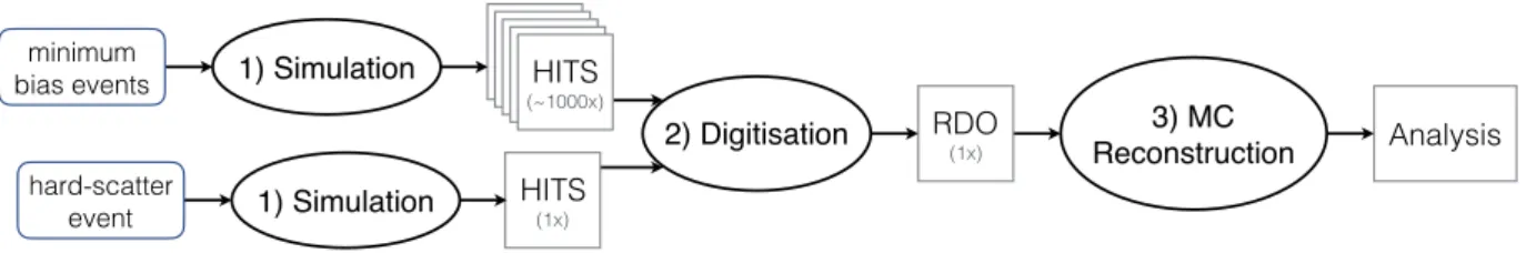
Figure 3: Current workflow diagram from simulation to physics analysis. The oval steps represent an action while the boxes represent data files of a given format. The final box is the reconstructed data in analysis format.
event generator with the NNPDF2.3LO [19] parton distribution function and the A3 [20] set of tuned parameters, then simulated and stored in separate files. In the current standard pile-up simulation chain, the simulation files of both the hard-scatter event and the desired number of minimum-bias events are read in concurrently at the digitisation step and the HITS are combined. For each hard-scatter event a value of 𝜇is assigned by randomly sampling the𝜇distribution corresponding to the relevant data-taking period.
Most subdetector responses are affected by interactions from neighbouring bunch crossings: as is shown in Figure2, up to 32 BCs before and 6 BCs after the triggering BC may contribute signal to the trigger BC. For the average𝜇value of 37.8 during 2017 data taking, this implies that simulating the impact of pile-up on any given hard-scatter event requires approximately(32+1+6) ×38=1482 minimum-bias events on average to be selected at random (from the simulated event files) and processed as part of the digitisation step. Each of these bunch crossings is taken to have the same value of𝜇as the trigger bunch crossing3. The number of minimum-bias events (𝑁) to include for each bunch crossing is drawn at random from a Poisson distribution with a mean of the𝜇value for that bunch crossing. After the energy deposits in the trigger BC due to all contributing BCs have been combined, the detector response is emulated. This workflow is illustrated in Figure3.
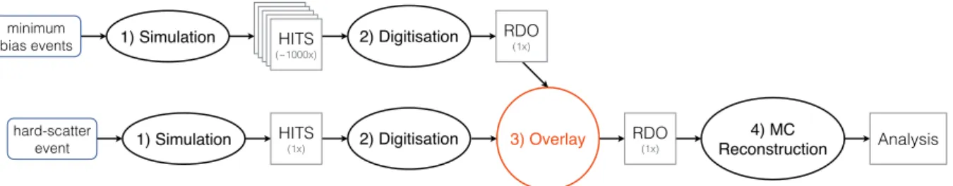
The new presampled pile-up simulation chain is illustrated in Figure4. Rather than digitising the minimum- bias interactions each time a hard-scatter event is produced, a large sample of pile-up events is produced by pre-combining the simulated pile-up interactions, according to the𝜇distribution of the data campaign, during a separate digitisation step, termed presampling4. Here, the sampling is done exactly as for the standard pile-up, the only difference being that there is no hard-scatter event. These presampled pile-up events are written out in RDO format aspile-up RDO datasetsand typically contain several million events.
Each simulated hard-scatter interaction is then digitised and combined with an event sampled from these pile-up datasets (step 3 in Figure4, calledoverlay). Here, instead of HITS for each channel, the signals of the RDO or digit (depending on the subdetector) in the hard-scatter event and the presampled event are overlaid. Since the digitisation, presampling and reconstruction steps are typically combined into a single task in the production workflow, the output is written locally to an RDO file that is then input to the reconstruction software; this local RDO file is subsequently discarded. The pile-up RDO datasets necessary for a given digitisation task are about five times smaller than the many minimum-bias HITS required in the standard pile-up simulation chain.
The main benefit of the presampled pile-up simulation chain is that the CPU and I/O requirements of the digitisation are significantly lower and have a much smaller dependence on𝜇, as is discussed in Section4.
However, if a threshold or compression has been applied to the signal when writing the RDO/digit, this
3In data there are variations between adjacent bunches of order 10% [21] but this is not emulated in the MC simulation.
4For the calorimeters and the SCT, the digitised output stored in the presampled events is amended, so that the presampled pile-up can be applied accurately.
results in some loss of information and thereby could reduce the accuracy of the simulation when using the presampled pile-up method, as is discussed in Sections5–8.
For all the comparisons shown in these sections the hard-scatter events are identical for the two methods but the pile-up events are different. This makes the estimation of the uncertainties difficult as the hard-scatter is fully correlated while the pile-up is not. As most of the quantities are selected to be sensitive to pile-up, the uncertainties are calculated assuming the two samples are uncorrelated but in some distributions this leads to an overestimate of the uncertainties, e.g. in the reconstruction efficiencies of tracks and leptons and in the trigger efficiencies.
Figure 4: The presampled pile-up workflow schema. The oval steps represent an action while the boxes represent data files of a given format. The final box is the reconstructed data in analysis format.
4 Computing performance comparison
In this section the performances of the two simulation chains are compared in terms of CPU time, memory usage and I/O. The validation in terms of physics performance is presented in subsequent sections.
The main computing performance benefit of the presampled pile-up simulation chain stems from the fact a pile-up dataset is only created once per MC production campaign, and then the individual events within that dataset are used for multiple hard-scatter MC samples, as opposed to being created on demand independently for each MC sample. An MC production campaign happens typically once per data-taking period and comprises billions (B) of hard-scatter events and thousands of individual samples. A sample is defined as a set of MC events generated using the same input parameters, e.g. a sample of𝑡𝑡¯events produced by a certain MC generator with a given set of input parameters. The same presampled pile-up event can thus be overlaid on many different hard-scatter events from different MC samples. In doing so, care needs to be taken to ensure that no undesirable effects on physics analyses occur due to reusing the same pile-up events, as is discussed below.
In ATLAS, typically 70% of the CPU resources are devoted to MC production via the simulation chain; the remainder is used for data processing and user analyses. At present, with the Run 2 pile-up profile, the simulation chain CPU usage is broken down into about 15% for event generation, 55% for G4 simulation, 20% for digitisation and 20% for other tasks (reconstruction, trigger, event writing). The presampled pile-up scheme decreases the digitisation time to a negligible level and thus reduces the overall CPU resources required for MC production by about 20%, as is discussed below.
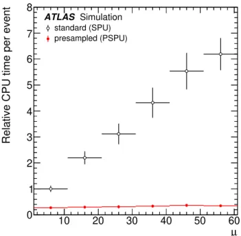
The average CPU time per event in the standard and presampled pile-up simulation chains as a function of 𝜇is shown in Figure5. As can be seen, both depend linearly on𝜇but the slope is about 50 times larger for the standard pile-up than for the presampled pile-up simulation chain. For the standard pile-up simulation chain, the CPU time required at𝜇=70 is 7.5 times larger than for𝜇=10, while for the presampled pile-up
method, the corresponding increase in CPU time is only a factor of 1.2. Extrapolating this to𝜇 =200, the CPU time is 20 times greater than for𝜇=10 for the standard method and< 2 times higher for the presampled pile-up method. However, this comparison does not account for the CPU time required for the production of the presampled pileup dataset, which is needed to assess the overall CPU benefit in a realistic campaign, as is discussed below.
10 20 30 40 50 60
µ 0
1 2 3 4 5 6 7 8
Relative CPU time per event
standard (SPU) presampled (PSPU) ATLAS Simulation
Figure 5: Comparison of the average CPU time per event in the standard pile-up (SPU) digitisation (black open circles) and the presampled pile-up (PSPU) digitisation (red filled circles) as a function of the number of𝑝 𝑝collisions per bunch crossing (𝜇). The CPU time is normalised to the time taken for the standard pile-up for the lowest𝜇 bin. For this measurement𝑡𝑡¯events are used for the hard-scatter event. The average is taken over 1000 events and the vertical error bars represent the standard deviation of the separate CPU time measurements. For the standard pile-up digitisation the slope of the relative CPU time per event versus𝜇is 0.108 while for the presampled pile-up digitisation it is 0.002.
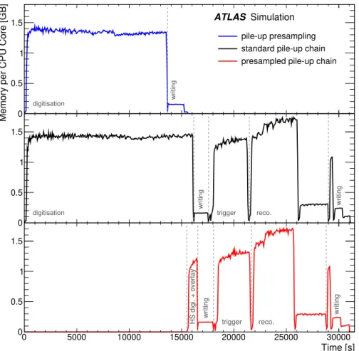
Figure6shows the memory used by the various steps as a function of time for the different production steps for the two simulation chains. The time estimate is based on running 2000 hard-scatter events for the 2017𝜇distribution on the same CPU in all cases, so that the three scenarios can be directly compared. The absolute number, of course, depends on the CPU used and the𝜇distribution. The presampling takes about 70 s per event. The standard digitisation takes about 75 s per event, while the hard-scatter digitisation and overlay of the presampled pile-up takes about 0.5 s. The remaining steps, which are the same for the two simulation chains, take about 8s and include the trigger emulation, reconstruction, and the writing of the analysis format to disk.
When comparing the required CPU time between the two chains, the following equations provide a good approximation. For the standard pile-up simulation chain, the time𝑇standardrequired is simply given by the number of events in the campaign times the total time𝑡digi+𝑡other, where𝑡otheris the sum of the times needed for reconstruction, trigger and writing the event to disk. Thus
𝑇standard =𝑁MC-campaign× (𝑡digi+𝑡other),
where𝑁MC-campaignis the number of hard-scatter events produced in a given MC campaign.
0 0.5 1 1.5
Memory per CPU Core [GB]
digitisation writing
ATLAS Simulation
pile-up presampling standard pile-up chain presampled pile-up chain
0 0.5 1 1.5
digitisation writing
trigger reco.
writing
0 5000 10000 15000 20000 25000 30000
Time [s]
0 0.5 1 1.5
HS digi. + overlay writing
trigger reco.
writing
Figure 6: The memory usage profile of different production steps as a function of the job wall-time for 2000 hard-scatter events. The presampling (top), the standard pile-up (middle) and the presampled pile-up (bottom) simulation chain are compared. In the latter case, “HS digi.” refers to the digitisation of the hard-scatter event. The underlying𝜇distribution is that corresponding to the 2017 data𝜇distribution.
For the presampled pile-up simulation chain, the time𝑇presamplerequired is given by the number of events in the campaign times the time needed for the overlay step and other aspects plus the time required for the presampling. This last contribution is given by the total number of presampled pile-up events required (𝑁pp) multiplied by the event digitisation time, so that the required time is
𝑇presample =𝑁MC-campaign× (𝑡overlay+𝑡other) +𝑁pp×𝑡digi.
The time reduction factor of the presampled pile-up simulation chain compared to the standard is then given by
𝑇presample 𝑇standard
=
𝑁MC-campaign× (𝑡overlay+𝑡other) +𝑁pp×𝑡digi 𝑁MC-campaign× (𝑡other+𝑡digi)
≈ 1
𝑡other+𝑡digi
𝑡other+𝑡digi×
𝑁pp 𝑁MC-campaign
,
where the approximation𝑡overlay 𝑡otheris made, based on the observations from Figure6.
It is immediately clear that the presampled pile-up simulation chain uses less CPU time than the standard pile-up simulation chain since 𝑁pp < 𝑁MC-campaign. Choosing the exact value for 𝑁pp, however, is not trivial. In general, the reuse of a given presampled pile-up event within a particular MC sample, representing an individual hard-scatter physics process, should be avoided if possible, otherwise each overlaid hard-scatter plus pile-up event would not be statistically independent. Suchoversamplingwould be particularly worrisome if the presampled pile-up event in question contained a distinctive feature, such as a high-transverse-momentum jet, which could cause difficulties in using the MC sample for the statistical interpretation of the data distributions. In practice, such a repetition would not be statistically significant in the bulk of a distribution but could be problematic in the tails, where there are few events. Given this, it is reasonable that the value for𝑁ppbe chosen to be about the size of the largest individual MC sample, so that no event is repeated within it.
For the ATLAS Run 2 MC campaign,𝑁MC-campaign∼10 B and the single largest individual MC sample had a size of 0.2 B events. Allowing for some increase in these sizes to be commensurate with the size of the evolving data samples,𝑁pp∼0.5 B should thus be sufficient. Taking the resulting𝑁MC-campaign/𝑁pp∼20, along with𝑡other ≈ 𝑡digi (as seen in Figure 6), the ratio of the times required for the two methods is 𝑇presample/𝑇standard∼0.53. Hence, the presampled pile-up simulation chain provides a CPU saving of 47%
compared to the standard pile-up simulation chain. If the time required for reconstruction and trigger is further improved (as is planned for Run 3), or the digitisation time were to further increase due to pile-up, the ratio would decrease; e.g. if𝑡other≈𝑡digi/2, a CPU saving of 63% would be realised. These are illustrative examples that confirm the intuitive expectation that performing the digitisation just once per campaign is much more effective than doing it for each simulated hard-scatter event, as the number of presampled events needed is by construction smaller than the number of hard-scatter events.
From the memory usage point of view, the presampled pile-up load is similar to the standard pile-up and well below the (soft) production limit of∼ 2 GB per core (see Figure6) for the 𝜇values observed during Run 2 and expected for Run 3. However, compared to the standard pile-up, the presampled pile-up simulation chain puts less stress on the I/O system both because, as is mentioned above, the presampled pile-up dataset files are about a factor of five smaller and because they can be read sequentially. The sequential reading is possible because the random access necessary to combine the minimum-bias input files in the standard pile-up is now performed only once at the presampling stage. Hence, the presampled pile-up RDO production, with its heavier requirements, can be performed on a limited subset of ATLAS MC production sites designed to cope well with such workloads; the subsequent presampled pile-up simulation chain will then run on all resources available to ATLAS, utilising sites that have previously been excluded for reconstruction due to insufficient I/O or disk resources. The smaller I/O requirements from the presampled pile-up simulation chain jobs simplify the production workflow, and make it possible to transfer the pile-up datasets on demand to the computing node at a given production site, where they are needed. If network speed is further increased in the future, it might even be possible to access them directly via the network during the job from a remote storage site.
The Analysis Object Data (AOD) event size written to disk is the same for both methods, i.e. there is neither advantage nor disadvantage in using the presampled pile-up simulation chain in this regard. However, the many simulated minimum-bias events do not have to be distributed as widely any more throughout the year as they only need to be accessed once for creating the presampled events. These presampled events need to be made available widely though. It is expected that these two effects roughly cancel out but operational experience is needed to understand how to distribute the presampled sample in the most effective way.
5 Inner detector
The ID consists of three subdetectors which all use different technologies as discussed in Section2. Each of them has separate digitisation software and hence a different treatment for the presampled pile-up procedure is required for each. In this section, the readout of the three ID subdetectors is described, along with the presampled pile-up procedure for each. Validation results are also presented.
5.1 Detector readout
Silicon Pixel detector: The charge produced by a particle traversing a silicon pixel is integrated if it passes a set threshold. In Run 2, this threshold is typically around 2500 electrons for the IBL and 3500 electrons for the remainder of the Pixel detector. The resulting charge deposited by a minimum-ionising particle (MIP) that traverses a single pixel is typically 16 000 and 20 000 electrons, respectively. The amount of charge deposited by a particle traversing the detector varies depending on the path length of the particle through the active silicon and can be spread across multiple pixels. The length of time during which the charge signal exceeds the threshold, termedtime-over-threshold(ToT), is recorded. The ToT is roughly proportional to the charge. While most of the charge drifts to the pixel readout within the 25 ns bunch crossing time of the LHC, there is a small fraction which may take longer and only arrive in the subsequent bunch crossing (BC+1). Thus, in any given bunch crossing, the pile-up events both from the previous and the current bunch crossings contribute hits.
Silicon microstrip detector (SCT): For the SCT, the readout is in principle similar to the Pixel detector in that a threshold is applied for each strip. But, in contrast to the pixel readout, it is purely digital, i.e.
neither the charge nor the ToT is stored for a given strip, just a bit, X = 0 or 1, to signal a hit (1) or the absence of a hit (0). Hence, the hit from the current BC as well as that of the two adjacent bunch crossings (i.e. BC–1 and BC+1) are read out. Several data compression modes have been used since the first LHC collisions; they are defined by the hit pattern of the three time bins:
• Any-hit mode (1XX, X1X or XX1); channels with a signal above threshold in either the current, previous or next bunch crossing are read out.
• Level mode (X1X); only channels with a signal above threshold in the current bunch crossing are read out.
• Edge mode (01X); only channels with a signal above threshold in the current bunch crossing and explicitly no hit in the preceding bunch crossing are read out.
The data can be compressed further by storing, for adjacent strips with hits above threshold, only the address of the first strip and the number of these adjacent strips. When this compression is invoked, the information about which of the three bunch crossings observed a hit for a given strip is lost. When the LHC is running with 25 ns bunch spacing, SCT RDOs are required to satisfy the 01X hit pattern to be considered during event reconstruction in order to suppress pile-up from the previous crossings.
Transition radiation tracker (TRT): When a particle crosses one of the tubes in the TRT, the electrons drift to the anode wire, producing an electrical signal. If the charge of that signal exceeds a low discriminator threshold, a corresponding hit is recorded, in eight time slices of 3.125 ns each. The drift time is calculated based on the time of the first hit, which is subsequently converted to distance to give a drift-circle radius.
In addition, in order to provide information for electron identification, a record is kept of whether a high discriminator threshold is exceeded in any of the eight time slices. This information is stored for the previous, current and subsequent bunch crossings (i.e. BC–1, BC, BC+1).
5.2 Overlay procedure
The quantities which are overlaid for the inner detector are the RDOs. Due to the high number of channels in the inner detector, zero suppression5 is employed to reduce the amount of data read out and stored from the detector. Since for the ID the RDOs do not contain the full information of the HITS created by simulation, the overlay of RDO information is less accurate than the overlay of the underlying HITS information. However, the impact on physics observables is generally found to be negligible as is described in the following; where a difference is observed, a parameterised correction is derived as is described below.
Pixel detector: The Pixel detector has in excess of 90 M readout channels and a very high granularity.
The single-pixel occupancy is below 2.5×10⁻⁵per unit𝜇in all layers [22], so even at𝜇∼100 it is below 0.25%. Therefore, the chance that a single pixel which contains a signal due to a charged particle from the hard-scatter event also contains one from the overlapping in-time pile-up events is< 0.25%. A pixel RDO contains the channel identifier and a 32-bit packed word containing the ToT, a bunch-crossing identifier, and information related to the L1 trigger not relevant in simulation. In the presampled pile-up, if an RDO of a given channel contains a hit above threshold from either the hard-scatter event or the pile-up event, but not both, the corresponding RDO is kept and written out. In the.0.25% of cases where it contains a hit above threshold in both the hard-scatter event and the pile-up event, only the hard-scatter RDO is kept in order to retain the ToT (and thus, for example, the energy deposited per path length d𝐸/d𝑥) from the signal process. This causes a small loss of information as in principle the ToT would be modified by the presence of the additional charge deposited in that pixel from the pile-up events. But, as it only affects a small fraction of cases, it has a negligible impact on the overall physics performance. In addition, there could be a loss of information if, for a given pixel, both the hard-scatter event and the pile-up event produce charge deposits which are below the readout threshold but whose sum is above the threshold. In this case the presampled pile-up method will register no hit while the standard method will register a hit above threshold. This effect could reduce the cluster size and the ToT. But again, only a very small fraction of pixels are affected, so both the cluster size and the ToT agree well between the two methods.
SCT detector: The SCT is a strip detector with 6.3 M readout channels and an occupancy in high pile-up conditions ofO (1%); consequently the pile-up modelling is more critical than for the pixel detector. In order to facilitate accurate modelling, it is important that presampled RDOs be stored in any-hit mode, without further compression, to ensure that the impact of out-of-time pile-up is modelled correctly. To combine hard-scatter and pile-up RDOs, all of the strips that are hit on a module are unpacked from the respective RDOs and repacked into RDOs using the desired compression mode. Loss of information only
5Rather than reading out all channels, only those channels containing data (above a certain significance level) are recorded.
occurs if hits in both the hard-scatter event and the pile-up event are below threshold but the sum of the two charges is above threshold. In this case, in the standard digitisation a hit would be present while with the presampled pile-up procedure it is not, causing the presampled pile-up procedure potentially to result in fewer SCT hits per track. The impact is, however, negligible as is shown below.
TRT detector: The TRT is a straw tube detector with 320 k readout channels, and in high pile-up conditions the occupancy of the TRT exceeds 10%. Therefore, pile-up has a major impact on the TRT signals. If the channel identifiers in the hard-scatter and pile-up events are the same, the data word stored is set to a bit-wise logical OR of the corresponding raw words. This results in some loss of information as the sum of the charge signals will be larger, and thus more easily pass a given threshold, than would be just the sum of the digitised signals. This particularly impacts the fraction of hits that pass the high discriminator threshold.
A correction for this effect is applied to improve the level of agreement between the presampled pile-up and the standard digitisation. For this correction, a high-threshold (HT) bit is activated according to a randomised procedure, tuned to describe the standard digitisation. The rate of randomly activating a high-threshold bit is parameterised as a linear function of the occupancy of the TRT in the simulated pile-up events (a proxy for the average energy deposited in the pile-up events) and whether the charged particle that is traversing the straw from the hard-scatter event is an electron or not. A different correction is applied for electrons as they produce significant amounts of transition radiation in the momentum range relevant for physics analysis (5–140 GeV), while all other particles do not. The correction corresponds to approximately a 10% (5%) increase in the number of HT hits for electrons (non-electrons) at the average Run 2𝜇value.
5.3 Validation results
To validate the presampled pile-up digitisation for each of the subdetectors, the properties of tracks in simulated𝑡𝑡¯events, where at least one𝑊 boson from the top quarks decays leptonically, are compared between the presampled pile-up method and the standard digitisation. The𝑡𝑡¯events are chosen because they represent a busy detector environment and contain tracks from a wide range of physics objects.
The primary track reconstruction is performed using an iterative track-finding procedure seeded from combinations of silicon detector measurements. The track candidates must have a transverse momentum 𝑝T >500 MeV and|𝜂| <2.5 and meet the following criteria: a minimum of seven pixel and SCT clusters, a maximum of either one pixel or two SCT clusters shared among more than one track and no more than two holes6in the SCT and Pixel detectors combined. The tracks formed from the silicon detector measurements are then extended into the TRT detector. Full details, including a description of the TRT track extensions, can be found in Refs. [23,24].
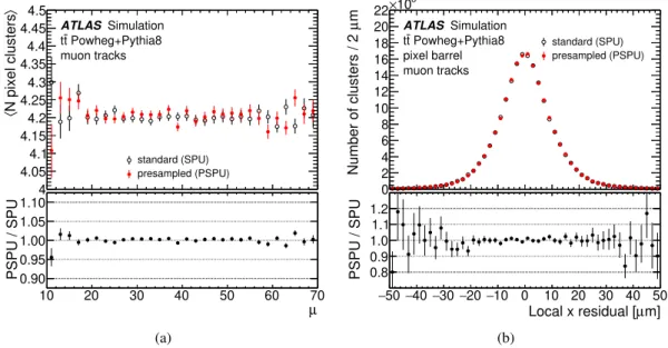
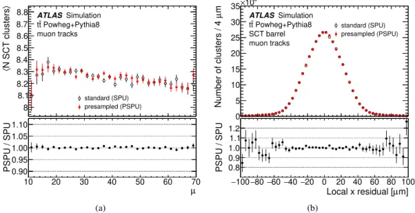
Figure7 shows the number of pixel clusters associated with a muon track as a function of𝜇, and the unbiased residual in the local𝑥coordinate, which corresponds to the direction with the highest measurement precision. The unbiased residual is the distance of the cluster from the track trajectory (not including the cluster itself) at the point where that trajectory crosses the pixel sensor. Figure8shows the corresponding quantities for the SCT. In all cases, the presampled pile-up and standard digitisation are shown, and good agreement is observed between the two methods.
6A hole is defined as the absence of a hit on a traversed sensitive detector element.
4 4.05 4.1 4.15
4.2 4.25 4.3 4.35 4.4 4.45
〉N pixel clusters〈 4.5
standard (SPU) presampled (PSPU) ATLAS Simulation
Powheg+Pythia8 t
t
muon tracks
10 20 30 40 50 60 70
µ 0.90
0.95 1.00 1.05 1.10
PSPU / SPU
(a)
0 2 4 6 8 10 12 14 16 18 20 22
103
mµNumber of clusters / 2 ×
standard (SPU) presampled (PSPU) ATLAS Simulation
Powheg+Pythia8 t
t pixel barrel muon tracks
−50−40−30−20 −10 0 10 20 30 40 50 µm]
Local x residual [ 0.8
0.9 1.0 1.1 1.2
PSPU / SPU
(b)
Figure 7: Comparison of between the standard digitisation (open black circles) and the presampled pile-up (red filled circles), showing (a) the average number of pixel clusters on a track as a function of𝜇and (b) the the local𝑥residuals, for tracks produced by muons in simulated𝑡𝑡¯events. The distributions are integrated over all clusters associated with muon tracks in the hard-scatter event. The residual is defined as the measured hit position minus the expected hit position from the track extrapolation (not including the cluster in question). The bottom panels show the ratios of the two distributions.
Figure9shows a comparison of the number of high-threshold TRT drift circles as a function of 𝜇for muons7 and electrons. As is explained above, due to the high occupancy of the detector, the number of high-threshold drift circles is particularly sensitive to the presampled pile-up procedure. After the parameterised corrections discussed in Section5.2are applied, the average numbers of high-threshold drift circles for electrons and muons are each comparable for the two methods.
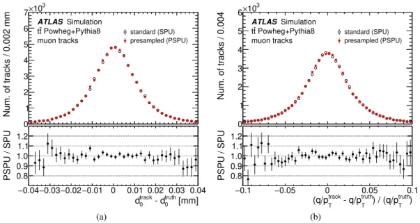
The resolution of all track parameters was examined for both methods, and they were found to agree well.
Figure10shows the difference between the reconstructed and true values for the impact parameter of the track relative to the primary vertex (𝑑0), measured in the transverse plane, and the track curvature (𝑞/𝑝track
T ) for muons in𝑡𝑡¯events. Finally, the track reconstruction efficiency is shown in Figure11as a function of the 𝑝Tand𝜂of all tracks identified in𝑡𝑡¯events. The level of agreement between the two methods is better than 0.5%.
7The proportion of transition radiation, and hence high-threshold hits for pions, which dominate in pile-up events, will behave similarly to muons due to their comparable mass. Muons are chosen here because their momentum spectrum in𝑡𝑡¯events is comparable to that of the electrons and hence allow a direct comparison.
8 8.1 8.2 8.3 8.4 8.5 8.6 8.7
〉N SCT clusters〈 8.8
standard (SPU) presampled (PSPU) ATLAS Simulation
Powheg+Pythia8 t
t
muon tracks
10 20 30 40 50 60 70
µ 0.90
0.95 1.00 1.05 1.10
PSPU / SPU
(a)
0 5 10 15 20 25 30 35
103
mµNumber of clusters / 4 ×
standard (SPU) presampled (PSPU) ATLAS Simulation
Powheg+Pythia8 t
t SCT barrel muon tracks
−100−80−60−40 −20 0 20 40 60 80 100 µm]
Local x residual [ 0.8
0.9 1.0 1.1 1.2
PSPU / SPU
(b)
Figure 8: Comparison of between the standard digitisation (open black circles) and the presampled pile-up (red filled circles), showing (a) the average number of SCT clusters on a track as a function of𝜇and (b) the the local𝑥residuals, for tracks produced by muons in simulated𝑡𝑡¯events. The distributions are integrated over all clusters associated with muon tracks in the hard-scatter event. The residual is defined as the measured hit position minus the expected hit position from the track extrapolation (not including the cluster in question). The bottom panels show the ratios of the two distributions.
1.5 2 2.5 3 3.5 4 4.5
〉N TRT HT drift circles〈 5 standard (SPU)
presampled (PSPU) ATLAS Simulation
Powheg+Pythia8 t
t
muon tracks
10 20 30 40 50 60 70
µ 0.90
0.95 1.00 1.05 1.10
PSPU / SPU
(a)
3.5 4 4.5 5 5.5 6 6.5 7
〉N TRT HT drift circles〈 standard (SPU)
presampled (PSPU) ATLAS Simulation
Powheg+Pythia8 t
t
electron tracks
10 20 30 40 50 60 70
µ 0.90
0.95 1.00 1.05 1.10
PSPU / SPU
(b)
Figure 9: Distributions of the average number of TRT high-threshold drift circles, after the corrections described in the text, for tracks produced by (a) muons and (b) electrons in simulated𝑡𝑡¯events as a function of𝜇. The standard digitisation (open black circles) is compared with the presampled pile-up (red filled circles). The bottom panels show the ratios of the two distributions.
0 1 2 3 4 5 6 7
103
×
Num. of tracks / 0.002 mm
standard (SPU) presampled (PSPU) ATLAS Simulation
Powheg+Pythia8 t
t
muon tracks
−0.04−0.03−0.02−0.01 0 0.01 0.02 0.03 0.04 [mm]
truth
- d0 track
d0
0.8 0.9 1.0 1.1 1.2
PSPU / SPU
(a)
0 1 2 3 4 5 6
103
×
Num. of tracks / 0.004
standard (SPU) presampled (PSPU) ATLAS Simulation
Powheg+Pythia8 t
t
muon tracks
−0.1 −0.05 0 0.05 0.1
truth) ) / (q/pT truth
- q/pT track
(q/pT
0.8 0.9 1.0 1.1 1.2
PSPU / SPU
(b)
Figure 10: A comparison of the reconstructed muon track parameter resolution for (a)𝑑0and (b)𝑞/𝑝Tbetween the standard digitisation (open black circles) and the presampled pile-up (red filled circles) methods, for simulated𝑡¯𝑡 events. The bottom panels show the ratios of the two distributions.
0.86 0.88 0.9 0.92 0.94 0.96
Track reco. efficiency
standard (SPU) presampled (PSPU) ATLAS Simulation
Powheg+Pythia8 t
t
0 5 10 15 20 25 30 35 40 45 50 Track pT
0.995 1.000 1.005
PSPU / SPU
(a)
0.78 0.8 0.82 0.84 0.86 0.88 0.9 0.92 0.94
Track reco. efficiency
standard (SPU) presampled (PSPU) ATLAS Simulation
Powheg+Pythia8 t
t
−2.5 −2−1.5 −1−0.5 0 0.5 1 1.5 2 2.5 Track η 0.995
1.000 1.005
PSPU / SPU
(b)
Figure 11: A comparison of the track reconstruction efficiency between the standard digitisation (open black circles) and the presampled pile-up (red filled circles) methods, for simulated𝑡𝑡¯events as a function of (a) transverse momentum and (b) pseudorapidity (𝜂). All primary charged particles with𝑝T>500 MeV and|𝜂|<2.5 are selected.
The bottom panels show the ratios of the two distributions.
6 Calorimeters
6.1 Detector readout
The standard and presampled pile-up digitisation algorithms are based on an accurate emulation of the readout of the calorimeter system.
For the LAr calorimeter [25], the deposit of energy in the liquid-argon gaps induces an electric current proportional to the deposited energy. For a uniform energy deposit in the gap, the signal has a triangular shape as a function of time with a length corresponding to the maximum drift time of the ionisation electrons, typically 450 ns in the EM calorimeter. This signal is amplified and shaped by a bipolar𝐶 𝑅–(𝑅𝐶)2filter in the front-end readout boards [26] to reduce the effect of out-of-time pile-up energy deposits from collisions in the next or previous bunch crossings. To accommodate the required dynamic range, three different gains (high, medium and low) are used. The shaped and amplified signals are sampled at the LHC bunch-crossing frequency of 40 MHz and, for each L1 trigger, are digitised by a 12-bit analog-to-digital converter (ADC).
The medium gain for the time sample corresponding to the maximum expected amplitude is digitised first to choose the most suitable gain for a given signal. Four time samples for the selected gain are then digitised and sent to the back-end electronics via optical fibres. For the EMB, EMEC and FCAL calorimeters, the position of the maximum of the signal is in the third time sample for an energy deposit produced in the same bunch crossing as the triggered event. For the HEC, it is in the second time sample.
For the Tile calorimeter [27], each cell is read out by two photomultiplier channels. The maximum height of the analogue pulse in a channel is proportional to the amount of energy deposited by the incident particle in the corresponding cell. The shaped signals are sampled and digitised by 10-bit ADCs at a frequency of 40 MHz. The sampled data are temporarily stored in a pipeline memory until an L1 trigger signal is received. Seven time samples, centred around the pulse peak, are obtained. A gain selector is used to determine which gain information is sent to the back-end electronics for event processing. By default the high-gain signal is used, unless any of the seven time samples saturates the ADC, at which point the low-gain signal is transmitted.
6.2 Overlay procedure
The procedure for the LAr calorimeter is described in detail below; a very similar procedure is used for the Tile calorimeter.
In the presampled RDO sample, the pulse shape (ADC data vs time sample) is stored over the time period for which the calorimeter is read out for each calorimeter cell without any zero suppression. Its computation is based on the standard pile-up simulation, described in more detail in Ref. [28]. It considers the energy deposited in each cell for each bunch crossing over the time window affecting the triggered BC, taking into account the time of each event relative to the trigger time. The resulting pulse shape, expressed in energy versus time, is then converted to ADC counts, applying the energy-to-ADC calibration factor per cell and adding the ADC pedestal. The gain used in the readout electronics for this conversion is selected by emulating the logic applied in the front-end readout electronics. The electronics noise is then added to the presampled RDO, with the proper correlation of the noise between the different samples, with a value that depends on the gain used to digitise the pulse.
In the presampled pile-up step, the pulse shape of the presampled event is converted back into energy and then the energy from the hard-scatter event is added. This is done for each time sample, resulting in a combined pulse shape of the hard-scatter and presampled pile-up events. From this summed pulse shape, the energies in each time sample are then converted back to ADC counts to produce a pulse shape mimicking the output of the front-end electronics. The readout electronics gain used in this conversion is selected according to the energies of the summed pulse shape. If this gain differs from the ones used in the hard-scatter or presampled samples, the electronics noise is corrected accordingly.
This pulse shape is then processed following exactly the same algorithm as used in the standard pile-up digitisation, applying the optimal filtering coefficients [29] to estimate the energy per cell [28]. For cells with high enough energy, the time and pulse quality factors are also computed.
Since all cells are stored in the presampled RDO sample without any suppression, and the energy response is perfectly linear in the digitisation, the presampled pile-up does not rely on any approximations except for the integer rounding that is applied when storing ADC counts in the presampled sample. In practice, the impact of ADC integer rounding was found to be almost negligible. This rounding effect only applies to the LAr case; Tile ADC data are actually stored as floats in the presampled RDO sample.
6.3 Validation results
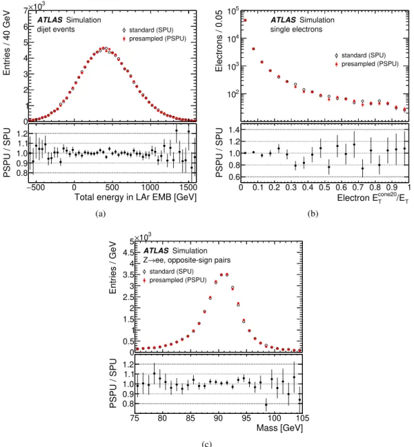
Figure12(a)shows a comparison of the total energy deposited in the EMB calorimeter by dijet events for the presampled pile-up and standard digitisation methods. This distribution is sensitive to electronics and pile-up noise and shows that the simulation of the noise in the two methods is similar. Figure12(b)shows the distribution of a calorimeter isolation quantity𝐸cone20
T /𝐸Tfor simulated single-electron events. This variable is calculated from topological clusters [30] of energy deposits by summing the transverse energies of such clusters within a cone of sizeΔ𝑅=0.2 around (but not including) the candidate electron cluster. It is sensitive to pile-up energy deposits close to the signal electrons and is again similar for the two methods.
Figure12(c)shows the invariant mass distribution of electron–positron pairs from simulated𝑍 →𝑒+𝑒− events. This comparison shows that the energy scale and resolution of electrons from signal events agree for the two methods.
Figure13shows the jet response in𝑡𝑡¯MC events. The jet𝑝Tis calibrated using a multi-stage procedure [31]
that accounts for several effects, including pile-up. The pile-up correction is performed at an early stage of the calibration procedure and removes excess energy due to both in-time and out-of-time pile-up. It is therefore sensitive to the details of the pile-up emulation. The shape of the distribution (which is sensitive to noise modelling) and the average response versus𝜂over the full calorimeter acceptance are in good agreement for the two methods. Also shown in Figure13is the distribution of missing transverse momentum𝐸miss
T for events in the same𝑡𝑡¯sample. Thesoft term component, as reconstructed in the calorimeter, which is particularly sensitive to pile-up [32] is shown as well. Again, good agreement is observed for the two methods.
7 Muon spectrometer
The MS consists of four subdetectors: two providing high-precision tracking measurements and two primarily providing trigger information. The technologies used in these are different and, as with the ID, they require specific digitisation treatments for the presampled pile-up. The main difference in the case
0 1 2 3 4 5 6 7
103
×
Entries / 40 GeV
standard (SPU) presampled (PSPU) ATLAS Simulation
dijet events
−500 0 500 1000 1500
Total energy in LAr EMB [GeV]
0.8 0.9 1.0 1.1 1.2
PSPU / SPU
(a)
102
103
104
105
Electrons / 0.05
standard (SPU) presampled (PSPU) ATLAS Simulation
single electrons
0 0.1 0.2 0.3 0.4 0.5 0.6 0.7 0.8 0.9 1 /ET cone20
Electron ET
0.6 0.8 1.0 1.2 1.4
PSPU / SPU
(b)
0 0.5 1 1.5 2 2.5 3 3.5 4 4.5 5
103
×
Entries / GeV
standard (SPU) presampled (PSPU) ATLAS Simulation
ee, opposite-sign pairs Z→
75 80 85 90 95 100 105
Mass [GeV]
0.8 0.9 1.0 1.1 1.2
PSPU / SPU
(c)
Figure 12: A comparison between the standard digitisation (open black circles) and the presampled pile-up (red filled circles) for (a) the total deposited energy distribution in the electromagnetic barrel of the liquid-argon calorimeter in simulated dijet events, (b) the electron isolation𝐸cone20
T /𝐸Tdistribution for single electrons, and (c) the opposite-sign electron-pair invariant mass distribution from simulated𝑍 → 𝑒+𝑒− events. The normalisation of the figures is arbitrary as it is simply proportional to the number of events in the MC sample. The bottom panels show the ratios of the two distributions.
of the MS compared to the ID is that the occupancy is much lower. This means that, while there is the potential for loss of information in the presampled pile-up method if two sub-threshold hits occur in the same detector channel, the probability of this occurring is much lower and the resulting effect is found to be negligible.