Research Collection
Master Thesis
Functional Encryption for Higher Degree Polynomials assuming Multilinear Maps
Author(s):
Musciagna, Giorgio Publication Date:
2021
Permanent Link:
https://doi.org/10.3929/ethz-b-000477331
Rights / License:
In Copyright - Non-Commercial Use Permitted
This page was generated automatically upon download from the ETH Zurich Research Collection. For more information please consult the Terms of use.
ETH Library
Functional Encryption for Higher Degree Polynomials assuming
Multilinear Maps
Giorgio Musciagna
Supervisors
Prof. Dr. Dennis Hofheinz Bogdan-Gabriel Ursu
Department of Computer Science
1st April 2021
Functional Encryption for Higher Degree Polynomials assuming Multilinear Maps
Giorgio Musciagna ∗ ETH Zürich, Switzerland
Abstract. We present a degree-3 polynomial functional encryption construction which works in the public-key setting and has linear-size ciphertexts. It achieves semi-adaptive simulation security against unbounded collusions and relies on the bilateral K-LIN assumption in prime order trilinear groups. Our construction is also modular, in the sense that relies on lower degree polynomial functional encryption schemes. In particular, we employ functional encryption for computing the linear inner-product and quadratic functions. The usage as underlying building blocks allows to inherit their (simulation) security guarantees. The idea of our construction follows the one initiated by Lin (CRYPTO 17) and later explored further by Gay (PKC 2020) and Wee (TCC 2020), which consists of using inner-product functional encryption to compute extra terms coming from the evaluation of the polynomial functionality on encrypted inputs.
Keywords: Functional encryption, multilinear maps, high degree polynomials, simu- lation security
Contents
1 Introduction 3
1.1 Our contribution . . . . 6
1.2 Technical overview . . . . 6
1.3 Roadmap . . . . 9
2 Preliminaries 9 2.1 Notation . . . . 9
2.2 Groups . . . . 10
2.3 Multilinear maps . . . . 11
2.4 Hardness assumptions . . . . 12
2.5 Kronecker product . . . . 15
2.6 Functional encryption . . . . 16
2.7 Security definitions . . . . 16
3 Degree-3 polynomial functional encryption (3PFE) 18 3.1 Construction . . . . 19
3.2 Simulator . . . . 24
3.3 Security proof . . . . 25
∗
This work is a M.Sc. thesis conducted at ETH Zürich under the supervision of Prof. Dr. Dennis
Hofheinz and doctorate Ursu Bogdan-Gabriel at the Department of Computer Science.
4 Extended inner-product functional encryption (e-IPFE) 54 4.1 Construction . . . . 54 4.2 Simulator . . . . 55 4.3 Security proof . . . . 56 5 Extended degree-2 polynomial functional encryption (e-2PFE) 56 5.1 Construction . . . . 57 5.2 Simulator . . . . 58 5.3 Security proof . . . . 59
6 Acknowledgements 67
A Compact IPFE-only-based 3PFE 70
B Analysis of the [Gay20] quadratic FE 77
1 Introduction
We start by motivating functional encryption [Wat08, BSW10, O’N10]. We do this by taking a step back to the advent of public-key cryptography.
Public-key cryptography was introduced for the first time in 1976 by Whitfield Dif- fie and Martin Hellman [DH76]. A 45 years old invention which at that time revolutionised cryptography. Before then, it was common belief that for two parties to confidentially communicate over an insecure channel, it was necessary to establish a prior mutual secret key between the two. Agreeing on a cipher key in advance was the main issue all cryptosys- tems had at that time. The two parties need to share the cipher key over a secure channel, without having unauthorised parties access the channel. And frequently, the transmission happened through trusted postal services or private couriers, acting as secure channel. In addition to being expensive and slow, this solution is unscalable for communications over larger networks such as the Internet we know today, Internet which in 1976 was very close to its birth. This key distribution issue was solved by Diffie and Hellman who devised a key exchange scheme which did not require any prior shared secret. That was the earliest example of a public-key cryptographic protocol. From there, many public-key based cryptosystems started to appear. Notably, the earliest and well-known are the ElGamal [EG85] and the RSA [RSA78] encryption systems. The impact public-key cryptography hardly can be quantified: its ubiquity in so many applications nowadays is a clear sign.
These range from securing network communications to performing online secure payments, encrypting disks and creating digital signatures.
New technologies, computing advances and potential drawbacks or limitations of ex-
isting cryptographic tools are some of the main drivers in cryptographic research. New
changes clearly lead to a variety of new applications, however existing technologies could
not be sufficient to their realisation. Relatively to security, the question is if existing
cryptographic tools and protocols can still help in providing the necessary security in
protecting data relatively to these new applications. The emerging shift of data to the
cloud and cloud computing is an example nowadays. Suppose an health care center which
has a large online dataset of medical disease records for a large number of patients. This
dataset is naturally encrypted, given the sensitive information it contains. Mining the
dataset giving the ability to some external party to compute aggregate statistics for medical
research without revealing patients’ information for example, is an application one can be
interested in. The question we ask is if a public-key cryptosystem is sufficient to allow such
kind of computation with the above security constraint. Recall, in a public-key setting
every party has a private and a public key. The first is kept private, the second is known to everybody. Public-key encryption can be thought as a padlock with two key slots: one key exclusively locks the pad, the other one only unlocks it. Now, the health care center needs to encrypt the dataset before putting it online. Encrypting it using the private key is useless since everybody could then decrypt the whole dataset using the public one.
Hence, the health care center uses its public-key. Now, imagine we have a set of parties who would like to compute statistics on the encrypted data. What is left to be used is the secret key. And if we do so, we immediately see two issues:
• first, access to the encrypted dataset is all or nothing. That is, if we do not provide the secret key to some party P , then P learns nothing about the dataset. Otherwise, if we give out the secret key to P , then P learns all the content of the dataset.
Clearly, this is not our goal.
• and second, we only have a single secret key which can decrypt the data. Even if we imagine that the secret key would allow the selective computation that P desires without leaking nothing more, what about other parties whose computations might be different from P ’s one?
Public-key encryption does not appear expressive enough for our new application. We are not able to both provide security on the encrypted data and allow decrypting some partial information, or generally speaking a function, of the protected data being encrypted.
Reaching this objective is basically the essence of functional encryption.
Functional encryption. Functional encryption [Wat08, BSW10, O’N10] can be con- sidered as an extension of public-key encryption which enables selective computations on encrypted data. It is a novel paradigm characterised the possibility of generating secret keys sk f for some functions f the requesting party desires, such that decrypting a ciphertext ct x of some private information x with sk f yields f (x). These secret keys are derived from a master secret key, part of a master secret and public key pair. The security of functional encryption lies on the guarantee that if a party holds a set of secret keys sk f
iassociated to several functions f i , he learns nothing about x beyond f i (x). This requirement is also known as collusion resistance. There are two established security definitions which capture this property. The most natural one consists of showing that anything an adversary can compute from ct x and any sk f , she can compute from sk f and f (x). The first scenario is what happens in any real functional encryption scheme. The second is the ideal one, where the ciphertext of x does not appear at all, hence it is completely unknown to the adversary.
This is the essence of the so-called simulation-based SIM security, where one shows that any adversary being in the ideal scenario is not better off in the real scenario. A more traditional indistinguishability-based IND security notion can be also applied. However, the SIM notion is the preferred one: [BSW10] showed that for some functions, insecure functional encryption schemes achieve IND based security. Nonetheless, SIM security is not always achievable. Recall that the IND notion states that an adversary is unable to distinguish encryptions of two messages chosen by herself. This is the standard notion applied to public-key encryption. Specifically to functional encryption, this notion needs however to be slightly extended to avoid trivial wins.
Since 2010 the cryptographic community has doing research on functional encryption trying to devise schemes, based on well understood computationally hardness assumptions, which are both efficient and enable the evaluation of any polynomial time computable function.
Achieving this objective will enable the realisation of the newly emerged applications we
discussed initially such as mining online encrypted dataset, spam filtering systems which
operate over encrypted emails, and many more. However, efficient functional encryp-
tion constructions for general circuits are still out of reach. Currently, we have efficient
schemes for simpler functionalities. In particular, for inner-product and quadratic functions.
Inner-product functional encryption (IPFE). This is notably the most extensively studied case which belongs to efficient functional encryption obtainable from standard assumptions. Functional encryption for inner-products was introduced roughly 5 years ago by [ABDP15] with a practical group-based scheme achieving IND security against selective adversaries (where the adversary sends her challenge input before seeing the public key and asking for secret keys) under the DDH hardness assumption, and a construction based on LWE too. In IPFE a ciphertext is associated to a vector x whereas the functionality associated to a secret key corresponds to a vector y. The decryption algorithm then recovers the weighted sum x > y. Specifically to the group-based IPFE construction under DDH, the inner-product value needs to belong to some polynomially bounded domain which allows efficient computation of the discrete logarithm in the operational group, using for instance the baby step giant step DL-algorithm. The security achieved in [ABDP15]
was later improved by [ALS15] with a slightly modified construction which achieves full IND security (i.e. against adaptive adversaries who can ask for secret keys before seeing the challenge ciphertext) under the DDH, LWE and DCR standard assumptions. This stronger result eventually allowed to shed some light on the SIM security variant since [O’N10] showed that full IND implies non-adaptive simulation security (adversary can ask for secret keys only before seeing the challenge ciphertext). One step forward in this direction was taken by [Wee17] who showed that the full IND [ALS15] construction achieves semi-adaptive simulation (adversary can ask for secret keys only after seeing the challenge ciphertext). However, this result applies only to the DDH-based scheme.
Degree-2 polynomial functional encryption. Additionally to linear functionalit- ies as the inner-product, research has been put on devising efficient constructions based on standard assumptions for evaluating quadratic functions. Keeping the size of the ciphertexts linear in the size of the inputs is a requirement. A construction aimed at computing bilinear maps over the integers was proposed by [BCFG17], with a scheme in the public-key setting based on the standard matrix decisional Diffie-Hellman (D `,k -MDDH, [EHK
+13]) and the 3-party DDH (3-PDDH, [BSW06]) assumptions, achieving selective IND security. Concurrently, [Lin16] proposed a quadratic construction in the secret-key setting based on the standard symmetric external DDH (SXDH) assumption on bilinear maps, which achieves selective IND security too. Recall that a functional encryption scheme in a private-key setting needs the master private key to compute ciphertexts.
Otherwise, the scheme is said to be public-key. An improvement on the security guarantees came roughly last year by [Gay20], who proposed a novel construction in the public-key setting achieving semi-adaptive SIM security proven under the standard SXDH and the bilateral 2-LIN assumptions. A few months later, [Wee20] presented an upgraded version of [Gay20] based on the bilateral 2-LIN assumption, with shorter ciphertexts and without the requirement that the underlying inner-product functional encryption is function-hiding.
Degree-k polynomial functional encryption. As previously mentioned, no efficient
constructions based on standard assumptions are known for general circuits. All proposed
constructions rely on non-standard assumptions such as multilinear maps and indistin-
guishability obfuscation (iO, [BGI
+01]). This means that, efficient schemes for evaluating
functions of degree higher than 2 are still out of reach. Currently, a construction for degree-
k polynomial functions given by [Lin16] exists, but assumes the existence of multilinear
maps. It is also limited to the secret-key setting and achieves selective IND security.
1.1 Our contribution
In this work, we give a degree-3 polynomial functional encryption construction in the public-key setting with linear size ciphertexts, which achieves semi-adaptive SIM security against unbounded collusions and relies on the bilateral 2-LIN assumption in asymmetric prime order trilinear groups. Since we assume the existence of a trilinear map, our work remains of theoretical interest at the moment.
In terms of related works, we recall the previously mentioned work by Lin [Lin16] where a degree-k construction based on multilinear maps is presented too, hence applicable for a degree-3 as in our case. Differently from Lin’s construction which is private-key (due to the underlying function-hiding inner-product functional encryption) and achieves select- ive indistinguishability-based security, our scheme is public-key and enjoys the stronger simulation security in the semi-adaptive setting.
1.2 Technical overview
We proceed by providing an informal overview of our construction. We build a group-based functional encryption scheme for cubic functions, using slightly adapted quadratic and inner-product functional encryption schemes as building block. Recall that any general cubic polynomial can be written as:
q(x, y, z) =
n
X
i=1 m
X
j=1 o
X
k=1
f i,j,k · x i · y j · z k = (x ⊗ y ⊗ z) > f
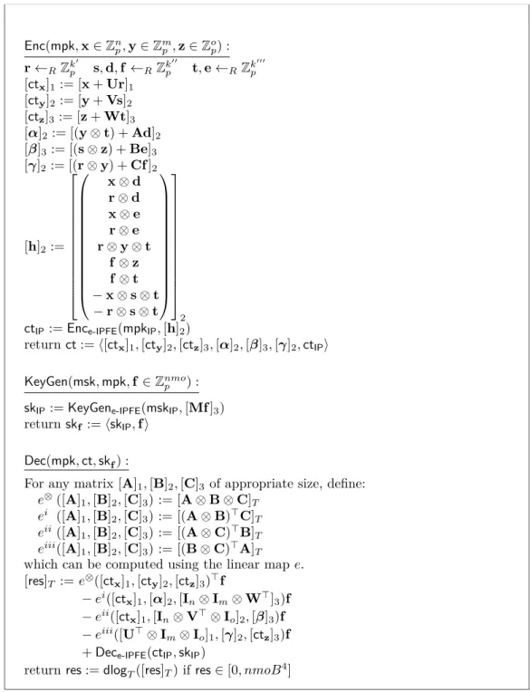
where x ∈ Z n p , y ∈ Z m p and z ∈ Z o p are the input vectors and f ∈ Z nmo p contains coefficients for q(x, y, z). In our cubic functional encryption scheme, ciphertexts are associated with the three input vectors x, y, z since they represent the secret data, whereas secret keys are related to some coefficient vector f a party might ask for. Computing the decryption of the ciphertexts with the secret key reveals only the value (x ⊗ y ⊗ z) > f . For our scheme we rely on the bilateral K-LIN assumption (cf. section 2.4) and on an asymmetric trilinear map e : G 1 × G 2 × G 3 → G T for the trilinear groups G 1 , G 2 and G 3 . We indicate the encoding of x in G a via [x] a using [EHK
+13] notation.
We start by masking the secret vectors x, y and z as follows:
[x + Ur
| {z }
ct
x] 1 , [y + Vs
| {z }
ct
y] 2 , [z + Wt
| {z }
ct
z] 3 ,
where [U] 1 , [V] 2 , [W] 3 are random matrices part of the mpk, and r, s, t are fresh random vectors. We use the pseudo-randomness of vectors [Ur] 1 , [Vs] 2 and [Wt] 3 , implied by the K-LIN assumption, to mask the three inputs. Recall that the K-LIN assumption in a group G a asserts (cf. lemma 2) that, given a random matrix [A] a ∈ G `×K a , then [Aw] a is computationally indistinguishable from a random vector, where w ∈ Z K p is a random vector.
The decryption then computes t 1 := (ct
x⊗ ct
y⊗ ct
z) > f using the trilinear map e which returns:
[ (x ⊗ y ⊗ z) > f + extra terms ] T .
Within the 7 extra terms we can distinguish linear-size and quadratic-size terms. Following the approach in [Lin16, Gay20, Wee20], we express the linear-size extra terms
(x ⊗ Vs ⊗ Wt) > f + (Ur ⊗ y ⊗ Wt) > f + (Ur ⊗ Vs ⊗ Wt) > f + (Ur ⊗ Vs ⊗ z) > f
T
| {z }
t
5using inner-product between two vectors h and Mf as follows:
x ⊗ s ⊗ t r ⊗ ct
y⊗ t r ⊗ s ⊗ z
| {z }
h
>
I n ⊗ V > ⊗ W >
U > ⊗ I m ⊗ W >
U > ⊗ V > ⊗ I o
| {z }
M
f
T
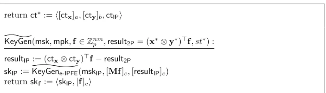
We encrypt [h] 2 and generate a secret-key for [Mf] 3 using a slightly extended version of the standard IPFE, which instead works on trilinear groups and takes group elements as inputs, rather than in plaintext. Similarly in [Wee20], observe that our underlying IPFE does not need to be function-hiding, since the functionality [Mf ] 3 released to the requesting party depends on combined matrices U, V and W in G 3 , matrices which appear always encoded in the mpk. The remaining 3 quadratic-size extra terms
(x ⊗ y ⊗ Wt) > f
T
| {z }
t
2+
(x ⊗ Vs ⊗ z) > f
T
| {z }
t
3+
(Ur ⊗ y ⊗ z) > f
T
| {z }
t
4can be rearranged as:
(x ⊗ (y ⊗ t)) > ((I nm ⊗ W > )f)
T +
(x ⊗ (s ⊗ z)) > ((I n ⊗ V > ⊗ I o )f )
T + +
((r ⊗ y) ⊗ z) > ((U > ⊗ I mo )f )
T
and computed using three copies of a degree-2 polynomial functional encryption, which has been slightly extended to handle trilinear groups. For instance, to compute the term (x ⊗ (y ⊗ t)) > ((I nm ⊗ W > )f
T , we separately encrypt x and y ⊗ t, and we generate a secret-key for
(I nm ⊗ W > )f
3 . Observe, that the we do not require the underlying quadratic functional encryption to be function-hiding, since there is nothing secret about the functionality
(I nm ⊗ W > )f
3 , which can be computed using f and [W] 3 . The final ciphertext is then a tuple consisting of 7 ciphertexts: [ct
x] 1 , [ct
y] 2 , [ct
z] 3 , plus the three ciphertexts relative to the quadratic-size extra terms computed using the extended quadratic functional encryption, and lastly the ciphertext relative to the linear-size extra terms computed using the extended IPFE. The secret-key for a vector f consists of the secret- keys coming from the underlying quadratic and IPFE for the intermediate functionalities (I nm ⊗ W > )f
3 ,
(I n ⊗ V > ⊗ I o )f
3 ,
(U > ⊗ I mo )f
3 and [Mf] 3 . At the decryption time we recover:
(x ⊗ y ⊗ z) > f
T =
(ct
x⊗ ct
y⊗ ct
z) > f
T
| {z }
t
1− (t 2 + t 3 + t 4 + t 5
| {z }
extra terms
)
where t 2 , t 3 t 4 and t 5 come from the decryption of the underlying quadratic and IPFE.
To guarantee simulation security, i.e. make sure that
(x ⊗ y ⊗ z) > f
T is the only informa- tion which leaks from the decryption, the summands t 2 , t 3 t 4 and t 5 have been additionally masked using DDH tuples w i c for i ∈ [1, 4]. This technique has been used in past works too, for instance in [AGRW16, AGW20]. So, we now want instead that:
t 2 := t 2 + w 1 c t 3 := t 3 + w 2 c t 4 := t 4 + w 3 c t 5 := t 5 + w 4 c where:
• the w i ’s are sampled uniformly at random at encryption time, subjected to the constraint P 4
i=1 w i = 0. In this way, at decryption time, the implicit sum of the
masks w i c will result in 0 yielding the original extra terms;
• c is freshly uniformly sampled per secret-key.
So, the linear-size extra terms t 5 are now re-expressed instead as follows:
"
h w 4
>
Mf c
#
T
=
h > Mf + w 4 c
T
For the quadratic-size extra terms, we take as example t 2 which is re-expressed instead as follows:
"
x w 1
⊗ y ⊗ t
1 >
Φ((I nm ⊗ W > )f , c)
#
T
=
(x ⊗ y ⊗ Wt) > f + w 1 c
T
where Φ is a transformation which augments the original functionality (I nm ⊗ W > )f by inserting c at the appropriate positions so that the above equality holds. We provide further details on such a transformation in the correctness of our degree-3 polynomial functional encryption construction in section 3.1.
Security overview. Next, we give a taste on the security for our degree-3 polyno- mial functional encryption. As mentioned earlier, we prove simulation security for our construction (which is stronger than the classical indistinguishability-based security) in the semi-adaptive setting, which means that the adversary can perform post-challenge queries only, i.e. she can ask for secret-keys only after having seen the challenge ciphertexts.
The fact that our scheme uses at its core functional encryption schemes for lower degree- polynomial, namely for linear (inner-product) and quadratic functions, allows us to obtain a modular construction which inherits the security guarantees of its building blocks. In particular, we show that the (extended) inner-product and quadratic functional encryption scheme on which we rely on, both achieve simulation security in the semi-adaptive setting.
The proof of security proceeds via a series of hybrid games:
• First, recall that the ciphertexts ct x , ct
yand ct
zleak no information about x, y and z under the K-LIN, hence can be switched to simulated random ciphertexts.
• We use simulation-security of the underlying building blocks, obtaining input- independent random vectors as simulated ciphertexts and simulated secret-keys where we inject the value of the expected masked extra-terms which should be output at decryption time in case of simulated ciphertexts being provided to the decryption algorithm.
• Then, after having switched the 4 DDH masking terms w i c to random values d i for i ∈ [1, 4], we use a one-time-pad OTP-based change of variable which allows us to collect the 4 non-masked extra terms all together in one of the 4 simulated secret-keys.
Recall, that initially these values were injected separately in each simulated secret-key along with their mask w i c. This enables us to express the non-masked extra terms all together as (ct
x⊗ ct
y⊗ ct
z) > f − (x ⊗ y ⊗ z) > f , i.e. in terms of the simulated random ciphertexts and the output of the cubic functionality (which is the only input-dependent data that the simulation security notion permits).
On the adaptive SIM security and arbitrary degree polynomials. Lastly, we would like to shed some light on two natural questions.
The first one concerns the achievement of SIM security in the adaptive setting. We
previously stated that our scheme achieves semi-adaptive simulation security. This is
inherited from its real core building block, which is actually the inner-product functional
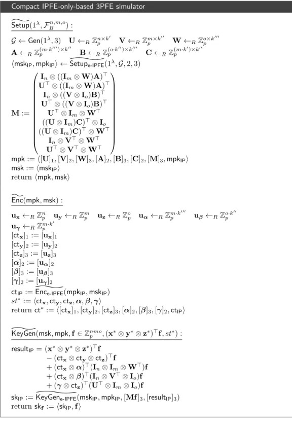
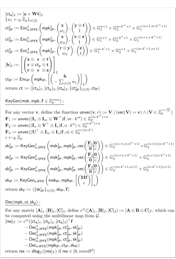
encryption (the quadratic scheme we use as additional underlying block is itself based on IPFE too). Indeed, we can construct a more compact version of our degree-3 polynomial functional encryption we present in this paper, based instead only on IPFE (which we show in appendix A). Recently, [ALMT20] showed that [ALS15] IPFE actually achieves adaptive simulation security without any modification on the scheme. The new simulator they propose is an improvement on [Wee17]’s one, where the generation of the simulated ciphertext is changed. For almost a decade, improving the security of IPFE appeared quite challenging, given that [BSW10, AGVW13] showed that straightforward adaptations appear impossible in the adaptive setting. The fact that we inherit the security of IPFE since it is our core building block and that its security has been improved by [ALMT20] in the adaptive setting without any change to the original scheme, let us conclude that our degree-3 construction (as well as the already existing quadratic schemes based on IPFE) can achieve adaptive SIM security too.
The second question we might ask is about extending to arbitrary degree-k polynomials.
As being modular in the approach, a generalisation to a degree-k polynomial appears possible, although we have not investigated particularly in this direction, given our reliance on multilinear maps (whose constructions are still unknown) which makes our research of theoretical interest at the moment. However, one observation which comes from attempting to extend to degree-k polynomials using the same approach used in our cubic scheme is the following. For a K-LIN-based degree-k polynomial, the ciphertext coming from the underlying IPFE is the largest one, having length O(n · K k−1 ). For simplicity, we assume that the input vectors are all of length n. The value for K cannot be lower than 2 if we consider asymmetric multilinear maps. This means, that a straightforward extension of our approach based on IPFE as building block as initiated by [Lin16, Gay20, Wee20] would lead to a non-linear ciphertext.
1.3 Roadmap
The rest of this paper is structured as follows. After recalling some preliminaries in section 2, we present our degree-3 functional encryption scheme followed by its simulator and security analysis in section 3. Its building blocks, namely the extended inner-product and quadratic functional encryption, are given in section 4 and 5 along with the simulator and the security proof too. Additionally, we give in appendix A a compact self-contained description of our degree-3 polynomial functional encryption based solely on IPFE as a building block. As extra, we also provide in appendix B an observation on the [Gay20]
quadratic functional encryption construction.
2 Preliminaries
This section defines notions and definitions which will be used throughout this paper.
2.1 Notation
Let Z denote the set of integers and N the set of positive integers. We define Z p as the
set of remainders modulo p, namely {0, . . . , p − 1} with p being prime. For finite sets and
bit-strings, | · | denotes their cardinality and length, respectively. For a positive integer
n, we denote by [n] the set {1, . . . , n}. We use boldface lowercase letters to name column
vectors x = (x i ) > and boldface uppercase letters for matrices A = (a ij ). The notation
s ← R S stands for sampling an element s ∈ S according to the uniform distribution over
the finite set S. If D is a probability distribution, then x ← D means x being selected
according to D. The security parameter is denoted by λ ∈ N and the notation 1 λ means
a string of λ ones. A negligible function negl(x) is a function which is smaller than the
inverse of any polynomial in x. More formally, negl : N → R + such that for every positive polynomial poly(x), ∃x 0 ∈ N | ∀x > x 0 : negl(x) < poly(x) −1 . We say that some event happens with overwhelming probability if its probability equals 1 − negl(n). Unless stated otherwise, all algorithms are probabilistic polynomial time, in short PPT. A PPT algorithm A is one which is randomised, i.e. has the ability to flip coins, and its running time is polynomially bounded by the length of its input, i.e. there exists a polynomial poly(·) such that the running time of A on input a bit-string x ∈ {0, 1} ∗ is less than poly(|x|). Given two algorithms A and O, the notation y ← A O(·) (·) means that we assign to y the output of A which runs on some inputs and has access to oracle O. We use the symbol ≈ c to denote computational indistinguishability between two probability distributions. We use the symbol ≈ s to denote statistical indistinguishability between two distributions. We write tuples by listing the elements within angle brackets.
2.2 Groups
A group is a mathematical structure h G ;
F, ei equipped with a non empty set G , a binary operation
F: G × G → G and a special element e ∈ G called identity or neutral element.
A group must satisfy the following three properties.
• Associativity: ∀a, b, c ∈ G : a
F(b
Fc) = (a
Fb)
Fc
• Identity: ∀a ∈ G : a
Fe = e
Fa = a
• Inverse: ∀a ∈ G : ∃ˆ a | a
Fˆ a = ˆ a
Fa = e
A group is abelian or commutative if its binary operation commutes, i.e. ∀a, b ∈ G : a
Fb = b
Fa. Two groups h G ;
F, e 1 i and h H ; , e 2 i are isomorphic, denoted by G ∼ = H , if there exists a bijection φ : G → H , called isomorphism, such that φ(a
Fb) = φ(a) φ(b) for all a, b ∈ G . Isomorphisms are generally difficult to compute efficiently. Given a finite group G , the order of G represents the number of its elements, in short | G |.
Conventions and notations. The above definition of groups tries to capture as much as possible the abstractness behind the concept of a group: note that the elements of a group might not be necessarily numbers. Same reasoning also applies to the associated binary operation, hence the usage of some unconventional and general symbols such as the above
F
, ˆ · and e. Nonetheless, these symbols are rarely used in practice: the already existing notation for addition and multiplication operations has been borrowed instead, obtaining two well-established notation conventions one can freely choose to represent arbitrary groups. These are the additive and the multiplicative notation. The multiplicative notation can be used when working with any group, whereas the additive one only if the group is abelian. The table below summarises the two notations.
additive notation multiplicative notation
F
+ ·
e 0 1
ˆ
a −a a −1
a
Fb a + b a · b or ab
a
Fa
F. . .
Fa
| {z }
k-times
k · a or ka a k
In the subsequent sections of this paper, we will use the additive notation when performing operations on group elements.
Cyclic groups. Consider a finite group G . This is said to be cyclic if there exists
an element g ∈ G such that every element a ∈ G can be obtained as g
Fg
F. . .
Fg k-times
for k ∈ N (in multiplicative notation, we would say that ∀a : a = g k ). If this is true, then
we denote by G = hgi the fact that G is a finite cyclic group having g as a generator. As
corollary, recall that by an important theorem, ∀a ∈ G : a
Fa
F. . .
Fa | G |-times is equal to the identity element e (in additive notation, we would say that ∀a : | G | · a = e). Finally, note that cyclic groups are abelian.
Examples of groups. A standard example of a group is h Z ; +, 0i having as set the set of the integers Z , addition as binary operation, 0 as identity element, and the inverse of an element a denoted by −a following the additive notation which best suits this group structure. Another known group is h R \ {0}; ·, 1i having as set the set of the reals R except 0 since 0 has no inverse, multiplication as operation, 1 as identity element, and the inverse of an element a being denoted by a −1 according to the multiplicative notation.
Representing elements in groups. In cryptography, cyclic groups are generally used to encode numerical values into group elements. Suppose some a ∈ Z p and a cyclic group G = hgi of order p. The encoding (or implicit representation) of a in G is denoted by [a] := g
Fg
F. . .
Fg a-times. In multiplicative notation [a] := g a , in additive notation [a] := ag. The bracket notation [·] was firstly introduced in [EHK
+13]. When working with more than one group G i , the notation simply modifies to [a] i ∈ G i . The bracket notation can be also extended to matrices (and vectors) as follows. For any A = (a ij ) ∈ Z n×m p , we define [A] as the implicit representation of A in G , pointwise:
[A] :=
[a 11 ] . . . [a 1m ] .. . .. . [a n1 ] . . . [a nm ]
∈ G n×m
The motivation behind representing elements in groups is the existence of several complexity problems on groups which allow us to construct and prove security of a cryptographic scheme if we assume the intractability of these problems for any PPT adversary. The root of all group-based hardness assumptions is the DL assumption which states that it is computationally hard to recover a from a uniformly chosen [a] ∈ G , where the integer a is unique and known as the discrete logarithm of [a] in G . Performing operations on data over its encodings is of prominent importance. In particular, we can homomorphically compute addition and multiplication by some scalar over encoded data. Formally, for any given scalar c ∈ Z p and any given encoding [a], [b] ∈ h G = hgi;
Fi, we can efficiently compute:
[a + b] = [a]
F[b]
[c · a] = [a]
F[a]
F. . .
F[a]
| {z }
c-times
without knowing a and b. One can easily prove the two equalities above by expanding the terms using the definition of [·]. Computing multiplication on data over encoded data, i.e.
computing [ab] from just [a] and [b], appears however to be computationally hard. This belief is actually the CDH assumption: given some uniformly chosen [a] and [b], computing [ab] is intractable for any PPT adversary.
2.3 Multilinear maps
We say that e : G 1 × G 2 × · · · × G k → G T is a k-linear map if it satisfies the three properties below. Note that we use multiplicative notation (2.2) for this definition.
• The groups G 1 , G 2 , . . . , G k , G T are of the same prime order
• For any a i ∈ G i and x i ∈ Z where i ∈ [k], then:
e(a x 1
1, a x 2
2, . . . , a x k
k) = e(a 1 , a 2 , . . . , a k ) Q
ki=1
x
i• The k-linear map e is non-degenerate: if ∀i ∈ [k] we have g i being a generator for G i , then e(g 1 , g 2 , . . . , g k ) is a generator for G T
Additionally, e must be efficiently computable and, for security purposes, the DL problem in any group must be hard. The definition of cryptographic multilinear maps given above is a generalisation of the notion given by Boneh and Silverberg [BS02] where they consider only the symmetric case, i.e. the case where G 1 = G 2 = · · · = G k . Rothblum [Rot12] also considered the asymmetric case where the groups may be different. In this paper, we work with asymmetric k-linear groups, i.e. with k different cyclic groups for which we assume the existence of an efficiently computable asymmetric k-linear map and that no efficiently computable isomorphism φ : G i → G j exists for any i, j ∈ [k].
Current state of multilinear maps. At the present time however, known efficiently computable multilinear maps exists only for k = 2, i.e. for bilinear maps (also known as pairings), which can be efficiently obtained using the Weil and Tate pairings on el- liptic curve. Additionally, [BS02] showed that all natural generalisations of pairings from algebraic geometry to build valid k-multilinear maps for k > 2 are not efficiently com- putable by polynomials as in the Weil or Tate pairing. Much effort has been put in the last decade to devise alternative multilinear map construction candidates, for instance [GGH12, CLT15, GGH14] based on graded encoding schemes, especially considering that the holy-grail cryptographic primitive iO (indistinguishability obfuscation [BGI
+01]) can be obtained from multilinear maps. Unfortunately, all candidate graded encoding schemes have been broken [MSZ16, HJ15, CLLT15, CHL
+14, CLR15] so far, leaving the construc- tion of efficient multilinear maps still an open problem. Apart from iO, multilinear maps represent on their own also a valid constructive tool to achieve many other interesting applications [BS02, FHPS13, PTT10] which act as motivation to continue working on this open problem. Relatively to constructing efficient multilinear maps, recall that iO implies multilinear maps too. Thus, we lastly mention some recent advances made towards constructing provable secure iO which does not rely on heuristics and conjectured new hardness assumptions. These new constructions have not been crypto-analysed yet. In particular, with the line of works [LV16, Lin16, JS18, AJS18, JLMS19, AJL
+19], the assumptions needed to construct iO have been reduced to pairings and PRGs with some peculiar properties. Very recently, [JLS20] presented a construction for iO using pairings, based on the Learning With Errors (LWE), Learning Parity with Noise (LPN), SXDH, and assuming the existence of a PRG in NC 0 (recall, NC 0 is the class of functions which are computable by constant-depth, bounded fan-in circuits).
For now, in this paper, we assume the existence of k-linear maps which behave as an extension of the Weil or Tate pairings.
2.4 Hardness assumptions
Next, we recall the complexity assumptions used in this work. Let Gen be an algorithm which takes as input 1 λ , some positive k ∈ N and returns a description G of a k-linear group setting, which is the setting we work with in this paper.
G := hp, { G i } i∈[k] , {g i } i∈[k] , G T , ei ← Gen(1 λ , k)
where ∀i ∈ [k] ∪ {T } : G i is of prime order p > 2 λ . In addition, ∀i ∈ [k] : G i = hg i i. Lastly, e : G 1 × G 2 × · · · × G k → G T is a k-linear map defined in section 2.3. In our work, e is an asymmetric linear map.
DDH assumption. The decisional Diffie-Hellman assumption holds relative to G in
G i for some i ∈ [k] if for all PPT adversaries A the following distinguishing advantage is
negligible in λ, where the probabilities are taken over G ← Gen(1 λ , k) and a, b, c ← R Z p . Adv DDH G,
Gi,A (λ) := |Pr[1 ← A(G, [a] i , [b] i , [ab] i )] − Pr[1 ← A(G, [a] i , [b] i , [c] i )]| = negl(λ) It is easy to see that the DDH assumption implies, i.e. reduces to, the CDH assumption which in turn implies the DL assumption. In short, DDH = ⇒ CDH = ⇒ DL. This is proved by easy reductions. For instance, to see why DDH = ⇒ DL, one usually proves the logically equivalent ¬DL = ⇒ ¬DDH, which means that if we assume that DL is easy, then DDH is easy too. Indeed, suppose one has oracle access to a DL solver. Then, any challenge hG, [a] i , [b] i , [c] i i can be answered correctly with probability 1 by asking the DL oracle for the discrete logarithms a, b of [a] i , [b] i and then checking if [c] i equals [ab] i . This means that the DDH problem surely can not be harder, i.e can be potentially easier, than the DL problem. Hence, the DDH assumption offers stronger security guarantees than the DL assumption. Lastly, recall that the DDH assumption is false in symmetric multilinear groups: if G := G 1 = G 2 = · · · = G k , then e is a symmetric k-linear map e : G k → G T . By linearity of e, any adversary can solve DDH in G by checking if:
e([a], [b], [1], . . . , [1]) = [ab] T = [c] ? T = e([c], [1], . . . , [1])
Considering instead asymmetric multilinear groups, it is easy to see that the DDH assump- tion holds in some group G i as long as we do not provide the encodings of the challenge also in one other group G j6=i or more. To see more clearly why this is the case, consider the minimal case of providing to the adversary a DDH challenge both in groups G i and G j6=i for which there exists an asymmetric (k ≥ 2)-linear map. This challenge variant formally translates to the bilateral DDH assumption in both G i and G j , which states that:
hG, [a] i , [b] i , [ab] i , [a] j , [b] j , [ab] j ]i ≈ c hG, [a] i , [b] i , [c] i , [a] j , [b] j , [c] j ]i
for a, b, c ← R Z p and G ← Gen(1 λ , k). Showing that the bilateral DDH is actually false in asymmetric (k ≥ 2)-linear groups is relatively straightforward. W.l.o.g. we assume that i < j. Similarly to the symmetric case, any adversary can win any bilateral DDH challenge as follows: she can solve DDH in G i by computing and checking if:
e([1] 1 , . . . , [a] i , . . . , [b] j , . . . , [1] k ) = [ab] T = [c] ? T = e([1] 1 , . . . , [c] i , . . . [1] k ) and she can solve DDH in G j by similarly computing and checking if:
e([1] 1 , . . . , [b] i , . . . , [a] j , . . . , [1] k ) = [ab] T
= [c] ? T = e([1] 1 , . . . , [c] j , . . . [1] k )
The notorious and increasing relevance of pairings (and more generally multilinear maps, if shown to exist at some point) in many cryptographic applications, and the fact that one of the most well-understood standard assumptions as DDH turns out actually to be in part false, have led to the proposal of new (now standard) assumptions believed to be true in multilinear groups, which informally generalise DDH. These are presented below.
K-LIN assumption. The K linear assumption for some K ∈ N holds relative to G in G i for some i ∈ [k] if for all PPT adversaries A the following distinguishing advantage is negligible in λ, where the probabilities are taken over G ← Gen(1 λ , k) and a 1 , . . . , a K , x 1 , . . . , x K , c ← R Z p .
Adv K-LIN G,
Gi,A (λ) :=
Pr[1 ← A(G, [a 1 ] i , ..., [a K ] i , [a 1 x 1 ] i , ..., [a K x K ] i ,
K
X
j=1
x j
i
)]
− Pr[1 ← A(G, [a 1 ] i , ..., [a K ] i , [a 1 x 1 ] i , ..., [a K x K ] i , [c] i )]
= negl(λ)
The first definition of this assumptions came originally for K = 2. Boneh, Boyen and Shacham [BBS04] proposed a new decisional assumption for bilinear groups as a con- sequence of the fact that DDH in such setting is easy due to the symmetric pairing. This assumption named decisional linear DLIN assumption actually corresponds to the 2-LIN assumption. Later on, [HK07, Sha07] generalised the DLIN to the K-LIN assumption for K-linear groups. Note also that the 1-LIN = DDH. For different values of K, one actually obtains a family of increasingly weaker assumptions, i.e. harder problems. In other words:
1-LIN = ⇒ 2-LIN = ⇒ · · · = ⇒ K-LIN. The 1-LIN is the easiest problem, hence offers the strongest security guarantees. The K-LIN is the hardest problem, hence offers the weakest security guarantees. Along the lines of what said for DDH, the K-LIN assumption holds in symmetric (k ≤ K)-linear groups and is false in symmetric (k > K)-linear groups.
The K-LIN assumption holds in asymmetric (k ≤ K)-linear groups as in the symmetric case, but it also holds in asymmetric (k > K)-linear groups as long as we do not provide the encodings of the K-LIN challenge in a total of l > K groups for l ∈ [k]. That is, the (l > K)-lateral K-LIN assumption is false in asymmetric (k > K)-linear groups.
D `,k -MDDH assumption. Let `, k ∈ Z p with ` > k. We call D `,k a matrix distribu- tion if it outputs with overwhelming probability and in polynomial time matrices in Z `×k p
of full (column) rank k. The notation D k stands for D k+1,k . The D `,k -MDDH assumption holds relative to G in G i for some i ∈ [k] if for all PPT adversaries A the following distin- guishing advantage is negligible in λ, where the probabilities are taken over G ← Gen(1 λ , k), A ← D `,k , w ← R Z k p , u ← R Z ` p .
Adv D G,
`,k-MDDH
Gi
![Figure 3: Extension of the SA-SIM D k -MDDH-based IPFE construction by [Wee17] which takes into account group element inputs in a (k ≥ 2)-linear group setting G.](https://thumb-eu.123doks.com/thumbv2/1library_info/3908840.1525986/55.892.159.729.568.986/figure-extension-construction-account-element-inputs-linear-setting.webp)
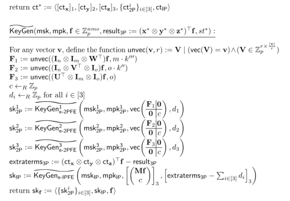
![Figure 4: Simulator for the extended SA-SIM D k -MDDH-based IPFE by [Wee17].](https://thumb-eu.123doks.com/thumbv2/1library_info/3908840.1525986/57.892.155.738.154.221/figure-simulator-extended-sim-mddh-based-ipfe-wee.webp)
![Figure 5: Generalisation of the SA-SIM 2PFE construction by [Wee20] to a (k ≥ 3)-linear group setting G.](https://thumb-eu.123doks.com/thumbv2/1library_info/3908840.1525986/58.892.154.732.256.875/figure-generalisation-sim-pfe-construction-linear-group-setting.webp)