Country Clustering in Comparative Political Economy
John S. Ahlquist and Christian Breunig
Max Planck Institute for the Study of Societies, Cologne May 2009
MPIfG Discussion Paper ISSN 0944-2073 (Print) ISSN 1864-4325 (Internet)
© 2009 by the author(s)
John S. Ahlquist is a Postdoctoral Fellow at the Institute for Research on Labor and Employment, University of California Los Angeles. Christian Breunig is an Assistant Professor at the Department of Political Science, University of Toronto.
jahlquist@irle.ucla.edu c.breunig@utoronto.ca
MPIfG Discussion Papers are refereed scholarly papers of the kind that are publishable in a peer-reviewed disciplinary journal. Their objective is to contribute to the cumulative improvement of theoretical knowl- edge. The papers can be ordered from the institute for a small fee (hard copies) or downloaded free of charge (PDF).
Downloads www.mpifg.de
Go to Publications / Discussion Papers
Max-Planck-Institut für Gesellschaftsforschung Max Planck Institute for the Study of Societies Paulstr. 3 | 50676 Cologne | Germany
Tel. +49 221 2767-0 Fax +49 221 2767-555 www.mpifg.de info@mpifg.de
classifying countries into one of a small number of categories based on their economic institutions and policies. The most recent of these is the Varieties of Capitalism project, which posits two major clusters of nations: coordinated and liberal market economies.
This classification has generated controversy. We leverage recent advances in mixture model-based clustering to see what the data say on the matter. We find that there is considerable uncertainty around the number of clusters and, barring a few cases, which country should be placed in which cluster. Moreover, when viewed over time, both the number of clusters and country membership change considerably. As a result, argu- ments about who has the “right” typology are misplaced. We urge caution in using these country classifications in structuring qualitative inquiry and discourage their us- age as indicator variables in quantitative analysis, especially in the context of time-series cross-section data. We argue that the real value of both Esping-Andersen’s work and the Varieties of Capitalism project consists of their theoretical contributions and heuristic
classification of ideal types.
Zusammenfassung
In der vergleichenden Politischen Ökonomie reicher Demokratien gibt es eine lange Tra- dition, Länder aufgrund ihrer unterschiedlichen wirtschaftlichen Institutionen und Po- licies zu typologisieren. Die jüngste dieser Typologien – das „Varieties-of-Capitalism“- Konzept – erfasst zwei Gruppen von Ländern: koordinierte und liberale Marktwirt- schaften. Da diese Klassifizierung einige Kontroversen hervorgerufen hat, nutzen die Autoren neueste Fortschritte im „mixture model-based clustering“, um zu prüfen, wel- che Erkenntnisse die Daten zu diesem Problem liefern. Die Ergebnisse weisen eine be- trächtliche Unsicherheit hinsichtlich der Anzahl der Cluster und, mit wenigen Ausnah- men, der Zuordnung der Länder zu Clustern auf. Betrachtet man größere Zeiträume, variieren darüber hinaus die Anzahl der Cluster und Ländermitgliedschaften erheblich.
Als Folge dieser Befunde halten die Autoren Argumentationen über die „richtige“ Ty- pologisierung für unangebracht und raten davon ab, diese Länderklassifizierungen zur Strukturierung qualitativer Studien heranzuziehen oder als Indikatorvariablen in quan- titativen Analysen zu nutzen. Dies gilt insbesondere im Kontext von gepoolten Zeitrei- hen- und Querschnittsdaten. Sie argumentieren, dass der substanzielle Wert sowohl der Forschung von Esping-Andersen als auch des „Varieties-of-Capitalism“-Ansatzes in den Beiträgen zur Theorie und den heuristischen Klassifizierungen von Idealtypen besteht.
Contents
Introduction 5
1 Welfare regimes and institutional complementarities:
Clustering in comparative political economy 6
Where do these clusters come from? 8
Empirical application of the VoC classification 9
2 Cluster analysis and the social sciences 10
Hierarchical and relocation clustering methods 10
Mixture model-based clustering 12
3 Three worlds, two varieties, and the data 17
MMBC applied to pre-selected variables and indices 18
Data 21
Clustering with variable selection 24
Clustering within major substantive areas 25
Clustering with sampled country-years 28
Two further methodological considerations 30
4 Discussion and conclusion 31
References 33
Data Appendix 37
Introduction
The remarkable variation in both political-economic institutions and outcomes across industrial democracies has provided fodder for political economists for at least a half century. To make sense of this variation, a long and distinguished tradition emerged of classifying countries into one of a small number of categories. Among the most in- fluential works is Esping-Andersen’s (1990), which sorts rich democracies into “three worlds” labeled Liberal, Conservative, and Social Democratic. The “varieties of capital- ism” project (Hall/Soskice 2001), henceforth VoC, builds on the “three worlds” approach by incorporating insights from the new institutional economics, but shifts emphasis to the role of the firm. The VoC literature argues that these same twenty-odd countries can be assigned the labels of either “liberal market economy” (LME) or “coordinated mar- ket economy” (CME). This dichotomy is so intuitively compelling that it has begun to structure empirical research, both quantitative and qualitative. On the quantitative side, indicator variables representing whether a particular country is an LME have appeared as regressors (Ringe 2006; Rueda/Pontusson 2000; Taylor 2006), sometimes in an ef- fort to explain a variable that others have cited as determining the initial classification (Hamann/Kelly 2009). On the qualitative side, the VoC logic has been used to justify case selection as well as the dimensions for comparative case study (Campbell/Pedersen 2007; Culpepper 2007; Thatcher 2004).
To date, this exercise in classification has been the result of rankings on additive indices and expert judgments along a large number of dimensions. Unsurprisingly, the cluster- ing of countries has generated a fair degree of controversy. Are there only two varieties of capitalism? Where should we put Portugal? Are these categories immutable, at least over the period from 1980 to the present? Indeed, Thelen (2004: 2) states that “all these various categorization schemes also have trouble sorting the same set of ‘intermediate’
or hard to classify countries.” The purpose of this article is to tackle questions about classification of countries theoretically and empirically.
In this paper, we leverage recent advances in mixture model-based clustering (Fraley/
Raftery 1998, 2002; Raftery/Dean 2006) to see what the data say on the matter. By posit- ing the data as a mixture of some to-be-estimated number of multivariate Gaussian densities, the mixture model approach gives cluster analysis a strong basis in probability theory. In so doing, model-based clustering has three notable advantages over tradi- tional clustering methods. First and most importantly, the choice of clustering method now becomes a problem of model choice. We have strong guidance from well-under- stood principles of likelihood theory in this regard. Second, the model-based approach identifies the number of clusters in the data. Other methods either require a priori as- sumptions (e.g., k-means) or only describe how “far” various observations are from one another (agglomerative clustering). Third, model-based clustering can accommodate several cluster shapes; traditional methods are special cases of the more flexible cluster geometries available in the model-based approach.
In the analysis, we identify the dimensions along which countries are purported to vary and collect time-series measures on each for 21 OECD countries, 1980–2005. We then examine these data for clusters both in the cross-section and over time. We find that the data parallel the experts’ arguments: There is considerable uncertainty around the number of clusters and, barring a few cases, over which country should be placed in which cluster. Moreover, when viewed over time, both the number of clusters and coun- try membership change considerably. Therefore, we urge caution in using country clas- sifications in empirical analysis.
We have two objectives in this paper. First, we hope to expand the use of mixture models in the social sciences by applying them to a substantive controversy. Second, our findings have several implications for the literature in comparative political economy. Specifically, arguments about who has the “right” typology are misplaced; these data do not exhibit sufficient structure for any time-invariant all-encompassing clustering to be empirically useful. Therefore discussions of LMEs or CMEs should be used as heuristics or Weberian ideal types only. These categories do not measure anything meaningful in the data ana- lytic sense, especially in the context of time-series cross-section data, and should there- fore not be employed as indicator variables. Finally, we argue that the real value of both Esping-Andersen’s work and the varieties of capitalism project persists in their theoreti- cal contributions, which have been largely obscured by easy-to-remember typologies.
The paper proceeds in four parts. Section 1 briefly reviews the long tradition of classifi- cation in comparative political economy (CPE), with an emphasis on the controversies and uses of the VoC and “three worlds” perspectives. Section 2 discusses mixture models and model-based clustering in more detail, with special attention to their relationships to other clustering and data reduction techniques commonly used in the social sciences.
Section 3 explores the variables purported to define the VoC clusters and discusses the limits of our analysis. We conclude in Section 4 with observations on how best to em- ploy the theoretical insights from the VoC project in empirical research, given our find- ings from the cluster analysis.
1 Welfare regimes and institutional complementarities:
Clustering in comparative political economy
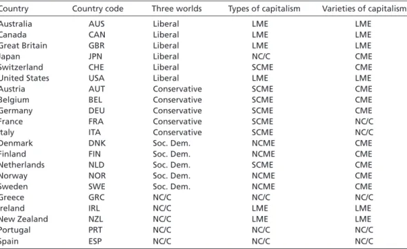
Attempts to generate typologies of advanced democracies started in the late 1950s with the distinction between residual and institutional welfare states (Wilensky/Lebeaux 1958). Literature on corporatism continued this proclivity for developing country typologies and made it a mainstay in political science (see Siaroff 1999 for a recent example).1 The most recent classifications, presented in Table 1, are the motivation for 1 We thank Martin Höpner for pointing out this trajectory.
our paper. The table lists the classification of 21 advanced democracies according to Esping-Andersen’s (1990) three worlds of welfare states, Kitschelt et al.’s (1999) insti- tutional diversity of contemporary capitalism, and Hall and Soskice’s (2001) firm-cen- tered classification of varieties of capitalism.
We do not intend to review the theoretical arguments surrounding the three worlds and VoC classifications, but there is a significant empirical implication worth describing.
Broadly speaking, each of these attempts at clustering is driven by theoretical arguments positing self-reinforcing linkages across economic policies and institutions. Esping-An- dersen refers to these linkages as “regimes” of welfare state effort and traces their emer- gence to the form of cross-class coalitions emerging in the postwar period. Specifically, he focuses on the choice of the new middle class as determining the type of welfare state regime that later emerged. The VoC literature is based on the notion of “institutional complementarities” in which “the presence (or efficiency) of one [institution] increases the returns from (or efficiency of) the other” (Hall/Soskice 2001: 16). These institutional externalities reinforce (or undo) one another and generate distinct equilibrium clusters of institutional arrangements, corporate strategies, and social policies and outcomes.
Both the historical arguments of Esping-Andersen and the strong notions of equilibrium in the VoC literature directly imply that clusters of countries should be time-invariant or, at the very least, should change very slowly. Much of the recent work in the VoC literature aims to discover how resilient these clusters are in the face of exogenous changes in the international economy (Campbell/Pedersen 2007; Culpepper 2005; Thatcher 2004).
Table 1 Twenty-one OECD economies and their categorizations
Country Country code Three worlds Types of capitalism Varieties of capitalism
Australia AUS Liberal LME LME
Canada CAN Liberal LME LME
Great Britain GBR Liberal LME LME
Japan JPN Liberal NC/C CME
Switzerland CHE Liberal SCME CME
United States USA Liberal LME LME
Austria AUT Conservative SCME CME
Belgium BEL Conservative SCME CME
Germany DEU Conservative SCME CME
France FRA Conservative SCME NC/C
Italy ITA Conservative SCME NC/C
Denmark DNK Soc. Dem. NCME CME
Finland FIN Soc. Dem. NCME CME
Netherlands NLD Soc. Dem. SCME CME
Norway NOR Soc. Dem. NCME CME
Sweden SWE Soc. Dem. NCME CME
Greece GRC NC/C NC/C NC/C
Ireland IRL NC/C LME LME
New Zealand NZL NC/C LME LME
Portugal PRT NC/C NC/C NC/C
Spain ESP NC/C NC/C NC/C
Note: The country codes are based on ISO 3166. The country classifications are: LME = Liberal Market Economy, CME = Coordinated Market Economy, NCME = National Coordinated Market Economy, SCME = Sectoral Coordinated Market Economy, NC/C = not categorized or controversial.
Where do these clusters come from?
The inspiration for clustering in the comparative political economy literature springs from the stark differences in labor market organization, social spending, and firm struc- ture across the relatively successful countries of Western Europe, North America and the Pacific basin. While Germany and the United States are frequently contrasted as archetypal cases for VoC, the major theoretical works emphasize that the typologies are meant to generate Weberian ideal types through which to evaluate actual cases, not specific empirical groupings. Hall and Soskice (2001: 8) state that “the core distinction we draw is between two types of political economies … which constitute ideal types at the poles of a spectrum along which many nations can be arrayed.” Nevertheless, these same works also attempt to empirically identify clusters and map them onto their ideal types. Many subsequent authors seem to have taken up the empirical clustering more than the theoretical arguments.
Before turning to some of the empirical applications of the VoC classification, let us briefly consider how the initial clusterings were generated. The typologies have emerged from two major sources: direct comparison of a set of countries along a limited number of dimensions and expert classifications. We focus on the former. Esping-Andersen con- structed several additive indices of decommodification, corporatism, pensions, etc. for circa 1980 and then ranked countries using these indices. He finds that certain groups of countries tend to jointly rank highly on some indices and near the bottom on others.
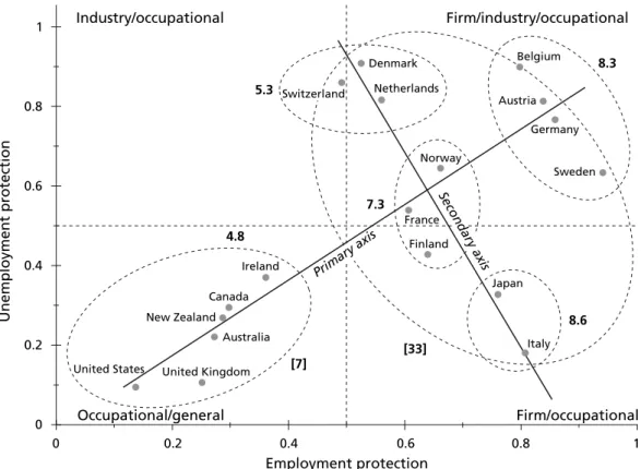
On this basis he argues for his three worlds. The earlier VoC works tend to rely on visual heuristic methods that are also frequently based on additive indices and specific time points. Figure 1, from Estévez-Abe, Iversen and Soskice (2001), is an example of a visual classification of countries according to the level of social protection and skill formation.
We will return to these data and this plot below.
Subsequent authors have attempted to revise these classifications. Some have disputed the placement of certain countries, most notably the southern European economies of France, Spain, and Portugal, and argued for the inclusion of a “Latin” or “Mediter- ranean” regime (e.g. Saint-Arnaud/Bernard 2003: 504). Others have proposed similar revisions (Amable 2003; Obinger/Wagschal 2001). Alternatively, a second dimension of classification has been proposed (Höpner 2007). Most directly related to our proj- ect, several papers attempt to put the VoC classifications on more rigorous footing us- ing data reduction techniques such as principal components analysis (Hicks/Kenwor- thy 2003), latent factor analysis (Hall/Gingerich 2004), traditional clustering methods (Obinger/Wagschal 2001; Saint-Arnaud/Bernard 2003), or all three (Amable 2003).
Schröder (2008) has even proposed integrating VoC and welfare regimes using cluster analysis. We discuss how our analysis extends these exercises in detail below.
Empirical application of the VoC classification
The empirical applications of the VoC arguments have focused on either exploiting the VoC classification scheme, testing it, or, in at least one instance (Taylor 2006), exploiting the VoC classifications to argue against the VoC theoretical apparatus. VoC classifica- tions have been employed empirically in both quantitative and qualitative analysis.
On the quantitative side, dummy variables representing cluster membership have been either directly included as regressors (Ringe 2006; Taylor 2006) or used to split the data- set into parts and then test for the equality of coefficient estimates across models fit to data from CMEs and LMEs (Rueda/Pontusson 2000). All these analyses use time-series cross-section (TSCS) data and treat cluster membership as time-invariant. In this paper we do not attempt to show the extent to which these authors’ findings are sensitive to cluster allocation, but it is worth mentioning that Taylor (2006) shows that findings relating patent counts to VoC clusters are sensitive to the inclusion of the United States as an LME.
Note: This is figure 4.2 from Estévez-Abe/Iversen/Soskice (2001: 172).
Unemployment protection
Industry/occupational Firm/industry/occupational
Occupational/general
Employment protection
Firm/occupational
Denmark Netherlands Switzerland
Norway
Belgium
Austria Germany
Sweden
France Finland
Japan
Italy United States United Kingdom
Australia New Zealand
Canada Ireland
5.3
7.3
8.3
8.6 4.8
[7] [33]
Secondary axis
Primary axis 1
0.8
0.6
0.4
0.2
0
1 0.8
0.6 0.4
0.2 0
Figure 1 Heuristic visual clustering
The VoC classification has, if anything, found its broadest application in qualitative work. Indeed, while the initial clustering of countries was shown heuristically in bivari- ate scatterplots, the most extensive discussion of empirical differences in Hall and Soskice’s introduction was a comparison of the United States and Germany. Case stud- ies have most frequently used the VoC classification to justify case selection. To take a few recent examples already mentioned above, Thatcher (2004) argues that his choice of cases for comparing telecommunications regulations (Germany, France, Italy, Great Britain) is driven by their positions in the VoC pantheon. Campbell and Pedersen (2007) use the VoC classifications to justify both the choice of case (Denmark) and dimensions of analysis (labor markets, vocational training, and industrial policy). The journal Gov- ernance recently dedicated an entire issue to comparisons of economic crisis manage- ment in Japan and Sweden. The introduction (Immergut/Kume 2006) specifically in- vokes the VoC in justifying this emphasis.
2 Cluster analysis and the social sciences
Cluster analysis (and its close relative, discriminant analysis) is a well-developed branch of applied statistics that attempts to identify groups in data such that objects within groups are as similar as possible while the differences between groups are maximized.
Cluster and discriminant analysis have found wide application across disciplines as di- verse as botany, chemistry, computer science, genetics, geography, medicine, and zoolo- gy. Within the social sciences, cluster analysis has appeared most frequently in sociology but has been less common in political science and economics. In this section we briefly introduce traditional cluster analysis and then go into a detailed discussion of the mix- ture model-based clustering (MMBC) approach we employ below. We then contrast MMBC analysis to both traditional methods and other data-reduction techniques, as well as to latent-variable models such as principal components and factor analysis.
Hierarchical and relocation clustering methods
Throughout we will use the term “group” to refer to the true, existing groupings of objects and “cluster” to denote the collections of observations identified via some algo- rithm or statistical model, i.e., a cluster is an estimated grouping. Cluster analysis has at least one of two objectives: identifying some sort of cluster structure in a set of ob- servations and/or assigning observations to clusters in some optimal manner. Kaufman and Rousseeuw (1990) offer an accessible introduction to traditional cluster analysis.
Relocation methods,2 k-means being the most well-known, require that the researcher 2 Sometimes, they are confusingly referred to as partitioning methods.
posit the number of clusters in the data a priori and then proceed to iteratively move observations between clusters until an optimal allocation can be identified. In hierar- chical cluster analysis, the number of groups is unknown. Hierarchical cluster analysis uses intuitively plausible procedures based on various distance metrics to either merge or partition observations into clusters.
Hierarchical cluster analysis can take one of two forms. The “agglomerative” approach starts by regarding each object on its own and proceeds to combine them into clusters that maximize within-cluster similarity and between-cluster difference, as determined by a distance metric. Several different metrics can be employed here, and the literature provides little guidance about their appropriateness. The “divisive” approach proceeds in the opposite direction, beginning with all objects in one cluster and subdividing them until each object is on its own. Frequently these methods yield different solu- tions.3 Presentation of hierarchical clustering results is most commonly done through dendrograms, where the length of line segments is directly interpretable as the dissimi- larity between clusters. The longer the segment before two clusters combine into one, the more dissimilar the observations.
Hierarchical cluster analysis is primarily an exploratory rather than confirmatory or inferential activity. There are many attributes on which to measure similarity and dif- ference across objects, and numerous algorithms for identifying clusters given some set of attributes. There is no statistical basis on which to prefer a particular clustering solu- tion over another and no possibility of evaluating the uncertainty around a particular observation’s assignment to a given cluster. The choice of both the number of clusters to focus on and the substantive interpretations assigned to them is solely the responsibility of the researcher. Referring to the traditional clustering methods, Venables and Ripley (2002: 316) argue that “there are many different clustering methods, often giving differ- ent answers, and so the danger of over-interpretation is high.”
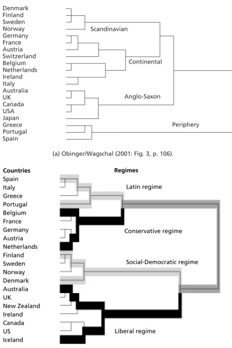
The hierarchical approach has been applied at least twice to problems similar to the one we address below (Obinger/Wagschal 2001; Saint-Arnaud/Bernard 2003). Though these authors analyze somewhat different sets of data and use slightly different time frames, both conclude that there are four relevant clusters among advanced industrial nations, though the exact membership varies across studies and time. Figure 2 displays some results from both papers.
As can be seen from Figure 2, it is up to the researcher to identify, justify, and interpret a four-cluster solution. A two-, five-, or six-cluster solution seems just as plausible for both dendrograms in Figure 2. Traditional methods provide no principled way out of this problem.
3 The divisive approach is much less common, as its computational demands increase exponen- tially in the number of observations (Venables/Ripley 2002).
Mixture model-based clustering
Mixture models have a long tradition in statistics and have more recently been ap- plied to the clustering problem by Fraley and Raftery (1998, 2002) and Raftery and Dean (2006). This second generation of clustering methods assumes that the observed data are generated by some finite mixture of probability distributions.
Countries Spain Italy Greece Portugal Belgium France Germany Austria Netherlands Finland Sweden Norway Denmark Australia UK
New Zealand Ireland Canada US Iceland
Regimes Latin regime
Conservative regime Conservative regime
Liberal regime
Social-Democratic regime Denmark
Finland Sweden Norway Germany France Austria Switzerland Belgium Netherlands Ireland Italy Australia UKCanada USAJapan Greece Portugal Spain
Continental
Anglo-Saxon
Periphery Scandinavian
(a) Obinger/Wagschal (2001: Fig. 3, p. 106).
(b) Saint-Arnaud/Bernard (2003: Fig. 4, p. 513).
Figure 2 Illustrative results from two studies relying on traditional hierarchical clustering
Let x = x1…xn be the n × k matrix of n objects measured along k dimensions. The den- sity of x can then be expressed as a finite mixture model of the form
f g f
g G
( )x = g( )x
å
= p 1where G is the number of groups, πg is the proportion of objects in group g, and fg (∙) is the density function for observations in group g. We assume that all groups are defined by multivariate normal densities, yielding
f g
g G
( )x = ( | )x g
å
= p f q 1where φ (∙|θ) is the multivariate normal density function with parameters θg = (µg,Σg). The model classifies an observation as being in group g if τg (x) > τh (x) ∀h ≠ g; h ∈1,…,G where
t p f q
p f q
g g g
h h G
h
( ) ( | )
( | )
x x
x
=
å
= 1τg can be interpreted as the (posterior) probability that an observation belongs to group g. We can now express the full mixture likelihood:
( , , ; , ,q1 q t1 t | ) t f( | )q
1 1
¼ ¼ =
=
=
å Õ
G G g
g G
i n
i g
x x (1)
It is clear from equation 1 that the number of parameters estimated grows rapidly with the number of clusters G and the number of dimensions k. Baneld and Raftery (1993) partially mitigate this problem by placing restrictions on the covariance matrices Σg. Covariance matrices are parameterized using eigenvalue decompositions of the form
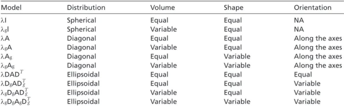
Sg =lgD A Dg g Tg (2) where λg is the largest eigenvalue of Σg, Dg is the orthogonal matrix of eigenvectors, and Ag is a diagonal matrix of scaled eigenvalues. The parameters θg determine the geometry of the clusters. Specifically, clusters are ellipsoids centered at the mean vector. The de- composition of Σg determines other geometric features of the clusters: λg determines the cluster’s volume; Dg controls the orientation of the cluster; and Ag governs the shape of the ellipsoid. MMBC admits a wide variety of cluster geometries.
We can modify the complexity of the models estimated by restricting the various com- ponents of the matrix product on the RHS of equation 2 to be constant across clusters.
The most restricted version, Σg = λI, constrains clusters to be spherical and of equal
volume.4 Table 2, reproduced from Fraley and Raftery (2007: 7), describes the various cluster geometries generated as restrictions on the covariance matrices are relaxed.
In fitting the model, the actual cluster to which observation i belongs is treated as miss- ing data. The “complete data” xi can be expressed as xi = (yi,zi) where yi are the ob- served data on which we seek to fit the clustering model and zi is a G-vector, the gth element of which takes on 1 if i belongs to cluster g and 0 otherwise. Assuming that zi
~multinom(τ1…τG ), the resulting complete data likelihood is given by
c g g i g z
g G
i n
= ig
=
=
Õ
Õ
[t f [( | )]]y q1 1
(3) (3) is maximized via EM (Dempster/Laird/Rubin 1977). For the M-step, (3) is maxi- mized wrt (τ1,…τG; θ1…θG), holding z at z~ . Given estimates (τ ~g , θ ~g ), z~ g is given from the E-step:
t f q
t f q
g g i g
h h G
h i h
( | ) ( | ) y
y
å
= 1(4)
For the multivariate normal mixtures used here, Fraley and Raftery (2002) give closed form solutions for τ~g and μ~g : τ~g = ng/n, where ng = Σ ni=1 z~ig, and μ~g = (Σ ni=1 z~ig yi )/ng.
Model choice and MMBC
The challenge of MMBC is to select both the number of clusters and the parameteriza- tions of the covariance matrix. Since each combination of these choices represents a (non-nested) statistical model, MMBC recasts the clustering problem as one of model selection. We have strong guidance from statistical theory in this regard: Non-nested 4 Note that this is equivalent to the sum-of-squares distance measure most frequently employed
in hierarchical clustering (Ward 1963).
Table 2 Cluster geometries generated by differing parameterizations of the covariance matrices Σg
Model Distribution Volume Shape Orientation
λI Spherical Equal Equal NA
λgl Spherical Variable Equal NA
λA Diagonal Equal Equal Along the axes
λgA Diagonal Variable Equal Along the axes
λAg Diagonal Equal Variable Along the axes
λgAg Diagonal Variable Variable Along the axes
λDADT Ellipsoidal Equal Equal Equal
λDgADTg Ellipsoidal Equal Equal Variable
λgDgADTg Ellipsoidal Variable Equal Variable
λgDgAgDTg Ellipsoidal Variable Variable Variable
models can be compared using approximate Bayes factors (Kass/Raftery 1995).5 Bayes factors are frequently difficult to integrate so we use the Bayesian information criterion (BIC) approximation
BIC = –2log(x, θ ) + m log n
where θ is the maximum likelihood estimate of θ and m is the number of free param- eters in the model. In comparing models, we choose the parameterization(s) that maxi- mize the BIC. Conventionally, two models with a BIC difference less than two are dif- ficult to distinguish, whereas a difference of ten or greater constitutes strong evidence for favoring one model over another (Kass/Raftery 1995).
Variable selection and MMBC
Any collection of objects can be measured and classified according to a large number of attributes (or dimensions). This is especially true when looking at complex entities, such as nations, over time. Intuitively, one can imagine that as the number of dimen- sions approaches the number of objects to be classified there must be increasingly tight clustering to discern any pattern in the data.6 Technically, as the number of dimensions increases so does the number of parameters to estimate for θ, imposing constraints on the effective number of dimensions we can consider.7 In our application, we have a maximum of 21 cases for any point in time. Even restricting attention to “just” the stan- dard variables of comparative political economy (industrial and labor market structure, social policy, and political-economic institutions) we still have to consider literally doz- ens of potential attributes and several different measures for each attribute. It is simply not feasible to simultaneously consider all the plausible or proposed variables when determining the varieties of capitalism.
It is worth noting that this problem is implicit in the major works classifying countries.
Esping-Andersen relies on a small number of constructed indices to identify his “three worlds.” The VoC literature rarely considers more than two particular attributes at a time. Some authors have resorted to data reduction techniques: Hicks and Kenworthy (2003) rely on principal components to reduce the dimensionality of the data in order 5 The Bayes factor is the posterior odds for one model compared to another under the assump- tion that there is no prior reason to favor one over another. Formally, let M1 and M2 be two competing models and y be the data. The Bayes factor is given by
p y p y
p p y d
p p y d
( | ) ( | )
( | ) ( | , ) ( | ) ( | , )
1 2
1 1 1 1 1
2 2 2 2
=
ò ò
q q q
q q q22
6 As a simple example, consider two points on a page. On what basis can we say there is one clus- ter or two?
7 How quickly this constraint prevents EM convergence clearly depends on the restrictions im- posed on Σg. Agglomerative methods suffer from the same problem; it is merely less transparent here, since there is no underlying statistical parameterization to consider.
to classify different modes of welfare capitalism. Hall and Ginderich (2004) perform factor analysis on a cross-section of data and interpret the first factor extracted as repre- senting the CME-LME division. Amable (2003) goes even further, conducting agglom- erative analysis on the first three principal components.
Traditional data reduction techniques and cluster analysis do not easily go together.
Chang (1983) proves that clustering information is not monotonically related to the eigenvalues of the principal components. There is no reason to believe that principal components with the largest eigenvalues are those retaining the greatest amount of clustering information. Reducing the dimensionality of the data by selecting principal components with the largest eigenvalues and then performing a cluster analysis, wheth- er mixture model, hierarchical or relocation clustering, is usually not justified.
The MMBC-model selection approach provides one way around this problem. Raftery and Dean (2006) extend the notion of BIC-based model selection to include variable selection. They develop an algorithm in which the data, Y, are partitioned into three sets: variables already selected for clustering (Y1), variables being considered for inclu- sion or exclusion from Y1, denoted Y2, and all remaining variables (Y3). The algorithm is initialized by choosing the variable on which there is the most evidence of cluster- ing. With each subsequent step, two models are considered.8 In the first step, Y2 gives no additional information on clustering conditional on Y1. In the second, Y2 does im- prove clustering. At each step the models are compared and a variable is included or excluded based on its effect on the BIC, maximized over the number of clusters and model parameterizations.9 Moreover, the variable selection procedure provides a way in which to use dimension reduction techniques, such as principal components. The MMBC algorithm, applied to principal components, chooses the extracted component with the greatest amount of clustering information rather than the one that maximizes
“explained” variance, as the eigenvalue criterion does.
To summarize the discussion on clustering and MMBC: To date, social scientists at- tempting to classify rich democracies have employed methods best characterized as exploratory. We see unstable results and findings that hinge on the researchers’ inter- pretations. These works implicitly avoid dimensionality problems by relying on addi- tive indicators or data reduction techniques such as principal components analysis. In contrast, the MMBC and model selection approach improves previous efforts by (1) allowing for more flexible clustering geometries based on well-understood parametric distributions; (2) providing a principled way for selecting the optimal clustering solu- tions by comparing non-nested models via the BIC; (3) generalizing the variable selec- 8 Formally, we are interested in models characterizing p(Y|z), where z defines cluster member-
ship. Model 1 factors this into p(Y3|Y2,Y1)p(Y2|Y1)p(Y1|z) whereas model 2 posits p(Y3|Y2,Y1) p(Y2,Y1|z).
9 The maximum number of clusters must be set prior to analysis. For our application below we set this maximum to seven unless otherwise noted. See Raftery/Dean (2006: 176–177) for a detailed elaboration of the algorithm.
tion problem to one of model selection, thereby providing guidance on which variables to use, be they single variables or principal components.
3 Three worlds, two varieties, and the data
In this section we use the MMBC approach to explore the data for clustering structure and compare our findings with assertions from both Esping-Andersen’s “three worlds”
approach and the varieties of capitalism approach. Before turning to the data analysis, we outline our rationale for data selection. First, in order to keep the gap between theoretical concepts and operationalization as small as possible, we replicate data used in key stud- ies. Second, we assemble a large batch of variables that previous works have identified as relevant for distinguishing countries. Specifically, we follow the theoretical development in the VoC literature. We start with the core dimensions of the VoC approach – the pro- duction regime measures as identified in Hall and Gingerich (2004). From there, we fol- low the literature on advanced capitalist democracies, including three areas. First, we in- clude measures of welfare, because of the proposed link between production regime and welfare states (Iversen 2005; Mares 2001; Swenson 2002). A second strain of literature adds the importance of political institutions (Gourevitch/Shinn 2005; Iversen/Soskice 2006; Iversen/Stephens 2008). Finally, recent efforts (Soskice 2007) link the production regime with macroeconomic policy.
We approach the analysis in steps.10 We begin by using MMBC to explore the clustering reported in Figure 1 (Estévez-Abe/Iversen/Soskice 2001: 172) and Hall and Gingerich (2004). Both these analyses are static and we use them to illustrate the value-added of the MMBC approach even when our findings are similar in flavor to the VoC clustering.
We next describe the data we have gathered and then take a more dynamic perspec- tive, employing MMBC and the variable selection algorithm to look at cross-sectional slices at different time periods. We then show that our non-finding of stable clustering solutions over time corresponding with either the VoC or “three worlds” approaches is robust for clustering on different subsets of variables. Rather than using the variable selection directly, we break the variables into institutional/policy domains and consider clustering within each of those. Finally, to put the temporal stability argument to an even stronger test, we randomly select a time slice for each country and examine these temporally mixed datasets using MMBC. Across all these analyses, we find little evi- dence of clustering of the form described by literature on either “three worlds” or VoC.
A few words on the presentation and interpretation of results are in order. Our goal here is not to attempt to identify specific clusters and impose any interpretation on them;
rather, we are concerned with determining the empirical robustness of typology devel- 10 All analysis was performed in R 2.6.1 (R Core Development Team, 2007) using the mclust,
mclust02, and clustvarsel libraries (Fraley/Raftery 2002, 2007; Raftery/Dean 2006).
oped elsewhere. Wherever possible, we attempt to present results graphically in which clusters are identified by the density contours of the estimated cluster distribution. This has the advantage of visually displaying the uncertainty surrounding each point, but be- comes impossible when clustering in more than two or three dimensions. In these cases we report tables of results. When evaluating clustering solutions, we frequently come upon situations in which the MMBC/model selection procedure identifies solutions with either only one cluster or more than six as the best-fitting model. We interpret either of these solutions as demonstrating the absence of any interpretable clustering structure in the data.
MMBC applied to pre-selected variables and indices Clustering of welfare production regimes
Before turning to the dynamic analysis, we illustrate the MMBC approach on two static datasets. In this section, we apply MMBC to variables already identified as defining welfare production regimes. The data are those reported in Estévez-Abe, Iversen and Soskice (2001), Iversen (2005: ch. 2), and summarized in Figure 1. As a first step, we apply the variable selection algorithm to their original six variables: three variables on employment protection and three on unemployment protection, using collective dis-
Table 3 Clusters of welfare production regimes
Country Cluster Uncertainty
CAN 1 0.00
FIN 1 0.00
FRA 1 0.00
NOR 1 0.00
SWE 1 0.00
AUT 2 0.00
BEL 2 0.00
CHE 2 0.00
DEU 2 0.00
DNK 2 0.00
NLD 2 0.00
IRL 3 0.01
JPN 3 0.00
NZL 3 0.00
AUS 4 0.00
GBR 4 0.00
ITA 4 0.00
USA 4 0.00
No. of clusters 4
Variance decomposition EEE
BIC –429
Note: Entries of the same color are classified in the same VoC category. Blue entries are LMEs, black are CMEs, and red entries are not classified or otherwise controversial.
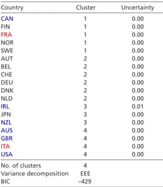
missal protection as the sole employment protection measure selected. All three unem- ployment measures – net unemployment replacement rates, generosity of benefits, and definition of suitable jobs – have been used in the cluster analysis.11 Table 3 displays the resulting country clusters. The BIC-maximizing MMBC algorithm chooses an ellipsoi- dal model with equal volume, shape, and orientation. It also identifies four clusters (and not two as with the VoC approach, or five as Figure 1 illustrates). Moreover, the country classifications do not mirror those of Iversen.
As an alternative to the heuristic classification from Figure1, we run the MMBC algo- rithm on the first principal component for unemployment protection and for employ- ment protection.12 The resulting clusters and their probability densities are displayed in 11 Interestingly, if all six of the original six measures are used in the cluster analysis, no clustering can be distinguished. We attribute this to the fact that we are estimating a model where k = 6 using only 21 cases.
12 Each of these principal components represents 60 and 69 percent of the variance for employ- ment and unemployment protection, respectively.
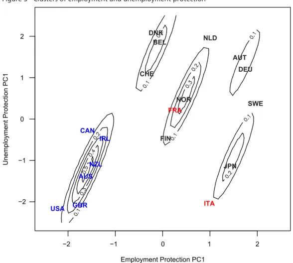
Figure 3 Clusters of employment and unemployment protection
Employment Protection PC1
Unemployment Protection PC1
−2 −1 0 1 2
−2
−1 0 1 2
AUS
AUT BEL
CAN
DNK
FIN FRA
DEU
IRL
ITA JPN NLD
NZL
NOR SWE
CHE
USA GBR
Note: Entries of the same color are classified in the same VoC category. Blue entries are LMEs, black are CMEs, and red entries are not classified or otherwise controversial.
Figure 3. While this analysis recovers the same major clusters as the visual method used in Iversen (2005) and Estévez-Abe, Iversen and Soskice (2001), some additional features are apparent. First, MMBC identifies five, not two, as the optimal number of clusters.
Second, the probability densities provide us with an assessment about how certain one is about the country clusters. While Australia and New Zealand are close to the peak of the densities and thus represent the core of the “occupational/general skill” profile, we are less certain about the placement of the Netherlands, Sweden, or even Austria and Germany in one particular cluster. Belgium, the Netherlands, and Sweden are assigned to different mini-clusters than what others researchers have identified. Third, the el- lipsoidal clusters that MMBC identifies are not possible under traditional clustering methods that are restricted to spherical cluster geometries.
Institutional complementarities in the macro-economy
In order to capture the theoretical core of the VoC argument, we now rely on the six in- dicators suggested by Hall and Gingerich (2004) to measure the institutional variation in corporate governance and in labor relations. We attempt to employ the same data as their study. This reduces the time period to one observation per country for 1990–1995 and, due to missingness on various indicators, fourteen countries (see Hall/Gingerich [2004: 11] for their data and sources). We concentrate on the MMBC analysis of the principal components (PCs) for the corporate governance and labor relations dimen- sions.13 The variable selection procedure chooses the first and third PC of corporate governance and the first PC of labor relations for the analysis. They explain about 65 and 66 percent of the total variance, respectively. Note that the third PC provides more 13 MMBC on the original six variables generates clusters highly dependent on G, the upper bound
for the number of clusters considered in model selection.
Table 4 Clusters of corporate governance and labor relations
Country Cluster Uncertainty
AUS 1 0.00
CAN 1 0.00
ESP 1 0.00
AUT 2 0.00
BEL 3 0.00
ITA 3 0.00
GBR 4 0.00
USA 4 0.00
DNK 5 0.00
FIN 6 0.00
FRA 6 0.00
SWE 6 0.00
DEU 7 0.00
PRT 7 0.00
No. of clusters 7
Variance decomposition EEE
BIC –40
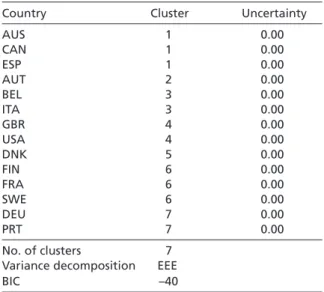
clustering information than the second one in this case. As Table 4 shows, the MMBC produces a classification of seven clusters. This result should be interpreted as a lack of structure in the data and indicates that countries cannot be grouped into LMEs and CMEs based on the operationalization of corporate governance and labor relations as employed by Hall and Gingerich (2004). In short, even for the core dimensions of pro- duction regimes, it is not possible to distinguish countries based on the quantitative indicators employed in the literature.
Data
For our dynamic analysis, we look to the extant literature on comparative capitalism to identify the variables purported to define the “three worlds” or VoC approaches. As mentioned above, there is an enormous number of dimensions along which countries vary, and several plausible measures for each dimension. Additionally, as the com- parative capitalism literature has grown, numerous idiosyncratic indices and coding schemes have emerged. As we are concerned with what the underlying data can tell us about clusters, we avoid constructed indices and, whenever possible, variables derived from expert coding. Since we are interested in both the classification of controversial cases and the assessment of the stability of clusters over time, we privilege the measures that provide some sort of time series and that maximize cross-sectional coverage.
It is clearly debatable what the proper indicators of welfare regimes and VoC are and whether some indicators represent constitutive features of a system or outcome vari- ables. We sidestep this theoretical discussion here and simply assume that previous re- search efforts have correctly identified some valid measurements of the two concepts. In our initial variable selection, we therefore rely only on measures that have been identi- fied by the initial theoretical literature, as well as the subsequent attempts to empirically identify country grouping as discussed above. In short, we rely on the previous judg- ment of scholarly work when identifying variables characterizing welfare production regimes and VoC. The model selection step in our MMBC algorithm then identifies those variables providing the most clustering information.
We are concerned with the actions of governments and economic actors, so we focus on political-economic institutional, policy, and structure variables. In addition, the fo- cus on time-series cross-sectional data and our reluctance to assume time-invariance of quantitative indicators obviously results in the omission of some variables that are claimed to be theoretically important. Among them are cross-shareholding measures, skill specificity, firm-bank relations, and inter-firm relations (e.g. measures of the den- sity of supply chains).
Missing data and our initial variable selection
Table 9 in the appendix presents the variables we have identified from the VoC and “three worlds” literature. Our data are characterized by a high degree of missingness, confound- ing the already thorny problem of classifying a relatively small number of countries ex- isting in a high-dimensional space. To get the most out of our analysis, we use multiple imputation techniques to generate ten complete datasets.14 We then break the data into three disjoint time slices: 1980–84, 1990–94, and 2000–03. We break the data up in this way for three reasons: first, focusing on fairly restricted time slices is consonant with the strong notions of equilibrium institutions and complementarity that underlie both the
“three worlds” and VoC approaches. Second, these windows are short enough to provide a snapshot but long enough to allow for some smoothing within the window. Finally, we allow for some time between slices, since institutions are purported to change slowly, if at all. Within each slice we take country averages for each variable. We therefore have 30 smaller datasets with 21 observations in each. We denote by dm,t the imputed data subset from imputation m = 1,…,10 at time slice t = {early, middle, late}.
There is currently no method to propagate the measurement uncertainty represented by the cross-imputation variation into a mixture model and model selection algorithm.
We attempt to make preliminary statements on clusters while also incorporating as much of the imputation-based uncertainty as possible. We recognize that our solution is suboptimal and discuss in the conclusion some ways in which future research might proceed in addressing this problem.
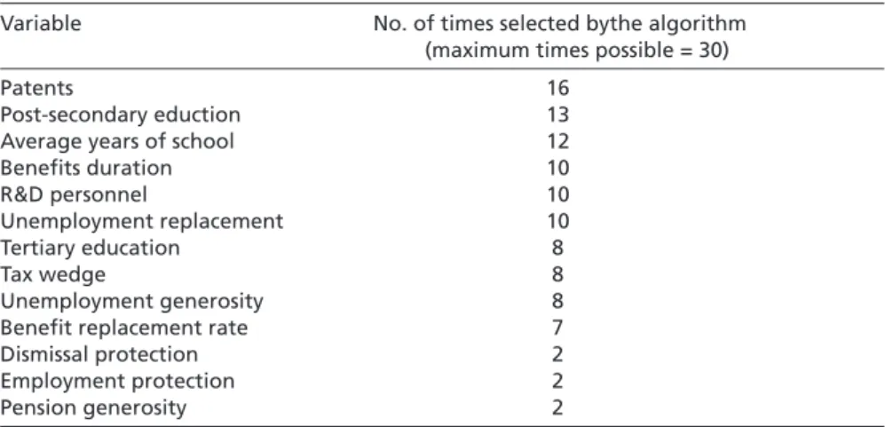
Specifically, we proceeded as follows: First, we conducted several exploratory variable- selection experiments across different dm,t to gather some idea as to what the most com- monly selected clustering variables are. We then attempted to select from among these variables a subset that had the lowest cross-imputation variation (relative to their means) and at the same time represented the major concepts from the VoC literature. The vari- ables selected here were percent of labor force with tertiary education, social security spending as %GDP, social insurance spending as %GDP, unemployment benefit generos- ity, pension generosity, unemployment replacement rate, restrictiveness of employment protection legislation, level of collective dismissal protection, proportion of those age 25 and over with post-secondary education, benefit replacement rate, benefit duration, the tax wedge, total R&D personnel per 1,000 people, and patents awarded per 1,000 people.
We then took these variables and performed the variable selection exercise across all the dm,t .
From the variable selection procedure, the following variables were selected most fre- quently (listed here in descending order of the frequency selected): social insurance spending as %GDP, post-secondary educational attainment, number of patents awarded 14 We used the R implementation of the Amelia software (Honaker/Blackwell/King 2006) for im-
putation.
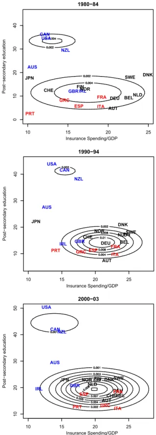
Figure 4 Clustering in two dimensions using the two most frequently selected variables across time and imputations. The cluster assignments vary over time and do not coincide with the VoC classications.
Note: Countries with the same color text are classified into the same VoC groups.
Insurance Spending/GDP
Post−secondary education
10 15 20 25
1020304050
2000−03
AUS
AUT BEL CAN
CHEDEU DNK ESP
FIN GBR FRA
GRC IRL
ITA JPN NORNLD NZL
PRT
SWE USA
Insurance Spending/GDP
Post−secondary education
10 15 20 25
10203040
1990−94
AUS
AUT BEL CAN
CHE DEU DNK
ESP
FIN GBR FRA
GRC IRL
ITA JPN
NOR NLD NZL
PRT
SWE USA
Insurance Spending/GDP
Post−secondary education
10 15 20 25
010203040
1980−84
AUS
AUT BEL CAN
CHE
DEU
DNK
ESP FIN GBR FRA GRC
IRL ITA JPN
NOR NLD NZL
PRT
SWE USA
per 1000 people, total R&D personnel per 1000 people, and pension generosity. The anal- ysis presented below is the result of clustering performed on three datasets (one for each time slice), each of which is composed of the mean values across all imputed datasets for that time slice. While we recognize that this throws away important information about the variability of these estimates, there is no readily available better method by which to proceed: Limiting our analysis to only the variables or countries for which complete data are available is not a preferable solution, especially when there are so few cases available.
Clustering with variable selection
Here we present four cluster analyses in which we gradually alter the variables under consideration. We begin with two baseline analyses. In the first, we use only the two most commonly identified variables in the cross-imputation investigation described in the previous section: social insurance spending as %GDP and post-secondary educa- tional attainment. In the second, we include the two variables mentioned and add to these patents, workers employed in basic R&D as proportion of the workforce, and pen- sion generosity. Again, these variables are selected because they provide “more informa- tion” on country clusters and not because they are especially pertinent theoretically.
When clustering in only two dimensions, results are most easily viewed graphically.
Figure 4 depicts contour plots describing the results across the three time periods. Text in the same color corresponds to the same VoC category.
Several things are immediately apparent. First, the number of clusters and the clustering solutions do not correspond to either the VoC or “three worlds” perspectives. While the United States, Canada, and New Zealand (LMEs all) are consistently grouped together, Great Britain and Ireland, also purported to be unambiguous LMEs, are at the core of the larger cluster that includes continental European economies for the early period.
Australia and Japan are ambiguously classified and move between groups over the time periods. As the contour lines indicate, the spread around the clusters is generally fairly small, but it is greater for the Canada-New Zealand-United States cluster and largest for the Australia-Japan mini-cluster.
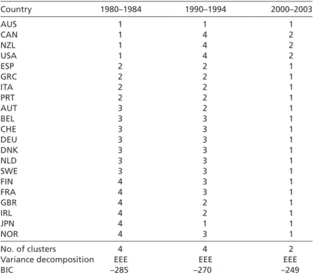
We extend the analysis by including more variables. Visualization becomes more dif- ficult in six dimensions, so we report the results in Table 5. These results are largely consistent with what we see in the two-variable case: Both the number of clusters and cluster membership change over time. The United States, Canada, and New Zealand continue to be grouped together, but Australia, Ireland, and Great Britain are lumped with other groups and change group affiliations.