Originally published as:
Kaveh Mollazade ; Mahmoud Omid ; Fardin Akhlaghian Tab ; Yousef Rezaei Kalaj ;
Seyed Saeid Mohtasebi ; Manueal Zude : Analysis of texture based features for predicting me- chanical properties of horticultural products by laser light backscattering imaging .
in: Computers and Electronics in Agriculture 98 (2013) 10 S. 34-45 DOI: 10.1016/j.compag.2013.07.011
1
Analysis of texture-based features for predicting
1
mechanical properties of horticultural products by
2
laser light backscattering imaging
3 4 5
Kaveh Mollazade a *, Mahmoud Omid a, Fardin Akhlaghian Tab b, Yousef Rezaei 6
Kalaj c, Sayed Saeid Mohtasebi a, Manuela Zude c 7
8
a Department of Agricultural Machinery Engineering, Faculty of Agricultural 9
Engineering and Technology, University of Tehran, P.O. Box 4111, Karaj 31587- 10
77871, Iran 11
b Department of Computer Engineering, Faculty of Engineering, University of 12
Kurdistan, Sanandaj, Iran 13
c Leibniz Institute for Agricultural Engineering Potsdam-Bornim (ATB), Max-Eyth- 14
Allee 100, 14469 Potsdam, Germany 15
16
* Corresponding author; Tel: +98 918 9720639; Fax: +98 261 2808138 17
E-mail address: mollazade@ut.ac.ir (K. Mollazade) 18
19 20 21
*Manuscript
Click here to view linked References
2 Abstract
22
Light backscattering imaging is an advanced technology applicable as a non- 23
destructive technique for monitoring quality of horticultural products. Because of 24
novelty of this technique, developed algorithms for processing this type of images are 25
in preliminary stage. Texture is one of the most important characteristics of images 26
and has been used widely in agro-food industry for assessing qualitative properties of 27
different types of products. The present study investigates the feasibility of texture- 28
based features to develop better models for predicting mechanical properties (fruit 29
flesh firmness or elastic modulus) of horticultural products. Images of apple, plum, 30
tomato, and mushroom were acquired using a backscattering imaging setup capturing 31
660 nm. After segmenting the backscattering regions of images by variable 32
thresholding technique, they were subjected to texture analyses and space domain 33
techniques in order to extract a number of features. Adaptive neuro-fuzzy inference 34
system models were developed for firmness or elasticity prediction using individual 35
types of feature sets and their combinations as input for prediction model applicable in 36
real-time applications. Results showed that fusion of the selected feature sets of image 37
texture analysis and space domain techniques provide an effective means for 38
improving the performance of backscattering imaging systems in predicting 39
mechanical properties of horticultural products. The maximum value of correlation 40
coefficient in the prediction stage was achieved as 0.887, 0.790, 0.919, and 0.896 for 41
apple, plum, tomato, and mushroom products, respectively.
42
Keywords: ANFIS, backscattering, feature fusion, quality evaluation, texture 43
analysis.
44 45
3 1. Introduction
46
Fruit flesh firmness and elastic modulus are two main mechanical parameters in 47
determining maturity and harvest time of horticultural products, and they are also key 48
parameters in evaluation and grading postharvest quality of fruit and some vegetables.
49
Mechanical properties of fresh produce change during growth and storage processes.
50
The conventional standard methods, like Magness-Taylor compression test and 51
Youngs’ modulus of elasticity, are not suitable for real-time applications, such as 52
grading and sorting machines, because the samples should be per definition or 53
potentially damaged during the test. Technical advances over the last few decades 54
considering spectrophotometers, multi- and hyperspectral systems as well as computer 55
vision systems have led to the development of non-destructive devices capable of 56
measuring internal qualitative parameters of horticultural products. Garcia-Ramos et 57
al. (2005) reviewed the non-destructive techniques developed to measure mechanical 58
properties of agricultural products. They concluded that optical techniques have the 59
advantage over the others, since they can estimate several internal variables, such as 60
sugar content, acid content, firmness, and elasticity, with a single sensor. However, it 61
has been shown that the application of spectroscopic analyses is not capable to build 62
robust calibrations for predicting the mechanical properties of the produce, while the 63
composition considering pigments, soluble solids content, dry matter, and moisture 64
content as well as the detection of internal physiological disorders appeared feasible 65
in several products (Zude, 2009).
66
As an optical technique, computer vision-based quality evaluation systems are being 67
used increasingly in the agro-food industry because of their rapid, non-contact, and 68
non-destructive manner as well as availability of inexpensive camera systems. Driven 69
4
by considerable improvements in imaging hardware and rapid progression in image 70
processing techniques, computer vision has established its applications for the internal 71
surveillance of both fresh and processed agro-food materials. In combination with 72
multi- or hyperspectral imaging more specific variation of the produce, such as the 73
detection of distribution of water core and internal browning has been shown.
74
Horticultural products, as biological materials, are supposed to be turbid and transmit 75
the light through the tissue depending on the wavelengths (Mireei, 2010). When light 76
source impinges to a biological tissue, its internal contents reflect most of the passing 77
light as scattering photons towards the exterior tissue surface. Due to physiochemical 78
properties of the tissue, photons are scattered at different angles, leading to their 79
stochastic interaction with the internal components of biological tissue like joint 80
surfaces of the cell wall, chloroplasts, mitochondria, etc (Nicolai et al., 2007).
81
Because of this interaction, backscattering photons carry information related to the 82
morphology and structures of the tissue, such as mechanical properties additionally to 83
the information on absorbing molecules. Few work groups showed that it is possible 84
to record backscattered photons by a camera equipped with an imaging sensor 85
sensitive in the range of visible and short wave near infrared (SWNIR) of 86
electromagnetic spectrum. The technique focuses on the processing of these types of 87
images and extracting knowledge from them has been named as backscattering 88
imaging. Based on the light source and imaging unit used, the technique is divided 89
into three categories: hyperspectral backscattering imaging (HBI), mutispectral 90
backscattering imaging (MBI), and laser light (monochromatic) backscattering 91
imaging (LLBI). The acquired images by these categories are similar, when we speak 92
about a certain wavelength (Mollazade et al., 2012a).
93
5
In most researches done to date, light intensity-based features in the space domain 94
were used to establish calibration models between the backscattering images and 95
reference physical properties. Qing et al. (2007) used the simplest type of features, i.e.
96
the area of backscattering region that is equal to the total number of pixels in the 97
segmented backscattering image, to predict firmness of apple. Another simple 98
technique is to use the mean intensity value (Qing et al., 2008) or some statistical 99
characteristics of pixels remained after segmenting the backscattering region (Noh 100
and Lu 2007). Lu (2004) introduced a method, known as radial averaging, in which 101
scattering region of photons is divided into several circular rings and then average 102
value of all pixels within each ring is recorded as the features of image. Using the 103
radial averaging approach, researchers applied different semi-Gaussian mathematical 104
functions, like exponential, Lorentzian, and Gompertz, to fit one-dimensional (1D) 105
scattering profiles as a function of distance. The values of parameters of the fitted 106
functions were then used as the features of images (Peng and Lu 2005, 2006, 2007).
107
Extracting the absorption and reduced scattering coefficients of 1D profile from the 108
Farrell’s diffusion theory model is another method used to predict firmness of apple 109
(Qin and Lu, 2006).
110
Although the above mentioned techniques have shown relatively fair utility in 111
describing the backscattering features, their relative performance in predicting 112
mechanical properties of horticultural products is not quite clear because they were 113
tested in separate studies, where the samples used were different and the experimental 114
setups were not the same. Hence, direct comparison of these feature extraction 115
techniques is required in order to investigate which method is the most suitable for 116
predicting mechanical properties of horticultural products. Furthermore, previous 117
techniques are based on some simple statistical features of pixel brightness or analysis 118
6
of 1D scattering profiles, and they did not investigate the pixel intensity pattern from 119
the overall two-dimensional (2D) scattering images acquired at a specific wavelength.
120
Use of 2D processing algorithms could present a chance to improve the performance 121
of backscattering imaging technique in predicting firmness and elasticity of 122
horticultural produce. Texture, as a 2D processing approach, is an important image 123
feature that corresponds to both brightness value and pixel locations. Many 124
researchers reported the feasibility of texture-based features in the food industry for 125
quality evaluation and inspection (Jackman and Sun, 2012). The distribution pattern 126
of backscattering photons is unique for each backscattering image, since the spatial 127
pattern in an image reflects the physiochemical properties of a product. Hence, by 128
utilizing the texture-based features, researchers may improve the accuracy 129
performance and take feasibility of backscattering systems in real-time applications.
130
Therefore, the overall objective of this research was to use LLBI technique for 131
predicting firmness and elastic modulus (elasticity) of a wide range of horticultural 132
products. The specific objectives were to:
133
Analysis the capability of different texture processing techniques for 134
firmness/elasticity prediction.
135
Compare the texture-based feature extraction techniques with those reported in 136
the previous researches (space domain techniques).
137
Establish intelligent models for firmness/elasticity prediction by adaptive 138
neuro-fuzzy inference system (ANFIS).
139
Suggesting the best feature set for real-time applications.
140 141
7 2. Materials and methods
142 143
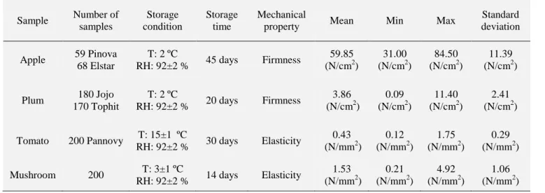
2.1. Data set 144
Mechanical properties obtained from two stony fruits (apple and plum), a non-stony 145
fruit (tomato), and a vegetable (mushroom) were used as data set. Harvested manually 146
from the garden and greenhouse, samples were visually inspected for appearance and 147
surface defects. Only those samples free of visual defects (such as scars, cuts, shrivel, 148
etc.) were selected for the experiments. To generate samples with variations in their 149
properties, they were separated into several groups and stored at the standard 150
temperature and relative humidity conditions. Groups of samples were withdrawn 151
from the storage chamber two hours before the experiments at regular intervals of 15, 152
3, 7, and 3 days for apple, plum, tomato, and mushroom, respectively. After 153
acquisition of backscattering images, samples were subjected to compression test.
154
Firmness was measured as the mechanical signature of stony fruits, while for tomato 155
and mushroom samples, elasticity was calculated (Mohsenin, 1986). Table 1 156
summarizes some information related to the samples, measurement conditions, and 157
mechanical tests.
158
Table 1.
159
2.2. Backscattering image acquisition 160
Backscattering images were acquired using an in-house built LLBI system (Baranyai 161
and Zude, 2009). The system mainly consisted of a wide dynamic range monochrome 162
CCD camera (JAI A50IR CCIR, JAI, Denmark) with a zoom lens (model H6Z810, 163
PENTAX Europe GmbH, Germany), a solid-state laser diode emitting at 660 nm as 164
the light source (LPM series, Newport Corp., USA), a laser driver, a sample holder 165
unit, video converter (VRM AVC-1, Stemmer Imaging GmbH, Germany), and a 166
8
computer equipped with an in-house developed software to acquire the backscattering 167
images. The backscattering images with the spatial resolution of 720×576 pixels were 168
acquired in a dark room and laser diode spot of 1 mm diameter provided an acceptable 169
signal to noise ratio. The camera was placed perpendicular to the sample holder while 170
the incident angle of the laser beam was adjusted to 15º.
171 172
2.3. Image processing 173
Image processing was carried out using MATLAB R2009a and its image processing 174
toolbox (The Mathworks, Inc., Natick, MA, USA).
175 176
2.3.1. Segmentation 177
Segmentation plays a key role in processing of backscattering images. If it does not 178
perform well, useful information may be omitted. Segmentation operation consists of 179
segregating the region of interest (ROI), backscattering photons minus those saturate 180
the CCD of camera, from the background. This operation was carried out in two steps 181
as following:
182
1. Removing saturated pixels: Since saturated region in images consists of photons 183
that directly return to the camera’s sensor, the light intensity of pixels in this region is 184
close to its maximum value, i.e. 255. By a trial and error procedure, it was found that 185
saturated regions are segmented successfully by the static threshold value of 252.
186
2. Segmenting regions consists of backscattering photons from the background:
187
Variable thresholding by local statistics is a powerful segmentation technique when 188
background illumination is uneven. At each pixel of image, the threshold value is 189
defined based on some statistical features extracted from the neighborhood pixels 190
(Gonzalez and Woods, 2004). In the current study, threshold values were selected 191
9
based on the standard deviation and the average of a 3×3 neighborhood for each pixel.
192
These features were very useful in setting local thresholds, because they are contrast 193
and average of local intensity.
194 195
2.3.2. Texture analysis 196
A wide variety of techniques have been proposed for describing image texture (Zheng 197
et al., 2006). Approaches to texture analysis are usually classified into four categories:
198
statistical, structural, transform-based, and model-based. Statistical techniques 199
represent the texture indirectly by non-deterministic properties that govern the 200
distribution and relationship between the grey levels of an image. Structural 201
approaches represent texture through some structural primitives constructed from grey 202
values of pixels. In the transform methods of texture analysis, an image is represented 203
in a space whose co-ordinate system has an interpretation that is closely related to the 204
characteristics of a texture (such as frequency or size). Model-based texture analysis 205
attempts to interpret an image texture by use of, respectively, generative image model 206
and stochastic model. The parameters of the model are calculated, based on the 207
relationship of the grey values between a pixel and its neighboring pixels, and then 208
these are used for image analysis.
209
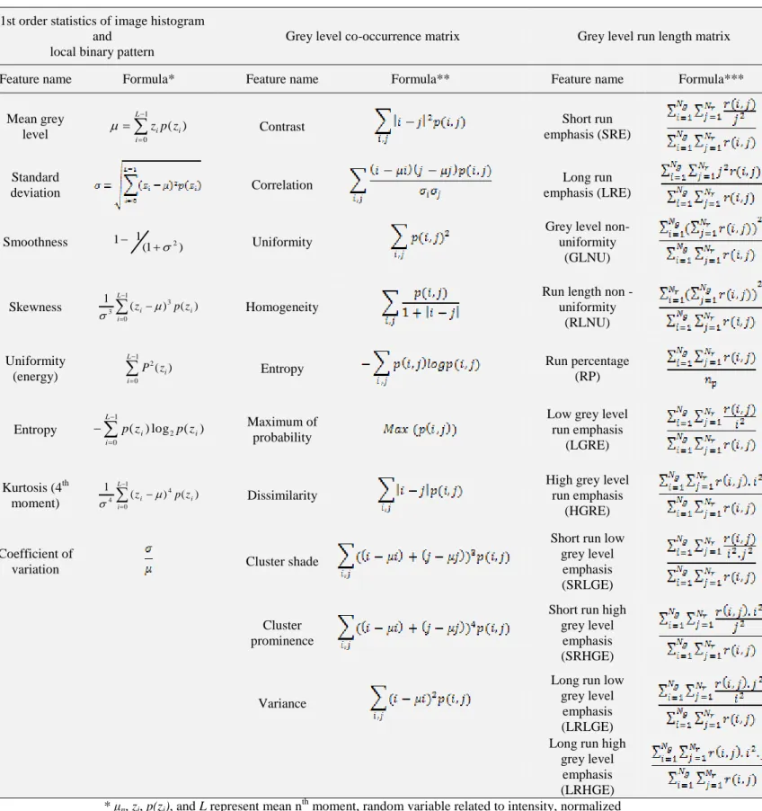
To process backscattering images, texture-based features from four statistical 210
techniques (first order statistics of image histogram (FOSH), grey level co-occurrence 211
matrix(GLCM), grey level run length matrix (GLRLM), and local binary pattern 212
(LBP)), three transform-based techniques (wavelet transform, Gabor transform, and 213
Tamura), and two model-based techniques (fractal model and simultaneous 214
autoregressive model), were considered. Structural techniques were not considered in 215
this research since the structural primitives used in these methods can only describe 216
10
very regular textures (Bharati et. al.,2004). Furthermore, structural techniques are 217
rarely used in the food industry to describe texture characteristics (Zheng et al., 2006).
218
A brief description of these techniques is provided in the following subsections.
219 220
2.3.2.1. First order statistics of image histogram 221
First order statistics of image histogram are considered as the most basic feature 222
extraction method of image texture. They act based on the probability of occurring 223
pixel intensity values in the image. They depend only on individual pixel values and 224
not on interaction of neighboring pixel values. First the histogram of grey level 225
backscattering images was extracted. The histograms were then normalized according 226
to the following formula:
227
(1) 228
where H(zi) is the image histogram, p(zi) is the normalized histogram, and NI is the 229
total number of arrays in the image matrix. Using the normalized histogram and 230
relations based on the occurrence of grey levels, eight statistical features were 231
extracted from each backscattering image (Bevk and Kononenko, 2002). The list of 232
features is presented in Table 2.
233 234
2.3.2.2. Grey level co-occurrence matrix 235
A GLCM is a matrix in which grey level pixels are considered in pairs with a relative 236
distance d and orientation θ among them. The entry Gdθ (i, j) of this matrix is the 237
number of occurrences of a pair of grey levels, i and j, for the specified displacement.
238
The scattering images were analyzed using the distance d=1 pixel with angles θ = 0, 239
45, 90, and 135º as suggested by Haralick (1979). After calculating GLCMs, they 240
were normalized so that sum of arrays in the normalized matrix is equal to 1. Ten 241
11
features were then extracted from each normalized GLCM according to Table 2 242
(Haralick et al., 1973). Thus, a total of 40 features (4 orientations × 10 statistical 243
features) were extracted from each image.
244 245
2.3.2.3. Grey level run length matrix 246
Run length technique records the coarseness of a texture in specified directions by 247
encoding textural information based on the number each grey level appearing in the 248
image by itself. A run is defined as a string of consecutive pixels which have the 249
same grey level intensity along a specific linear orientation. Fine textures tend to 250
contain more short runs with similar grey level intensities, while coarse textures have 251
more long runs with significantly different grey level intensities. A GLRLM is a 252
matrix in which each element r(i,j) determines the total number of occurrence of run 253
lengths j in the grey level i in specified direction θ. Run length matrices at four 254
directions θ = 0, 45, 90, and 135º were extracted for each backscattering image. Once 255
the GLRLMs were calculated along each direction, 11 texture descriptors, as 256
suggested by Tang (1998), were calculated to capture the texture properties and 257
differentiate among different textures (Table 2). For each image, a total of 44 features 258
(11 GLRLM texture descriptors × 4 directions) were obtained.
259 260
2.3.2.4. Local binary pattern 261
The LBP texture analysis operator is defined as a grey-scale invariant texture 262
measure, derived from a general definition of texture in a local neighborhood. For 263
each pixel in an image, a neighborhood of the image (usually a 3 × 3 window) is 264
considered and the intensity value of neighboring pixels is compared with that of the 265
central pixel. If the intensity value of neighboring pixels is greater or equal to the 266
12
central pixel value, they are replaced with ones. Otherwise, their value is zero.
267
Finally, central pixel is replaced with the binary weighted sum of neighboring pixels 268
and the neighboring window is transferred to the next pixel. The output of LBP 269
operator is a P-bit binary number (P is the number of neighboring pixels), which can 270
take 2P different values. Furthermore, LBP is completely dependent to indexing of 271
pixels contained in the neighborhood. Thus, in order to assign a unique value to each 272
private binary pattern, LBP matrices were robust to rotation by clockwise rotation of 273
the obtained binary number and selecting the maximum possible value (Ojala et al., 274
2002). Finally, 8 statistical features were extracted from the normalized histogram of 275
GLRLM of each backscattering image.
276 277
2.3.2.5. Wavelet transform 278
Wavelet transform is a useful tool for analyzing the texture of agricultural materials.
279
A discrete wavelet transform (DWT) decomposes an image onto multiple wavelet 280
components using a filter bank as suggested by Mallat (1989). It provides four sets of 281
coefficient at each level of decomposition. Rows of the input image are first passed 282
through the low and high pass filters, followed by down-sampling along the rows by a 283
factor of 2. The columns of resulting images from both filters are sent through low 284
and high pass filters followed by down sampling along the columns to obtain four sets 285
of coefficients; namely, approximation, horizontal, vertical, and diagonal details 286
(Choudhary et al., 2008). Backscattering images were subjected to six levels of 287
wavelet decomposition using a fourth-order Daubechies mother wavelet (Db4), which 288
is the most popular mother wavelet family for image texture analysis. At each level of 289
decomposition, approximation coefficients and wavelet detail coefficients were 290
obtained for horizontal, vertical, and diagonal orientations. To determine optimum 291
13
level of decomposition, backscattering images at each level of decomposition were 292
compared to the original images. As is shown in the Figure 1, an increase in the levels 293
of decomposition leads to increase the amount of down-sampling, resulting in lower 294
resolutions at successive levels. So, the wavelet coefficients from first to the fourth 295
level of decomposition were considered to be used in feature extraction stage. Four 296
statistical descriptors including mean, standard deviation, energy, and entropy were 297
extracted from each level of decomposition. A total of 64 features (4 statistical 298
descriptors × 4 wavelet coefficients × 4 decomposition levels) were obtained from the 299
DWT of each backscattering image.
300 301
2.3.2.6. Gabor transform 302
Gabor transform is one of the most effective and most popular filter-based approaches 303
to extract texture features of an image. Gabor filter is obtained by multiplying a 304
Gaussian function in a directional sine function. Therefore, this filter generates 305
powerful responses at locations with specific local direction and frequency (Zhu et al., 306
2007). Gabor wavelet is a kind of wavelet transform function in which its mother 307
wavelet is a Gabor filter. After applying the Gabor wavelet on backscattering images, 308
a new matrix with M×N dimension was obtained. Each dimension represents a 309
frequency in a specific direction. Since each element of the final image, after applying 310
the Gabor transform, is a complex number with both real and imaginary parts, the 311
matrix magnitude was used for feature extraction (Figure 2). Mean, standard 312
deviation, energy, and entropy were used as statistical descriptors in order to build the 313
feature vector containing the texture descriptors of backscattering images by Gabor 314
filter. These statistical operators were then applied on the magnitude of matrices 315
found in the previous section for each backscattering image in four frequencies 316
14
(0.1768, 0.25, 0.3536, and 0.5 Hz) and four directions (0, /4, /2, and 3 /4 radian).
317
The size of feature vector based on the Gabor transform was 64 (4 statistical 318
descriptors × 4 frequencies × 4 directions).
319 320
2.3.2.7. Tamura 321
Tamura features are designed based on psychological studies on human visual 322
perception of objects texture (Tamura et al., 1978). These features include coarseness, 323
contrast, directionality, line-likeness, regularity, and roughness. Since the last three 324
features are derived from the first three ones, only coarseness, contrast, and 325
directionality just were extracted from each backscattering image.
326 327
An image contains textures at several scales; coarseness aims to identify the largest 328
size at which a texture exists, even though a smaller micro texture may exist. To 329
compute the coarseness, using a 2k ×2k (k=0,1,…,5) window, first a moving average 330
filter Ak(x,y) was applied on each pixel:
331
(2) 332
where g(i,j) is the intensity value at pixel (i,j).
333
Then at each pixel differences between pairs of Ak(x,y) corresponding to non- 334
overlapping neighborhoods on opposite sides of the point in both horizontal and 335
vertical orientations were calculated:
336
(3) 337
(4) 338
In order to determine the filter window size for each pixel which gives the highest 339
output value, the value of k was taken in which E is maximized in either direction.
340
The coarseness was then computed by the following formula:
341
15
(5) 342
Contrast aims to capture the dynamic range of grey levels in an image, together with 343
the polarization of the distribution of black and white. The first is measured using the 344
standard deviation of grey levels ( ) and the second from the kurtosis α4. The contrast 345
measure was therefore defined as:
346
(6) 347
Directionality is a measure of the orientation of the image grey values. To compute 348
the directionality, initially two simple masks were used first to detect edges in 349
backscattering images. At each pixel the angle and magnitude were calculated. A 350
histogram of edge probabilities was then built up by counting all points with 351
magnitude greater than a threshold and quantizing by the edge angle. The histogram 352
reflects the degree of directionality. Finally, the directionality was then computed 353
from the sharpness of the peaks of histogram using their second moments.
354 355
2.3.2.8. Fractal model 356
In the image analysis of agro-food materials, fractal dimension can be used to 357
estimate and quantify the complexity of the shape or texture of images. The fractal 358
dimension gives a measure of the roughness of an image. Intuitively, the larger the 359
fractal dimension, the rougher the texture is (Zheng et al., 2006). There are a number 360
of methods proposed for defining the fractal dimensions, where the most common one 361
is the Hausdorff’s dimension (D0):
362
(7) 363
where N(ε) is the number of hypercubes of Euclidean dimension E, and length ε that 364
fill the object. In this research, a new developed algorithm known as segmentation- 365
16
based fractal texture analysis (SFTA) was used to extract the Hausdorff’s fractal 366
dimension of backscattering images (Costa et al., 2012). The SFTA algorithm was 367
implemented in two steps. In the first step, a set of threshold values was computed 368
using multi-level Otsu algorithm and distribution of grey levels in the input images.
369
The number of optimum thresholds was set to 8, as suggested by Costa et al. (2012).
370
After that, the grey level backscattering images were disintegrated into a set of binary 371
images by selecting pairs of thresholds from the threshold set and applying the two- 372
threshold binary decomposition (TTBD) algorithm. The number of resulting binary 373
images was 16. Figure 3 illustrates the decomposition of a backscattering image taken 374
from a tomato sample at 660 nm using the TTBD algorithm. The threshold set for this 375
sample was as T=[0, 0.0039, 0.0391, 0.1367, 0.2188, 0.3477, 0.4961, 0.6914]. In the 376
second step of SFTA, Hausdorff’s dimension was computed from the borders of each 377
binary image by applying the box counting algorithm (BCA). In the BCA, binary 378
images were divided into a grid composed of squares of size ε×ε. The number (N(ε)) 379
of squares of size ε×ε that contains at least one pixel of ROI was counted. A log N(ε) 380
versus log ε-1 curve was drawn for each binary image by varying the value ε. The 381
curve was approximated by a straight line using the least squares fitting approach.
382
Then, the slop of this line was recorded as the Hausdorff’s dimension of each binary 383
image. The size of fractal feature vector for each backscattering image was 16 (Figure 384
3).
385 386
2.3.2.9. Autoregressive model 387
Simultaneous autoregressive (SAR), as a model-based texture analysis technique, has 388
found many applications in image segmentation (Sukissian, 1994, Sukissian et al., 389
1997). This model acts based on the spatial relationship between the pixels of an 390
17
image. It assumes that intensity of pixels is the weighted sum of intensity from the 391
neighboring pixels. In fact a SAR models the relationship between a pixel and its 392
neighboring pixels using the following linear combination (Jain, 1989):
393
(8) 394
where f(s), f(q), μ, ε(q), N, and θ(q) are image intensity at position s, image intensity at 395
position q, bias value, noise value, number of neighboring pixels, and model 396
parameters, respectively. In the current research, the bias value was adjusted to the 397
average of light intensity of entire image, which was formerly normalized between 0 398
and 1. A Gaussian random variable with mean zero and variance σ2 was used to adjust 399
the noise value. The number of neighboring pixels considered was equal to four 400
according to the pattern shown in Figure 4. For each backscattering image, a total of 401
five SAR model features, including values of θ in four neighboring pixels together 402
with the minimum prediction error variance, were extracted.
403
Table 2 404
Figure 1 405
Figure 2 406
Figure 3 407
Figure 4 408
409
2.3.3. Space domain analysis 410
In order to assess the effectiveness of texture analysis techniques, backscattering 411
images were subjected to several space domain techniques proposed by researchers in 412
literature. These techniques as described in the ―Introduction‖ section, were:
413
1. Total number of pixels in the segmented backscattering region of image, 414
18
2. Statistical features of segmented backscattering region of image (mean, min, 415
max, sum, standard deviation, and variance), 416
3. Radial averaging technique (25 rings with thickness of five pixels), 417
4. Modified Lorentzian function parameters (four parameters: a, b, c, and d), 418
5. Modified Gompertz function parameters (four parameters: α, β, ε, and δ), and 419
6. Farrell’s diffusion theory model parameters (two parameters: absorption (µa) 420
and reduced scattering coefficients (μs')).
421
Readers can refer to the references provided in the ―Introduction‖ section to get more 422
information about these techniques.
423 424
2.4. Adaptive neuro-fuzzy inference system (ANFIS) 425
A neuro-fuzzy system integrates the advantages of artificial neural networks (ANNs) 426
with rule-based fuzzy inference systems (FIS). It covers the lacks of these techniques 427
when they are used individually. ANNs are efficient structures capable of learning 428
from examples, while fuzzy systems are suitable for uncertain knowledge 429
representation. These hybrid technique brings learning capability of ANN to FIS.
430
During the learning process, a number of desired input–output data pairs are used, and 431
then parameters associated with the membership functions and rules of a Takagi- 432
Sugeno type FIS are tuned by ANN so as to map the inputs to outputs. The 433
computation and adjustment of these parameters is facilitated by a gradient vector, 434
which provides a measure of how well the FIS is modeling the input/output data for a 435
given set of parameters. From the topology point of view, ANFIS is an 436
implementation of a representative FIS using a feed forward neural network-like 437
structure (Jang, 1993).
438
19
The fuzzy logic toolbox of MATLAB R2009a was used to create ANFIS models (The 439
Mathworks, Inc., Natick, MA, USA). The inputs to the models were the normalized 440
feature sets (in the range 0 to 1) extracted from backscattering images, while the 441
output was the firmness or elasticity of samples. ANFIS is susceptible to the curse of 442
dimensionality when number of inputs exceeds three. The training time increases 443
exponentially with respect to the number of fuzzy sets per input variable used. An 444
effective procedure to reduce the dimension of the input vector is to use principal 445
component analysis (PCA). The technique was outlined by authors previously (Omid 446
et al., 2009 and 2010). Hence, the inputs were subjected to the PCA and only the first 447
three principal components were fed to the ANFIS. The performance of ANFIS is 448
highly dependent to its structure. Therefore, four significant adjustments were made in 449
the structure of ANFIS models in order to find best one for predicting 450
firmness/elasticity of horticultural produce. Settings include the number of 451
membership functions (changed from 2 to 5 with step size of 1), types of input 452
membership functions (triangular, trapezoidal, bell-shaped, Gaussian, and sigmoid), 453
types of output membership function (constant and linear), and optimization methods 454
(hybrid and back-propagation). Each ANFIS model with its specific setting was run 455
20 times and the best was defined as the one with the best overall statistical accuracy 456
measures.
457 458
2.5. Statistical measures 459
To ensure the models were not over-fitted and the prediction results truly represent the 460
model performance, the samples were first divided into three separate parts randomly.
461
The first part (or 60% of all samples) was used for training, 15% of all samples were 462
used for cross-validation, and the remaining samples were used for independent test or 463
20
prediction. Calibration models for firmness and elasticity were developed using 464
ANFIS from the training samples. Cross-validation was used to supervise the training 465
process in order to prevent the over-training. Thereafter, the calibration models were 466
used to predict the independent part of samples. The models were evaluated using root 467
mean squares errors for cross validation (RMSECV) and prediction (RMSEP).
468
(9) 469
where is the actual value, yi is the predicted value, and n is the number of samples 470
in prediction or calibration stages. In addition, correlation coefficients for calibration 471
(Rc) and prediction (Rp) were also calculated. Processing time is an important factor 472
when we want to use a backscattering imaging system in real-time applications. For 473
each feature extraction technique, the processing time was recorded to be used as an 474
evaluation criterion. MATLAB codes were implemented and run in a laptop computer 475
with this configuration: Core 2Duo CPU, 2.53 GHz, 4 GB RAM, Windows 7 OC 476
configuration.
477 478
3. Results and discussion 479
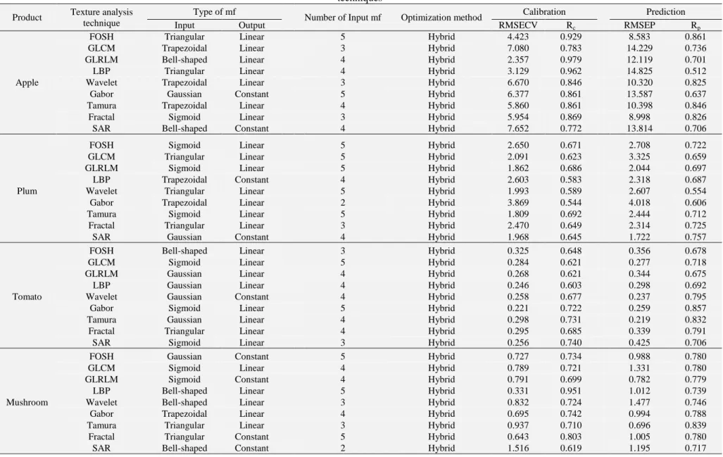
3.1. Individual feature set models 480
The statistical measures of individual texture-based feature models for predicting 481
firmness/elasticity of apple, plum, tomato, and mushroom by ANFIS are presented in 482
Table 3. The best firmness prediction of FOSH technique using ANFIS for apple was 483
the highest (Rp=0.861) followed by the Tamura (Rp=0.846)), fractal (Rp=0.826)), and 484
wavelet (Rp=0.825)). The highest prediction accuracies for plum, tomato, and 485
mushroom were obtained by the SAR (Rp=0.757), Gabor (Rp=0.857), and Tamura 486
(Rp=0.839), respectively, whereas, for the same, the wavelet (Rp=0.554), GLRLM 487
(Rp=0.675), and SAR (Rp=0.717) produced the lowest prediction performance.
488
21
Comparing to the other texture analysis techniques, Tamura and fractal provided good 489
results for all samples leading to select them as the best texture-based techniques for 490
analysis of backscattering images because of their consistency in firmness/elasticity 491
prediction performance. This reflects the fact that border of segmented regions along 492
with distribution pattern of light intensity in backscattering images are closely related 493
to the mechanical properties of horticultural products. On the other hand, LBP in all 494
cases was one of four techniques showed the lowest correlation with the 495
firmness/elasticity changes. The poor performance of LBP features can be attributed 496
to the small changes of run length values in backscattering images when mechanical 497
properties of products change. Comparing the results obtained for apple, plum, 498
tomato, and mushroom show that Tamura, fractal, FOSH, and GLCM are the best 499
texture analysis methods in overall for predicting firmness/elasticity of horticultural 500
produces when they are used as an individual feature set.
501
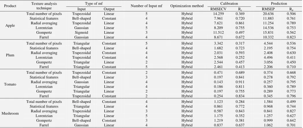
Regarding the space domain features (see Table 4), results showed that statistical, 502
radial averaging, and Farrell’s features have the highest performance in predicting 503
firmness/elasticity of apple, plum, tomato, and mushroom compared to the other 504
techniques. However, for all products, the lowest prediction performance was 505
recorded for the total number of pixels technique. Lorentizan and Gompertz 506
techniques did not show the consistency in firmness/elasticity prediction so that they 507
presented acceptable performance for tomato fruit, while for the plum and mushroom 508
the accuracy of these techniques was considerably low. The reason for this is that the 509
area of backscattering region for tomato fruit was bigger than that of mushroom and 510
plum resulting in the better fitness of 1D backscattering profile by Lorentzian and 511
Gomperzt functions. Comparing the results obtained in the Tables 3 and 4 512
demonstrates texture analysis techniques provide better performance than that of 513
22
space domain techniques when they are used individually. However, the differences 514
are very small.
515
Table 3 516
Table 4 517
3.2. Real-time feature set models 518
In real-time applications, such as grading/sorting machines, two factors are important:
519
prediction accuracy and processing time. To compare the capability of different 520
texture and space domain techniques for real-time applications, processing time 521
during implementation and feature extraction process for each technique was 522
recorded. Figures 5 and 6 illustrate, respectively, the time achieved by various texture 523
and space domain methods on the study data set, respectively. Results show that the 524
type of sample has no significant impact on the processing time because the image 525
dimensions are the same. Obviously, Tamura, fractal, Gabor, and GLRLM are 526
unsuitable for real-time systems since they require considerable much time for 527
implementation. On the other hand, FOSH, GLCM, LBP, wavelet, and SAR were the 528
fastest techniques because their processing time was less than 0.5 second. Space 529
domain techniques, except radial averaging, recognized to be suitable for real-time 530
purposes since they need processing time lower than that of our threshold, i.e. 0.5 531
second.
532
Many researchers reported that the combined feature models perform better than 533
individual models. Hence, all of the real-time features were combined together to 534
make two data sets, one for texture analysis methods and the other for space domain 535
techniques. The combination process leads to produce data sets with large number of 536
inputs so that the size of new texture analysis and space domain feature vectors was 537
125 (8 FOSH + 40 GLCM + 8 LBP + 64 wavelet + 5 SAR) and 17 (2 Farrell + 4 538
23
Lorentzian + 4 Gompertz + 6 statistical features + 1 Total number of pixels), 539
respectively. The large number of model inputs may leads to increase the execution 540
time and reduce the predictive accuracy. Using feature selection approaches such as 541
PCA, sensitivity analysis, genetic algorithms (GA), etc., these problems go away by 542
eliminating redundant features. In this study, genetic algorithm technique (GA) was 543
used for feature reduction as many researchers reported its suitability for this aim 544
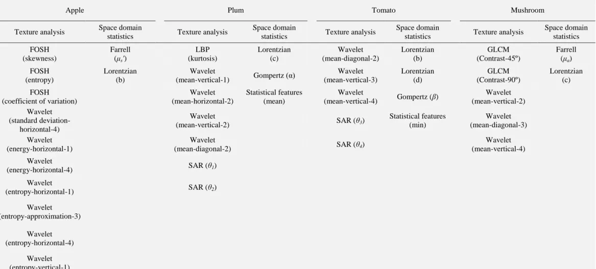
(Leardi, 2000; Mollazade et al., 2012b). Table 5 shows the list of top texture analysis 545
and space domain features obtained by GA for apple, plum, tomato and mushroom.
546
Feature selection process considerably reduced the size of feature vectors so that the 547
size of texture analysis and time domain feature vectors was 10 and 2 for apple, 7 and 548
3 for plum, 5 and 4 for tomato, and 5 and 2 for mushroom, respectively. The wavelet 549
and modified Lorentzian function are superior compared to others since most of the 550
top features have been selected from the features of these techniques.
551
The ANFIS model with the selected texture analysis features gave the prediction 552
correlation coefficient of 0.872, 0.776, 0.853, and 0.827 for apple, plum, tomato, and 553
mushroom, respectively, which are slightly higher than that obtained by the ANFIS 554
models with individual texture analysis techniques (Tables 3 and 6). Regarding the 555
selected real-time space domain features, the same behavior has been observed so that 556
prediction correlation coefficient for apple, plum, tomato, and mushroom showed an 557
increase from 0.823 to 0.847, 0.754 to 0.762, 0.796 to 0.864, and 0.744 to 0.764, 558
respectively (Tables 4 and 7).
559 560
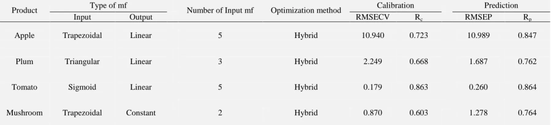
3.3. Fusion of selected real-time feature sets model 561
The real-time features selected from texture analysis and space domain techniques 562
(Table 5) were combined together in order to make a single feature set having the 563
24
benefits of two feature sets. Figure 7 presents the statistical measures of combined 564
feature set model by ANFIS. Using the combined feature set model, the prediction 565
accuracies of all the products were improved in comparison to the single real-time 566
selected feature set models (Tables 6 and 7, and Figure 7). The correlation coefficient 567
in prediction stage for tomato was highest (Rp=0.919) followed by mushroom 568
(Rp=0.896), apple (Rp=0.887), and plum (Rp=0.790). This indicates that the integration 569
of space domain and texture-based features considerably improved firmness/elasticity 570
prediction for tomato and mushroom products but with a lesser degree of accuracy for 571
apple and plum fruits. With the proposed features for laser induced backscattering 572
imaging, the system is suitable to be implemented as a non-destructive technique in 573
real-time machines to grade/sort horticultural products based on their mechanical 574
properties. More efforts are needed to improve the capabilities of this system to meet 575
the real-time requirements for monitoring different qualitative properties of 576
horticultural produce. Works in this direction is in progress by authors.
577
Figure 5 578
Figure 6 579
Table 5 580
Table 6 581
Table 7 582
Figure 7 583
4. Conclusions 584
In this research an experimental analysis of a number of different texture analysis 585
methods along with several space domain techniques was carried out for predicting 586
mechanical properties of apple, plum, tomato and mushroom. Calibration models 587
were developed by ANFIS that is an efficient artificial intelligent approach for 588
25
modeling. Texture analysis methods showed slightly better results than those of the 589
space domain techniques when feature set of each technique was fed independently to 590
the ANFIS. Results showed that combination of real-time features of texture analysis 591
techniques was more effective than when they were used individually for predicting 592
firmness/elasticity. Similar results were observed for the space domain techniques too.
593
Feature selection process showed that not only it leads to a considerable reduction in 594
the feature vectors but also improves the prediction accuracy of ANFIS models.
595
Among all of the techniques used for feature extraction, wavelet transform and 596
modified Lorentzian function are introduced as the best techniques for analysis of 597
backscattering images. For all horticultural products in this research, it was found that 598
integrating selected real-time features of both texture analysis and space domain 599
techniques provides the best prediction results. The statistical performance for apple, 600
tomato, and mushroom was in an acceptable range while real-time sensing of firmness 601
for plum fruit was still poor. Future works should focus on the improving the accuracy 602
and robustness of methods described in this research by applying the correction of 603
light scattering distortion algorithms and methods that lead to increase signal to noise 604
ratio.
605 606
Acknowledgments 607
The authors are grateful for the financial and technical support received from 608
University of Tehran, University of Kurdistan, and Leibniz Institute for Agricultural 609
Engineering Potsdam-Bornim (ATB) for this project.
610 611
References 612
26
Baranyai, L., Zude, M., 2009. Analysis of laser light propagation in kiwi fruit using 613
backscattering imaging and Monte Carlo simulation. Comput. Electron. Agric.
614
69, 33–39.
615
Bevk, M., Kononenko, I., 2002. A statistical approach to texture description of 616
medical images: A preliminary study. Proceedings of the 15th IEEE Symposium 617
on Computer-Based Medical Systems (CBMS 2002), 239-244.
618
Bharati, M.H., Liu, J.J., MacGregor, J.F., 2004. Image texture analysis: methods and 619
comparisons. Chemometr. Intell. Lab. 72, 57–71.
620
Choudhary, R., Paliwal, J., Jayas, D. S., 2008. Classification of cereal grains using 621
wavelet, morphological, colour, and textural features of non-touching kernel 622
images. Biosyst. eng. 99, 330-337.
623
Costa, A.F., Humpire-Mamani, G.E., Traina, A.J.M., 2012. An efficient algorithm for 624
fractal analysis of textures. In SIBGRAPI 2012: XXV Conference on Graphics, 625
Patterns, and Images, 39-46.
626
Garcia-Ramos, F.J., Valero, C., Homer, I., Ortiz-Canavate, J., Ruiz-Altisent, M., 627
2005. Non-destructive fruit firmness sensors: a review. Span. J. Agric. Res. 3(1), 628
61-73.
629
Gonzalez, R.C., Woods, R.E., Eddins, S.L., 2004. Digital Image Processing using 630
MATLAB. Pearson Prentice Hall, New Jersey, USA.
631
Haralick, R.M., 1979. Statistical and structural approaches to texture. P. IEEE. 67, 632
786–804.
633
Haralick, R.M., Shanmugam, K., Dinstein, I., 1973. Textural features for image 634
classification. IEEE. T. Syst. Man. Cyb. 6, 610–621.
635
Jackman, P., Sun, D.W., 2012. Recent advances in image processing using image 636
texture features for food quality assessment. Tr. Food. Sci. Tec. 29(1), 35-43.
637
27
Jain, A., 1989. Fundamentals of Digital Image Processing. Prentice Hall International, 638
Englewood Cliffs, USA.
639
Jang, J.S.R., 1993. ANFIS: adaptive-network-based fuzzy inference system. IEEE. T.
640
Syst. Man. Cyb. 23(3), 665-685.
641
Leardi, R., 2000. Application of genetic algorithm-PLS for feature selection in 642
spectral data set. J. Chemometr. 14, 643-655.
643
Lu, R., 2004. Multispectral imaging for predicting firmness and soluble solids content 644
of apple fruit. Postharvest. Biol. Tec. 31, 147–157.
645
Mallat, S.G., 1989. A theory for multiresolution signal decomposition: the wavelet 646
representation. IEEE. T. Pattern. Anal. 11(7), 674-693.
647
Mireei, S.A., 2010. Nondestructive Determination of Effective Parameters on 648
Maturity of Mozafati and Shahani Date Fruits by NIR Spectroscopy Technique.
649
PhD Dissertation. Department of Mechanical Engineering of Agricultural 650
Machinery. University of Tehran. Iran. In Persian.
651
Mohsenin, N.N., 1986. Physical Properties of Plant and Animal Materials, Second 652
Edition Revised. Gordon and Breach Science, NY, USA.
653
Mollazade, K., Omid, M., Akhlaghian Tab, F., Mohtasebi, S.S. 2012a. Principles and 654
applications of light backscattering imaging in quality evaluation of agro-food 655
products: a review. Food. Bioprocess. Tech. 5(5), 1465-1485.
656
Mollazade, K., Omid, M., Akhlaghian Tab, F., Mohtasebi, S. S., Zude, M., 2012b.
657
Spatial mapping of moisture content in tomato fruits using hyperspectral imaging 658
and artificial neural networks. 4th International Workshop on Computer Image 659
Analysis in Agriculture, 09 - 11 July, Valencia, Spain.
660
28
Nicolai, B.M., Beullens, K., Bobelyn, E., Peirs, A., Saeys, W., Theron, K.I., 661
Lammertyn, J., 2007. Nondestructive measurement of fruit and vegetable quality 662
by means of NIR spectroscopy: a review. Postharvest. Biol. Tec. 46, 99-118.
663
Noh, H.K., Lu, R., 2007. Hyperspectral laser-induced fluorescence imaging for 664
assessing apple fruit quality. Postharvest. Biol. Tec. 43, 193–201.
665
Ojala, T., Pietikäinen, M., Mäenpää, T., 2002. Multiresolution grey-scale and rotation 666
invariant texture classification with local binary patterns. IEEE. T. Pattern. Anal.
667
24(7), 971-987.
668
Omid, M., Mahmoudi, A., Omid, M.H., 2009. An intelligent system for sorting 669
pistachio nut varieties. Expert. Syst. Appl. 36, 11528–11535.
670
Omid, M., Mahmoudi, A., Omid, M.H., 2010. Development of pistachio sorting 671
system using principal component analysis (PCA) assisted artificial neural 672
network (ANN) of impact acoustics. Expert. Syst. Appl. 37, 7205–7212.
673
Peng, Y., Lu, R., 2005. Modeling multispectral scattering profiles for prediction of 674
apple fruit firmness. Trans. ASAE. 48(1), 235–242.
675
Peng, Y., Lu, R., 2006. Improving apple fruit firmness predictions by effective 676
correction of multispectral scattering images. Postharvest. Biol. Tec. 41, 266–
677
274.
678
Peng, Y., Lu, R., 2007. Prediction of apple fruit firmness and soluble solids content 679
using characteristics of multispectral scattering images. J. Food. Eng. 82, 142–
680
152.
681
Qin, J., Lu, R., 2006. Measurement of the optical properties of apple using 682
hyperspectral diffuse reflectance imaging. ASABE Paper No. 063037. St. Joseph, 683
Mich.: ASABE.
684
29
Qing, Z., Ji, B., Zude, M. 2007., Predicting soluble solid content and firmness in apple 685
fruit by means of laser light backscattering image analysis. J. Food. Eng. 82, 58–
686
67.
687
Qing, Z., Ji, B., Zude, M., 2008. Non-destructive analysis of apple quality parameters 688
by means of laser-induced light backscattering imaging. Postharvest. Biol. Tec.
689
48, 215–222.
690
Sarkar, A., Sharma, K., Sonak, R., 1997. A new approach for subset 2-D AR model 691
identification for describing textures. IEEE. T. Image. Process. 6(3), 407-413.
692
Sukissian, L., Kollias, S., Boutalis, Y., 1994. Adaptive classification of textured 693
images using linear prediction and neural networks. Signal. Process. 36, 209-232.
694
Tamura, H., Mori, S., Yamawaki, T., 1978. Textural features corresponding to visual 695
perception. IEEE Transactions on Systems, Man, and Cybernetics, 8, 460–472.
696
Tang, X., 1998. Texture information in run-length matrices. IEEE. T. Image. Process.
697
(7), 1602-1609 698
Zheng, C., Sun, D.W., Zheng, L., 2006. Recent applications of image texture for 699
evaluation of food qualities—a review. Tr. Food. Sci. Tec. 17, 113–128.
700
Zhu, B., Jiang, L., Luo, Y., Tao, Y., 2007. Gabor feature-based apple quality 701
inspection using kernel principal component analysis. J. Food. Eng. 81, 741,749.
702
Zude, M., 2009. Optical Monitoring of Fresh and Processed Agricultural Crops. CRC 703
Press, Boca Raton, FL, USA, 450 (pp. 391).
704 705 706
30
Table 1. Data set specification
Sample Number of samples
Storage condition
Storage time
Mechanical
property Mean Min Max Standard
deviation Apple 59 Pinova
68 Elstar
T: 2 ºC
RH: 92±2 % 45 days Firmness 59.85 (N/cm2)
31.00 (N/cm2)
84.50 (N/cm2)
11.39 (N/cm2)
Plum 180 Jojo 170 Tophit
T: 2 ºC
RH: 92±2 % 20 days Firmness 3.86 (N/cm2)
0.09 (N/cm2)
11.40 (N/cm2)
2.41 (N/cm2)
Tomato 200 Pannovy T: 15±1 ºC
RH: 92±2 % 30 days Elasticity 0.43 (N/mm2)
0.12 (N/mm2)
1.75 (N/mm2)
0.29 (N/mm2)
Mushroom 200 T: 3±1 ºC
RH: 92±2 % 14 days Elasticity 1.53 (N/mm2)
0.21 (N/mm2)
4.92 (N/mm2)
1.06 (N/mm2)
31
Table 2. Available texture features measured by statistical techniques for each backscattering image
* μn, zi, p(zi), and L represent mean nth moment, random variable related to intensity, normalized histogram of intensity levels, and number of possible intensity levels, respectively.
** is standard deviation, represents the mean, and p(i, j) is grey level co-occurrence matrix.
*** r(i, j), Ng,Nr, and np are run length matrix, number of grey levels in an image, number of run lengths, and sum of image pixels, respectively.
1st order statistics of image histogram and
local binary pattern
Grey level co-occurrence matrix Grey level run length matrix
Feature name Formula* Feature name Formula** Feature name Formula***
Mean grey
level
1
0
) (
L
i i
ip z
z Contrast Short run
emphasis (SRE) Standard
deviation Correlation Long run
emphasis (LRE)
Smoothness 1 1(12) Uniformity
Grey level non- uniformity
(GLNU)
Skewness
1
0 3
3 ( ) ( )
1 L
i
i
i pz
z
Homogeneity
Run length non - uniformity
(RLNU) Uniformity
(energy)
1
0 2( )
L
i
zi
P Entropy Run percentage
(RP)
Entropy ( )log ( )
1
0
2 i
L
i
i p z
z
p
Maximum of
probability
Low grey level run emphasis
(LGRE) Kurtosis (4th
moment)
1
0 4
4 ( ) ( )
1 L
i
i
i p z
z
Dissimilarity
High grey level run emphasis
(HGRE) Coefficient of
variation Cluster shade
Short run low grey level
emphasis (SRLGE) Cluster
prominence
Short run high grey level
emphasis (SRHGE)
Variance
Long run low grey level
emphasis (LRLGE) Long run high
grey level emphasis (LRHGE)