Analysis of injection and recovery schemes for ERL based light source

(1)

Analysis of injection and recovery schemes for ERL based light source

DISSERTATION

zur Erlangung des akademischen Grades doctor rerum naturalium

(Dr. rer. nat.) im Fach Physik

eingereicht an der

Mathematisch-Naturwissenschaftlichen Fakultät I Humboldt-Universität zu Berlin

von

Yuriy Petenev, M. Sc.

Präsident der Humboldt-Universität zu Berlin:

Prof. Dr. Jan-Hendrik Olbertz

Dekan der Mathematisch-Naturwissenschaftlichen Fakultät I:

Prof. Stefan Hecht PhD

Gutachter/in: 1. Prof. Aleksandr Matveenko 2. PD. Dr. Atoosa Meseck 3. Prof. Nikolay Vinokurov

(2)

(3)

Abstract

A new generation of particle accelerators based on an Energy Recovery Linac (ERL) is a promising tool for a number of new applications. These include high brilliance light sources in a wide range of photon energies, electron cooling of ion beam and ERL-based electron- hadron colliders.

In January 2011 Helmholtz-Zentrum Berlin officially started the realization of the Berlin Energy Recovery Linac Project – BERLinPro. The goal of this compact ERL is to develop the accelerator physics and technology required to accelerate a high-current (100 mA) low emittance beam. The parameters are desired for future large scale facilities based on ERLs, e.g ERL-based synchrotron light sources. One of such large scale facilities is in the design phase at Helmholtz-Zentrum Berlin. This facility is called Femto-Science Factory (FSF). It is a GeV-scale multi-turn ERL-based light source. This light source will operate in the diffraction limited regime for X-rays and offer a short length of a light pulse in the femtosecond region. The average and peak brightness will be at least an order of magnitude higher than achievable from storage rings. In this work an overview of these two projects is given.

One potential weakness of the Energy Recovery Linacs is a regenerative form of BBU – transverse beam break up instability. This instability can limit a beam current. In this work the threshold current of the BBU instability was calculated for BERLinPro. The comparison of two linacs based on different types of superconducting cavities is made. Different methods of BBU suppression are investigated (e.g. the influence of solenoid, pseudo-reflector and quadruple triplets in the linac structure on the BBU threshold). Analytic solutions of the Twiss parameters are used to find the best optic in the linac with and without external focusing are presented.

Large scale ERL facilities can be realized on different schemes of beam acceleration. This dissertation compares a direct injection scheme with acceleration in a 6 GeV linac, a two- stage injection with acceleration in a 6 GeV linac and a multi-turn (3-turn) scheme with a two-stage injection and two main 1 GeV linacs. The key points of the comparison were total costs and BBU instability. Linac optic solutions are presented.

Keywords: energy recovery linac, synchrotron radiation, light source, beam breakup

(4)

(5)

Zusammenfassung

Neue Generation von Teilchenbeschleunigern, die auf Energierückgewinnung in einem linearen Beschleuniger basiert (eng. Energy Recovery Linac – ERL), ist eine vielversprechende Neuentwicklung für mehrere Anwendungen. Unter anderem sind das hochbrillante Lichtquellen im breiten Wellenlängenbereich, Elektronenkühlung von Ionenstrahlen, und ERL-basierte Elektronen-Hadronen Collider.

Helmholtz Zentrum Berlin für Materialien und Energie baut seit 2011 eine Testanlage Energy Recovery Linac Project – BERLinPro. Das Ziel dieses Projektes ist den hohen Strom (100 mA) und hohe Brillanz von dem Elektronenstrahl in einem ERL zu demonstrieren. Die angestrebten Strahlparameter sind vergleichbar mit den Parametern von e.g. zukünftigen ERL-basierten Lichtquellen. Eine von solchen Anlagen ist Femto-Science Factory (FSF), die am HZB konzipiert wurde. FSF ist eine Lichtquelle in Röntgenbereich auf Basis von einem mehrumläufigen ERL mit zweistüfiger Injektion und Energie von einigen GeV. Die Quelle soll Diffraktionslimitiert sein und kurze (in Femtosekundenbereich) Lichtpulse erzeugen. Die durchschnittliche und spitzen- Brillanz soll mindesten eine Größenordnung höher liegen als die Brillanz der modernen Speicherring-basierten Lichtquellen. Ein Überblick von BERLinPro und FSF ist gegeben in diese Dissertation.

Eine potentielle Schwäche von ERL besteht in Strahlinstabilitäten, insbesondere regenerative Beam Break Up (BBU). Die Instabilität kann den erreichbaren durchschnittlichen Strom in einem ERL begrenzen. Der Grenzstrom von der BBU für BERLinPro ist berechnet in der Dissertation. Vergleich von zwei Linacs mit zwei verschiedenen supraleitenden Kavitätendesigns ist vorgestellt. Drei Methoden für Strahlstabilisierung (Einfluss von Strahlrotation mit einem Soleniod, Pseudoreflektor, und Tripleten von Quadrupolen in dem Linac auf den Grenzstrom) sind untersucht. Analytische Lösungen für die Twiss-Parameter wurden gefunden für die beste Linacoptik mit und ohne zusätzliche optische Elemente.

Zukünftige große ERLs können unterschiedliche Beschleunigungsschemen benutzen.

Diese Dissertation vergleicht drei Schemas: unmittelbare Injektion in einen 6 GeV Linac;

zweistufige Injektion in einen 6 GeV Linac; und zweistufige Injektion in einen mehrumläufigen (drei-umläufigen) Beschleuniger mit geteiltem Hauptlinac in zwei 1 GeV Linacs. Der Basis für den Vergleich ist die Vollkostenanalyse sowie erreichbarer Grenzstrom

(6)

(7)

1. Introduction

During the last half century synchrotron based light sources were rapidly developed and well established. One of the main reasons of such quick development is that all the other known light sources were coming to the limits in their wavelength. They could not generate short wave radiation (in a range of UV to X-Rays) with a competitive spectral flux.

Originally, synchrotron light was a parasitic effect in ring based accelerators, which caused beam degradation and limited the final energy of electron positron colliders. At the beginning of 1960 synchrotron radiation was extracted from the bending magnets and studied. Such machines were named 1^st generation light sources where this parasitic light was used in some other scientific fields.

The first storage ring commissioned as a synchrotron light source was Tantalus, at the Synchrotron Radiation Center in the university of Wisconsin–Madison, when first operation was in 1968 [1]. Later, two more generations of the light sources were developed for ring based machines, with multiple (tens) simultaneously available beamlines for the users. The synchrotron light became very useful for the scientific community in the various fields like biology, chemistry, material science, medicine etc. Nowadays, ring based light sources are reaching the limit of the beam properties of multi pass rings (such as the beam’s emittance (size) and current). There are several novel projects like FLASH [2] at DESY or LCLS [3] at Stanford, which are Free Electron Lasers (FELs) and commonly known to be the 4^th generation of the light sources. One other candidate to be a next generation light source is a machine with an Energy Recovery Linac (ERL) as a driver.

In ERL based machines, a beam is injected and accelerated in the main linac, then it can be used for some experiments. After the usage, the beam comes back to the linac with an RF phase shifted by 180 degrees, where it is decelerated and, therefore transfers the energy back to the cavities. Finally the beam can be dumped at a low energy, usually below 10 MeV, to save the energy and to reduce a radiation hazard. The simplest scheme is with one linac and one recirculation turn. It can be more complicated with multiple linear accelerators and recirculation turns. In this work different schemes of ERL based accelerator were studied.

(10)

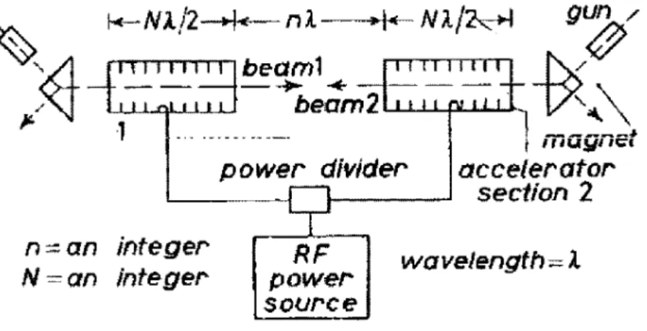
Originally the idea of ERL based facilities came from Maury Tigner [4]. He proposed an ERL based electron-electron collider (see Fig. 1.1). The scheme consists of two similar guns and two similar linear accelerators located coaxially. The beams start simultaneously from both sides, accelerate, collide in the middle, decelerate in the opposite linac and, finally they are dumped. In the same paper he proposed a scheme with one injector and one linac (Fig. 1.2).

But at that time the superconducting radio frequency (SRF) technology was not developed well enough and, therefore, it couldn’t be realized at that time. It required about 30-40 years of SRF development to achieve the feasible level for ERLs.

Figure 1.1: The first proposed scheme of ERL based e-e collider with two linacs.

Figure 1.2: The first proposed scheme of ERL based e-e collider with one linac.

(11)

Nowadays, operating ERLs already exist (Fig. 1.3 presents a map with the existing and proposed ERLs), like FEL in Novosibirsk [5], which was the first multi-turn ERL based FEL, but normal conductive, or FEL at the Japan Atomic Energy Research Institute (JAERI) [6], or the most powerful in the world (at the moment) FEL based on SRF ERL at Thomas Jefferson National Accelerator Facility [7]. There are also a few existing small scale facilities (with energies below 500 MeV), like ALICE at Daresbury [8], or S-DALINAC in Darmstadt [9].

Some of the test projects are under construction, like cERL at KEK [10], test ERL at Brookhaven National Laboratory [11], test facility at CERN [12], IHEP ERL in Beijing [13], Peking University ERL test facility [14], BERLinPro at Helmholtz-Zentrum Berlin (HZB) [15], etc. But all these projects and proposals are still relatively small with beam energies of hundreds MeVs. There is also a big number of proposed, let us call them, the large scale facilities with energy of some GeVs. There are proposed facilities with one turn, like ERL at Cornel University [16], or XFEL-O at KEK [17]. Also works are going on the multi-turn ERLs, like MARS in Novosibirsk [18] or FSF at HZB [19]. As one can see, there are a lot of projects of the ERL based light sources all over the world.

Figure 1.3: Existing and proposed facilities with an energy recovery linac for different

(12)

ERLs, as drivers, are attractive not only for synchrotron light sources. They can be used for several different applications. For example, ERL can be a very good driver for electron- hadron colliders. There are several proposed facilities like LHeC at CERN, or eRHIC at BNL [20, 21] or MEIC at JLab [22]. Another very attractive application of ERL is Coherent Electron Cooling [23]. It seems that ERL can be the only one suitable driver for it according to [24]. There are some proposals for internal target experiments, for example, MESA at Mainz [25, 26].

These projects might be realized with different acceleration and recovery schemes. In this work the different schemes for ERL based light source, as part of studies for BERLinPro and FSF projects, were compared.

1.1. BERLinPro

Helmholz-Zentrum Berlin has a project for the design and construction of the Berlin Energy Recovery Linac Project (BERLinPro) [15, 27, 28]. The main goal of the project is to demonstrate the potential of superconducting energy recovery linacs for high average current and low emittance operation. The schematic layout of the facility is shown in Fig. 1.4. The main parameters of BERLinPro are shown in Table 1.1.

Figure 1.4: The basic scheme of 100 MeV BERLinPro.

Originally the facility was planned to be built with a 100 MeV energy and 100 mA average current of an electron beam. But later, in order to guarantee the financial viability of the project, the beam energy was decreased to 50 MeV. What implied a shortening of the superconducting structures from 5 to 3 two-cell cavities in the booster and from 6 to 3 seven- cell cavities in the main linac. The new machine layout is shown in Fig. 1.5.

(13)

Table 1.1: The main parameters of BERLinPro

Parameter Value

Max. beam energy 100/50 MeV Average current up to 100 mA Max. repetition rate 1.3 GHz

Emittance < 1 mm mRad

Bunch length < 2 ps

Injection energy 7 MeV

A beam is generated in a 1.3 GHz SRF photo injector and, after it passes a three cavity booster section and a dog-leg merger, it comes to the main linac with energy of 6 MeV. Then it accelerates to 50 MeV, recirculates, decelerates back in the main linac and dumps in a 600- kW beam dump. In the recirculation arc there is also some available space for future experiments which can demonstrate the potential of ERL based machines for a huge number of user applications.

(14)

In Chapter 2 will be discussed both versions of BERLinPro and mostly the transverse Beam Breakup (BBU) instability in them. Since one of the main challenges of BERLinPro is to achieve a stable recirculation of the beam without a beam breakup [15]. BBU threshold currents for a different main linacs based on three different types of cavities: TESLA-type, CEBAF-type and cavities, which will be developed for BERLinPro, will be compared. A few methods of BBU instability suppression were applied for BERLinPro. These methods include: optimization of the Twiss parameters of a beam in the main linac or, betatron phase advances adjustment in the recirculation turn or, insertion of a so-called pseudo-reflector or solenoid, which interchange the transverse x and y coordinates of the betatron motion, etc.

The results are presented below.

Also, cavities which will be developed for BERLinPro can be used for the future large scale ERL based light source, which is currently under development at HZB.

1.2. FSF

Our group at Helmholtz Zentrum Berlin is designing a new future multi-turn energy recovery linac based light source with a two stage injection and with a maximum energy of electron beam about 6 GeV. This future facility is named Femto-Science Factory (FSF) [19].

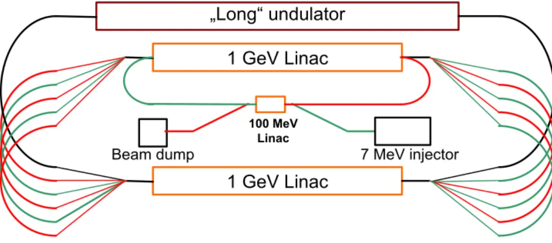
The problem of high brilliance SRF injectors is being intensively investigated as the injectors promise to deliver extremely low emittance bunches needed for the future linac- based light sources. An SRF injector with similar parameters to the BERLinPro injector under development at HZB [29, 30] is considered. A beam is created in SRF gun with photo cathode (see Fig. 1.6). Then it passes a 100 MeV linac, which is used as a first cascade in the acceleration. And then, the beam is accelerated to 6 GeV after passing 3 times through each of two 1 GeV main linacs. In the achromatic arcs between the acceleration stages it is assumed to have undulators with 1000 periods in each and in the long straight section a long undulator with 5000 periods is assumed. After the beam was used it is decelerated back and goes to a dump.

(15)

7 MeV injector Beam dump

1 GeV Linac

„Long“ undulator

100 MeV Linac

Figure 1.6: Principal layout of the multi-turn ERL with a cascade injection. The beam acceleration path is shown in green, deceleration path – in red.

The advantages and disadvantages of the two stage injection scheme with a split main linac will be discussed later in the next chapters. Now it should be noted, that the preinjection linac drastically improves the ratio between the initial and final energies on the first pass through the first 1 GeV linac. This improvement helps to make a reasonable focusing of the beam along the linac that improves the transverse beam break up instability of the facility.

The scheme with a split linac allows separation of the beams in the arcs for different passes (e.g. the beam on decelerating pass will have different energy compared to what it had on the accelerating pass). This means they are transported in different vacuum chambers. In this way all beams on all passes are separated and, therefore, users can see only one energy of a beam per arc in undulators (if installed in arcs with 1, 2…5 GeV energy).

(16)

The design was optimised to achieve a proposed wavelength of 1 Å in a diffraction limited regime.

To reach such a wavelength [31], undulators require a period d=2 cm and K=0.8:

Α

≈ +

= ) 1

1 2 2 (

2 2

K d

λ γ , (1.1)

for a 6 GeV beam.

Diffraction limited or spatially coherent regime reached when the transverse bunch size of a beam is smaller than σ (see Fig. 1.8) – the transverse “electron size” (size of single electron from the point of view of an observer of its light) in an undulator of length L=Npd and when the angular distribution of undulator radiation does not depends on the distribution of the particles in the beam, i.e. the angular spread is smaller than ψ – the radiation divergence angle for a single electron in an undulator. The ψ is given by [32]:

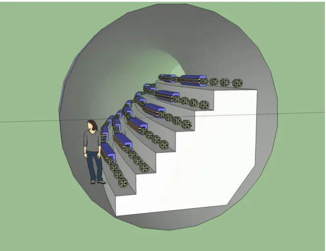
Figure 1.7: FSF arcs in a tunnel.

(17)

d N_p

ψ = λ . (1.2)

Ψ

L

σ

Figure 1.8: Source size of the undulator radiation.

The transverse electron size is given by:

d m N_p

π µ

σ λ 22

2 ≈

≈ , (1.3)

for an undulator with 1000 periods and d = 2 cm.

Therefore to work in diffraction limited regime a normalized emittance εn should be below:

μm 1 . 4 0

2 = ≈

≤ π

γ λ

ε_n γσψ _. _(1.4)

FSF is a large scale facility which should fulfil the requirements of its high number of users. The typical needs of synchrotron radiation users can be divided into four groups:

a) Maximal average brilliance in diffraction limited regime – requires a low emittance;

b) Maximal peak brilliance – requires low emittance and short bunch;

c) Minimal bunch length – requires short bunch;

d) And the last one is the experiments with high bunch degradation (e.g. ERL with FEL, e- p collider, internal target experiments, etc.) on which we don’t orient – requires large acceptance.

So, to achieve the record parameters which are above 3^rd generation light sources it is planned to have two operation modes. The 1^st mode will be optimized to provide a high brilliance beam. Another option is short bunch mode with a final beam minimal bunch length

(18)

Table 1.2: Main design parameters of FSF

Parameter High brilliance

mode Short bunch

mode

E, GeV 6 6

<I>, mA 20 5

Q, pC 15 4

τ, fs 200-1000 ~10

<B>, ph/s/mm²/mrad²/0.1% 8·10²² ~4·10²¹ Bpeak, ph/s/mm²/mrad²/0.1% 10²⁶ ~10²⁶

Accelerating gradient, MV/m 17

Energy gain per linac, GeV 1

f, GHz 1.3

So for the high brilliance mode it is proposed to have an average beam current I about 20 mA. The spectral brilliance of undulator radiation is given by [32]:

( ) ( )

ω σ ω σ σ σ π ω ω

d B N

y y x x

ph

′

= 4 2

 . (1.5)

So the maximum average brilliance can be written in a diffraction limited regime as:

( ) ( )

2 0 2

0 2 23

max 5 10 0.1

4

mrad mm

s

ph d

B N^ph

⋅

⋅ ⋅

>=

=<

>

<

ω ω λ

ω ^ ω , (1.6)

where the average photon flux is given by:

(K) e A d I N

N_ph _p ^av

ω πα ω

>=

<  , (1.7)

with A(K):

2 2

5 . 0 1

] ) [

( K

JJ K K

A = + (1.8)

and

2 2 2 )

1 2( 2 1 2 )

1 2(

1 4 2 4 2

]

[ 



 



 



 





− +



 





= +

+

− K

J K K

J K

JJ k k , (1.9)

(19)

where J is the Bessel function and α ~ 1/137 is a fine-structure constant. The estimation in (1.6) was done for K = 0.8, N = 1000 and I = 20 mA. Estimated value of an average brilliance is higher than for the 3^rd generation light sources (see Fig. 1.9).

Bunch compression is required to achieve high peak brilliance. The compression is subtle as not to spoil the emittance. The compression limit is set by the initial longitudinal emittance of the beam and by the effects of coherent and incoherent synchrotron radiation. With an average current of 20 mA, longitudinal size of 200 fs and peak current of 30 А one can likewise estimate the peak brilliance Bp.

2 0 2

0 2 26

1 . 10 0 4 7

mrad mm

s

ph N d

Bp = ph ≈ ⋅ ⋅ ⋅ ⋅

ω ω

 λ . (1.10)

A comparison between peak brilliance of 3^rd generation light sources, Free Electron Figure 1.9: Average brilliance of synchrotron light sources [33].

(20)

Let’s proceed with an optic in the arcs. Arcs are assumed to be similar and each arc consists of 6 30°-bending sections and 5 undulators with 1000 periods in between of them (Fig. 1.11). The bending section (Fig. 1.12) consists of 4 identical triple-bends with 4 quadrupoles on sides to match the following element (undulator or spreader). Each bending section in the 3-6 GeV arcs was optimized to suppress the emittance growth due to coherent and incoherent synchrotron radiations (CSR and ISR).

Figure 1.10: Peak brilliance of synchrotron light sources [33].

(21)

One of the main features of the arc design is that each triple bend has an anti-dipole magnet in the middle in order to achieve a zero R56 at reasonable strengths of quadrupoles.

The betatron phase advance Qx of each triple-bend section equals to 3/4 to cancel out the influence of CSR to the emittance [34]. The emittance growth due to incoherent synchrotron radiation can be written as [e.g. 35]:

5 5

3

2reCq I

x γ

ε =

∆ , (1.11)

where re is the classic radius of an electron, γ is the Lorentz factor of the beam, 1013

84 . 3 3

32

55 = ⋅ −

= mc

C_q 

m (1.12)

is a quantum constant and radiation integral I5 is given by:

∫

= H ds

I₅ ρ₃ ^, ^(1.13)

where ρ is the bending radius of dipoles and H is the Courant-Snyder parameter:

30⁰Achromatic ISR and CSR optimized sections

Undulators

Figure 1.11: Arc of FSF.

(22)

which depends on the dispersion η, its derivative and on the Twiss parameters of the beam.

Therefore, in order to suppress the emittance growth due to ISR, the Twiss parameters of the beam were optimized to minimize the radiation integral I5.

Another very important part of the accelerator layout is the spreader/recombiner sections.

The layout of the spreader after the second main 1 GeV linac is identical to the recombiner at the entrance to this linac and presented in the Fig. 1.13. The second pair of spreaders and recombiners for the first 1 GeV linac is identical, but without the 6 GeV beam line, which goes to the long undulator section. All spreader lines are isochronous.

One of the limiting factor for the spreader design is the contribution to the radiation integral I5, which characterizes the transversal emittance growth due to incoherent synchrotron radiation. Relatively high value of the horizontal β-function (50-100 m) from the linac section limits the bending angle of the separating dipoles (which represents η´).

Quadrupoles are necessary to minimize the contributions of other dipoles to I5, which in combination with isochronous and reasonable β-functions conditions requires a large number of them. Also a compact design is advantage for the installation footprint.

The difficulties (which grow with the number of the beam energies to be separated) originate from the conditions on the β-functions (low I5 contradicts with „natural“ β-functions out of the linacs) and dispersion (low I5 contradicts with the beam lines separation). To reduce the distances required for separation of the beams it was assumed to couple coordinates in the vertical plane. For this a magnet like a Lambertson separation septum [e.g. 36] for 4, 5, and 6 GeV beam lines (green in Fig. 1.13) is used. The coupling in the spreader makes the analysis and optimization of the spreader/recombiner section to be really complicated.

Figure 1.12: 30⁰ bending section of the FSF arc.

(23)

3m

26 m

(24)

(25)

2. Mode excitation by electron beam and BBU instability

In the superconducting cavities the electromagnetic fields might be expressed as sums of transverse magnetic (TM) and transverse electric (TE) modes. For TM modes there is a longitudinal electric field presented and a magnetic field could be everywhere perpendicularly to the longitudinal axis. For TE modes the situation is conversed with an existing longitudinal magnetic field and with electrical field transverse to it everywhere.

When a charge passes through a cavity it excites modes and induces fields which provide a retarding force. Some of the modes could be excited quite strong and lead to beam instabilities and finally to a beam loss.

At the beginning of this chapter formulas for the excitations of high order modes (HOMs) (as example for monopole and dipole modes) will be derived. When it is not specially linked then all the ideas in §2.1 and §2.2 are from [37]. One of these instabilities due to dipole modes – Beam Break Up instability will be discussed in the following paragraphs.

Different types of BBU instabilities will be discussed, such as single bunch BBU caused by short-range wakefields and two types of multi-bunch instabilities caused by long-range wakefields. As it will be shown later, one of the most problematic instabilities for the energy recovery linac based machines is a regenerative form of a transverse BBU. All types of BBU have a similar nature – they are caused by interaction of a beam with high order modes, but all of them are very different from each other. At the beginning single bunch BBU will be discussed, and then it will be continued with multi-bunch instabilities.

On one hand, some of the modes (eg. quadrupole modes) can lead to beam degradation that means the losses of luminosity for colliders or what is more important for us – the losses of brightness for synchrotron light sources. On the other hand, the excited modes give addition power dissipation in the cavity walls that increases the cryogenic losses.

At the end of this Chapter the modelling of the BBU instability for BERLinPro and the methods of BBU suppression will be discussed.

2.1. Monopole mode excitation

Modes of a cavity are independent from each other and form a complete orthogonal system and, therefore we can study the effects of the modes excitation individually for each mode. The final result will be given by a sum of all modes. Therefore let’s start with

(26)

First of all let’s determine the voltage induced by a point charge, moving on a cavity axis.

To do that the following facts will be used: first of all is that the energy in the system of a cavity and a charge is conserved, and the second that all fields excited by the charge may be added as superposition to any fields already existing in the cavity.

Let’s start with analysis of charges moving on axis. In this case only monopole TM modes can be excited because all other modes do not have any longitudinal electric field on the axis. Let the voltage, induced by the charge in one mode of the cavity be:

t i i q

q V e e ⁿ

V~ = ^α ⁻^ω , (2.1)

where Vq is the magnitude of the complex quantity 𝑉�_𝑞 and therefore is always positive, α is the phase between the charge and V�_q and ωn is the eigenfrequency of the mode.

One can continue with a postulate that the induced voltage also interacts with the charge itself. So, the effective voltage acting on the charge can be written as some fraction f of the total voltage:

q

eff fV

V~ = ~. (2.2)

To find the change in the voltage it is assumed that the cavity has no losses and it has been already excited to the voltage 𝑉�_𝑐:

t i i c

c Ve e ⁿ

V~ = ^ϕ ⁻^ω

, (2.3)

where the phase φ is an arbitrary angle at the time of passage and Vc is a positive real quantity.

Therefore, the initial stored energy in the cavity is given by:

0 2

Q VR

U a

n i c

ω

= , (2.4)

where Ra is the shunt impedance of the mode and Q0 is the unloaded quality factor. The final voltage, after the charge has passed the cavity, is given by the superposition:

0 2

Q R

e V e U V

n a q i c i

f ω

α ϕ +

= . (2.5)

The energy change in the cavity is:

(27)

0

) 2

cos(

2

Q R

V V

U V U U

n a

q q

i c f

c ω

α ϕ− +

=

−

=

∆ . (2.6)

The charge has also changed its energy:

) cos cos

( _c ϕ _q α

q qV fV

U = +

∆ . (2.7)

And, as it was said earlier, the energy of the whole system – charge-cavity is conserved and, therefore, one has:

0

=

∆ +

∆U_c U_q , (2.8)

that gives:

0

) 2

cos(

) 2 cos cos

(

Q R

V V

fV V V

q

n a

q q

c q

c ω

α α ϕ

ϕ+ = ⁻ ⁺

− , (2.9)

Now the superposition principle can be used. It requires Vq ~ q and in Eq. 2.9 one can equate the terms with the same powers of q:

0

) cos(

cos 2

Q R V qV V

n a q c c

ω

α

ϕ = ϕ⁻

− , (2.10)

0 2

cos

Q R qfV V

n a q q

ω α =

− , (2.11)

Since the phase φ is arbitrary, Eq. 2.10 can be true if α is 2π times an integer if q < 0, and π times an odd integer if q > 0. Therefore one find that:

t a i

q n qe ⁿ

Q

V ω R ₋^ω

= 2 0

~  (2.12)

and with Eqs. 2.2 and 2.12:

2

~ ~q eff

V =V . (2.13)

The quantity

ω R

(28)

is called a mode loss factor. It should be noted that the shunt impedance depends only on the geometry of the cavity and, therefore the loss factor as well. Using 2.4, one can find that:

U k_n V^c

4

= 2 . (2.15)

The Eq. 2.12 is given for point charge moving thought the lossless cavity. If it is required to include the losses, then the Eq. 2.12 still applies if the charge exits the cavity before the fields decayed substantially. The decay time is typically few microseconds or even longer (Q>>1) when the transit time of the charges is of the order of nanoseconds.

2.2. Dipole mode excitation

In the previous chapter the effect of monopole mode excitation in a cavity was studied. A monopole mode was excited by a charge moving on axis. It should be noted, that for all other modes the longitudinal electric field vanishes on axis. However, in a real accelerator bunches of charges perform some transverse oscillations about the design beam trajectory and therefore the other modes can be excited. In this chapter, using the same approach as in the previous chapter, excitation of dipole modes was studied.

Let’s start with a definition of a dipole loss factor kd, which is quite similar to the monopole mode loss factor (2.15). A force from a dipole mode on a charge increases linearly with a distance from the cavity axis therefore one need to choose a suitable reference distance. Let’s define Va as an accelerating voltage on the distance a – the beam pipe radius.

So, now a loss factor can be defined as:

U k_d V^a

4

= 2 . (2.16)

Now again, let a charge q to travel through a previously excited cavity with a stored energy of:

d

i ka

U V 4

2

= . (2.17)

And after the passage its energy might be written as:

d q i a i

f k

e V e U V

4

α 2 ϕ +

= . (2.18)

The phases φ and α have the same meanings as in the problem for monopole modes. Vq is the charge-induced voltage at the beam pipe radius.

(29)

The energy change of the charge moving at the distance ρ off the cavity axis is given by:

fV a V

q

U_q = ( _ccosϕ+ _qcosα)ρ

∆ . (2.19)

It should be noted that in Eq. 2.19 the field linearity in dependence on the offset from axis ρ was taken into account. As in the previous chapter, due to the energy conservation, now the energy change in the cavity and the energy gained by the charge can be equated. Again the superposition principle that (Vq ~ q) can be used, that gives:

k

a=2π , for integer k and q<0, (2.20) l

a=π , for odd integer l and q>0. (2.21) And one found:

t d i

q e ⁿ

q a k

V~ =2 ρ −^ω , (2.22)

where ρ ≤ a.

Due to the linear field variation with the distance from the axis the quantity Vρ/ρ is constant, where Vρ is the voltage at the distance ρ off axis. Therefore, the shunt impedance of a dipole mode can be defined as:

n c a

d a P

c V Q

R

2 2

2



 



=



 





ω , (2.23)

where Pc is the power, dissipated in the cavity walls. It should be noted that the defined shunt impedance is given in ohms (it is important for modeling). Now one can find the dipole loss factor:

0 2 2

4 Q R a c

k_d ωⁿ ωⁿ ^d



 



=  , (2.24)

where Q0 is the unloaded quality factor of the mode.

Dipole modes deflect a beam. And if they are strongly excited it could lead to a beam instability and finally to a beam loss. Especially this parasitic effect leads to so called beam break up instability in machines with energy recovery. This type of the instability will be discussed in the next sections.

(30)

2.3. Single bunch Beam Break Up

As it was discussed in the previous paragraphs the excited high order modes can be a reason for instabilities in Linear Accelerators. In this paragraph a single bunch BBU caused by short-range wakefields (for more details see e.g. [38, 39]) will be discussed. To illustrate the effect of this type of instability a two-particle model (shown in Fig. 2.1) for a bunch will be used. In this model it is assumed that the bunch consists of two ultrarelativistic macroparticles and each of them contains a half of the particles N/2 of the whole bunch. We assume the case of a smooth approximation that the head particle performs simple betatron oscillations with a frequency ωβ, which is independent of s, and, therefore:

) cos(

x~

= (s)

x_h _h kβs , (2.25)

where kβ=ωβ/c is the betatron wave number.

If the transverse wakefields are not induced by the head particle, then the tail particle would just follow the head.

When the wakefields are induced, the tail particle sees the deflecting wake field at the distance – σz behind and one can write the equation of motion for it, as:

) 2 (

) 2

( x s

L W x Nr

k

x_t _t ^e ^z _h

γ σ

β = ^⊥

′′+ , (2.26)

where re is the classical radius of an electron, σz is the beam size, γ is the relativistic factor corresponding to a beam energy and L is the length of the cavity period, 𝑊_⊥~2 𝑐𝑚⁻² is the transverse wake function taken at the distance 2σz behind the head particle. The solution of the Eq. 2.26 is given by:

Xt

Xh

Bunch of the particles

Figure 2.1: Two macroparticles model for single bunch BBU.

(31)











 +

= ^⊥ sin( )

4

) 2 ) (

cos(

x~

)

( _h s k s

L k W s Nr k s

x_t ^e ^z β

β

β γ

σ , (2.27)

where the first term describes just the betatron oscillations and the second term is the reaction to the wakefield left by the head particle.

Let’s continue with an introduction of a dimensionless, so called, instability growth parameter which is given by the ration of two amplitudes of the tail and the head:

2

4

) 2 1 (

~









 +

=

= ^e ^⊥ ^z _acc

h

t L

L k W Nr x

x

γ τ σ

β

, (2.28)

where Lacc is the total length of the linac. Usually 1 in the square root in Eq. 2.28 is neglected because it is assumed that there is instability with a high growth parameter >> 1.

Equation (2.28) was derived for the case without acceleration in the linac. As it was noted in [38], acceleration can be included by just replacing the factor Lacc/γ for its integral counterpart ∫₀^L^acc_γ(s)^ds =^L^acc_γ

f ln^γ_γ^f

i , where γi, (f) is the initial (final) relativistic factor.

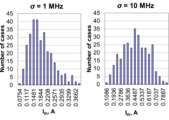
If we use now the parameters of the FSF beam presented in the Tab. 1.2, we get that the most unstable is the preinjection linac with a growth parameter τ ~1+2·10^{^-6}, that means that the tail is almost following to the head. Therefore, one can conclude that single bunch BBU is not a problem for the FSF facility. In the next paragraph another type of BBU instability – multi-bunch BBU in machines with energy recovery linac will be discussed.

(32)

2.4. Multi-bunch Beam Break Up instability

As it was shown in the previous chapter the single bunch BBU does not strongly influences the bunch of the FSF. In this chapter another type of instability will be discussed – multi-bunch BBU. It also has two forms – a cumulative and the most important for us a regenerative form of BBU instability.

The cumulative BBU occurs when there is no electromagnetic coupling between cavities but the dipole mode is excited in each cavity of the linac. The bunch is deflected in the first cavities by a dipole mode and excites the later cavities due to the off-axis position of the beam in the following cavities. The deflection grows with each cavity. Cumulative BBU is important for the facilities with a long linac.

Another form – so-called regenerative BBU occurs, when there is a strong electromagnetic coupling between the accelerating cavities. In this case the deflecting mode is like one mode in a multi-cell structure, when it moves synchronous with a beam, the beam get unstable. The excitation of the mode from the beam is carried electromagnetically from one cell to the next in the linac structure. The bunch is deflected in the first cavities and then it excites the later cavities or it excites the same cavity after recirculation so that the deviation is carried by the beam. This excitation grows with each bunch and, if the energy transfer to the cavity is greater than the ohmic losses of the cavity, then the instability develops.

This type of BBU instability can limit a beam current in the machines with energy recovery when the excitation is transferred by a bunch to the same mode on the recovery pass through the linac. Regenerative type of instability will be discussed in the next paragraphs.

2.4.1. Introduction to Regenerative Beam Break Up instability

One potential weakness of the ERLs is a regenerative form of transverse BBU instability, which may severely limit a beam current. The actuality of this problem was recognized in early experiments with the recirculating SRF accelerators at Stanford [40] and Illinois [41], where the average threshold current of this instability was about a few microamperes. In the works of Rand and Smith in [42] dipole high order modes were identified as a driver of this instability. In late 80’s the detailed theoretical model and simulation programs had been developed [43, 44]. Nowadays the interest to this problem was renewed. The requirements for more detailed theory and simulation programs [45-47] are given by the needs of high current (~100 mA) ERLs.

(33)

Let’s first briefly explain the fundamentals of the BBU instability. If an electron bunch passes through an accelerating cavity it interacts with dipole modes (e.g. TM110) in the cavity (Fig. 2.2). First, it exchanges energy with the mode; second, it is deflected by the electromagnetic field of the mode. After recirculation the deflected bunch interacts with the same mode in the cavity again and transfers the energy. If the net energy transfer from the beam to the mode is larger than the energy loss due to the mode damping then the beam becomes unstable.

Figure 2.2: Mechanism of BBU instability. On the left side schematically presented a layout of an ERL and trajectory kick due to a dipole mode. On the right side the fields in the transversal plane in this mode are presented.

Let’s start with a simple model of a single pass machine with one cavity and with one dipole mode in it. The length of the cavity is neglected and it is assumed that the mode gives a point like kick (so-called thin element approximation). Due to the fact, that the magnetic field of the mode is constant, one can assume that the bunch is one particle with the charge q.

So, at the first pass:



( )





−

′=

= ω sinϕ

0

1 1

ap x eV

x

a , (2.29)

where x1 is the coordinate (it is assumed that a beam moves on the axis on the 1-st pass and, therefore, there is no energy change) and 𝑥₁^′ is the kick angle, φ is the phase and p is the momentum of the bunch. After the pass through a recirculating ring with a transfer matrix M

= (m)ij, the bunch will come with an offset.

1 12

2 m x

x = ′. (2.30)

Ē

E H

(34)

1 12

2 cos( T )m x

a qV

U =− ^a + _r ′

∆ ϕ ω _. _(2.31)

Ohmic losses in the cavity were discussed earlier (Eq. 2.23) and can be expressed as:

Q Q a R c P V

d c a



 



 



 



=

2 2

2

ω ^. ^(2.32)

The threshold value is reached, when the ohmic losses and the average power deposited by individual bunches are equal:

2 > − =0

∆

< U f_b P_c . (2.33)

The averaging over the phase of the mode φ is done. This is possible due to assumption that the beams are moving with the frequency of the main acceleration mode, which is not a multiple to the frequency of the dipole mode therefore, the phase of the dipole mode at the beam passes is a random value normally distributed at [0; 2π]. The frequency fb at the threshold current is given by:

q I

f_b = _th/ . (2.34)

And now Eq. 2.33 leads to the final equation for the threshold current:

) sin(

2

12 2

r d

th

T Q Qm

e R I pc

ω ω _



 



− 

= . (2.35)

From Eq. 2.35 one can see that the threshold current is proportional to the beams energy.

It means that the most problematic cavities are where a beam has a lower energy. The threshold current is inversely proportional to:

- the impedance and the quality factor of the mode which should be minimized on a cavity design stage;

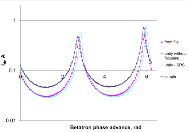
- the m12 matrix element, which for the case of a single mode and one cavity can be written as �𝛽₁𝛽2sin𝜇, where β1,2 – is a Twiss parameter of a beam on the 1^st and 2^nd passes correspondingly, should be minimized to achieve the highest threshold current.

The betatrone phase advance μ is additional optimization parameter.

It is required to know the phase of the mode φ, when the HOM frequency is equal to a harmonic number of the bunch repetition rate (M/N·fb, with integer M, N). In this resonant case the presented model does not provide the right solution. One has to calculate the phase

(35)

using some other method or some simulation program. It should be noted that the resonance cases should be avoided on the design stage by a proper choice of the beam frequency and of the cavity parameters. Also, Eq. 2.35 is true only for the case when the term m₁₂sin(ωT_r)<0_. This case perfectly agrees with simulation results as it was presented in [48]. Eq. 2.35 gives beams stability for the opposite case, when m₁₂sin(ωT_r)>0, but the simulation results show that the beam can be unstable with a high threshold current. This discrepancy caused by the assumption that the voltage induced by the beam on the second pass is very small compared to the HOM voltage, which fails at high bunch charges. In this case a more complicated theory is required. Such a theory was well described by G. Hoffstaetter and I. Bazarov in [45]. In the next paragraph the ideas are briefly summarized.

2.4.2. Regenerative BBU instability theory

In [45] the more general formulas for the BBU threshold current were derived. In principle authors used another approach to the same problem. In this part the main aspects of this paper are reviewed.

A simple model of one cavity and one dipole mode is assumed. If a mode is excited then a beam gets a transverse kick and after a recirculation it comes back to the cavity with an offset, and transfers the energy to the mode. If the energy of the mode increases, then the following bunches will experience the stronger kick that leads to the further energy grow of the mode and there is instability.

To describe this effect let’s start at a point of time t´, when the charge I(t´)dt´ with an offset x(t´) passes through the cavity on its deceleration loop and excites the HOM. The following particles on acceleration will see the transverse kick, which can be written as:

t d t I t x t t cW t e

px = − ′ ′ ′ ′

∆ ( ) ( ) ( ) ( ) , (2.36)

where W(τ) is the wake function which describes the transverse force at the time τ after the mode was excited.

An effective change of the transverse voltage of the HOM is given by:

) ( )

( p t

e t c

V = ∆ x

∆ . (2.37)

Now it can be assumed that all bunches are injected on the cavity axis and, therefore, they

(36)

time Tr. The transfer matrix element T12 = m12/p maps the transverse momentum px(t) to the offset:

) ( )

(t T T₁₂p t

x + _r = _x . (2.38)

Using (2.36) an integral equation for the effective voltage of the mode can be written as:

∫

∞

−

− ′

′

− ′

= ^t V t T_r dt

c T e t I t t W t

V( ) ( ) ( ) ₁₂ ( ) . (2.39)

To find the solution of this equation one can assume now that the current is a train of short bunches like the Diracs’s-delta functions with an intervals tb (see Fig. 2.3), so the current on the second deceleration pass is given by:

∑

^+∞

∞

−

=

−

=

m D r b

b t T mt

t I t

I( ) ₀ δ ( )_. _(2.40)

The time tb is proportional with some integer coefficient to an RF circulation time t0, which is inverse proportional to the main RF frequency ω0:

0

0 2

ω

= π

t . (2.41)

Now the recirculation time Tr can be written as:

b r

r n t

T =( −δ) . (2.42)

For an ERL δtb is given by:

) 0

2 (n 1 t t_b = +

δ _, _(2.43)

where n is integer.

Figure 2.3: Picture of time scales in the ERL.

(37)

Now, using (2.39) one can rewrite the effective voltage of the HOM at the time between some bunches t�[ntb+tr, (n+1)tb+tr] as:

∑

=−∞

−

= ⁿ

m r b b

b W t T mt V mt

c T e t I t

V( ) ₀ ₁₂ ( ) ( ). (2.44)

Let’s proceed at the time when the bunch passes through the cavity on the deceleration at the time t=ntb+tr:

∑

^∞

=

−

= +

12 0

0 ( ) (( ) )

) (

m b b

b r

b W mt V n m t

c T e t I T nt

V . (2.45)

As it was discussed §2.1 and §2.2, the voltage can be written as:

t

e i

V t

V( )= ₀ ⁻^ω . (2.46)

where a positive imaginary part of frequency ω indicates instability. Now (2.46) can be used in (2.45), that leads to the following equation:

∑

^∞

=

12 0 0

) 1 (

m

mt b i t

b ei ^r W mt e ^b

c T e I t

ω ω . (2.47)

The threshold current Ith is the smallest real value of the current I0 which corresponds to the real ω. In [45] authors used a Laplace transformation and wrote the dispersion relation as:

∑

^∞

=

+

=

12 0 0

) ] 1 ([

n

nt b i t

n

b ei ^r^b W n t e ^b

c T e I t

ω

ω δ _. _(2.48)

The sum in the dispersion relation (2.48) can be obtained in the far field approximation for the wakes. When the wake function can be written as:

τ ω ω

τ ^λ ^ω ^τ _λ

λ

λ sin

) 2

( ²e ⁽ ^/²^Q ⁾ c

Q

W R ⁻

 



= . (2.49)

The summation can be made as a geometric progression if Im(ω)>(-ωλ/2Qλ) and gives:

cos , cos

) ] 1 [ sin(

) sin(

4

) ] ([

) (

) 1 2 (

0

b b

t b b i

t t i

i n

nt b i

t t

t e

t e e

c Q R

e t n W w

b b

b

λ δ λ λ ω

δ ωδ ω λ λ

ω

ω ω

δ ω δ

ω ω

δ δ

−

 −



 



=

+

=

+

− −

∞

=

+ +

∑

(2.50)

where ω^± =ω ±i ω^λ and ω⁺ =ω+i ω^λ . Therefore, the equation for the current (2.48)

(38)

) ] 1 sin([

) sin(

)]

cos(

) [cos(

2 ²

12 0

b t b

i

b b

Q t t n i

t t

e

t t

e e I KT

b b b

r

λ ω λ

λ ω δ

ω

ω δ δ

ω

ω ω

λ λ

−

= − + −

− + , (2.51)

where ²₂

2c Q et R

K _b ^λ

λ

 ω



 



=  .

And now, for the case with energy recovery, when δ=1/2:

) 2 / sin(

) 2 / cos(

) cos(

1

12 0

b b

b t b

i

t t

t e t

I KT ^r

λ ω λ

ω ω

+

− + −

= . (2.52)

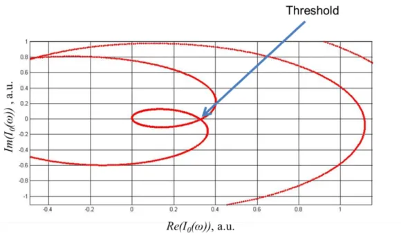
For a positive current I0 the values ω which corresponds to this value in the dispersion relation in principle will be a complex numbers. If the current is small then the imaginary parts of all of them are negative and the beam motion is stable. But when the current is increased then at some point one of them will become real. This point indicates the threshold current (see Fig. 2.4). So, the threshold current is the smallest real current I0 for which there is a real ω which satisfies the dispersion relation.

Figure 2.4: Dependence of I0(ω) in the complex plain in arbitrary units. The threshold point is indicated.

(39)

It should be noted that (2.52) can be simplified to (2.35) in the case of a single mode and one pass. Linearization and approximation that the HOM decay 1

2 t_b <<

Qλ

ωλ

is negligible in comparison to the bunch spacing tb is required^.

In the case of multiple recirculation turns and multiple HOMs in the cavities the solution can be found by the same approach as for a single mode and single recirculation case. One just has to introduce additional indexes for the numbering of the modes and of the recirculation turns. After that it should be carefully summarized and result will be found.

Here I would like to show the equation for a multi-pass ERL with one cavity and one mode in it, which was derived in [47]:

∑ ∑

⁻

= = +

≈ 2 1

1 2

0 N

m N

m

n m n

n eff m

b

QL I I

γ γ

β β

 , (2.53)

where I0- Alfven current, Q is the quality factor of HOM,  = λ/2π, λ is the wavelength corresponding to the resonant frequency of the TM110 mode, γm is the relativistic factor at the m-th pass through the cavity, βm – is the Twiss parameter, Leff – is the effective length of the cavity. This expression shows that it is preferable to have low β-functions at low energies. It also indicates the limitation for the number of passes.

For a modeling people have already developed computing codes, for example, TDBBU code developed at JLAB [49], MATBBU [50], the tracking code “bi” [51], GBBU code [52]

and etc. All of the codes have the same theoretical base. In the modeling GBBU code was used.

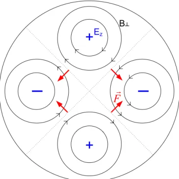
2.4.3. Regenerative BBU instability in a cavity with a quadrupole mode Instability of a beam in the field of a quadrupole mode of an accelerating cavity differs in the mechanism from the BBU in the field of a dipole mode.

Fig. 2.5 shows schematically the field distribution in a quadrupole mode. XY cross- section of a pillbox cavity, Ez and 𝐵_⊥ field lines, and force on the electron beam are shown.

The effect of the mode on the beam is, therefore, focusing in y and defocusing in x direction similar to a stationary quadrupole field but time dependent.