EVALUATION OF FUTURE
HYDROLOGICAL SCENARIOS USING STOCHASTIC
HIGH-RESOLUTION CLIMATE DATA
P. BURLANDO, N. PELEG, S. MORAGA-NAVARRETE, P. MOLNAR, S. FATICHI
IM AUFTRAG DES BUNDESAMTES FÜR UMWELT BAFU – NOVEMBER 2020 EIN FORSCHUNGSPROJEKT IM RAHMEN DES NCCS THEMENSCHWERPUNKTES
Impressum
Commissioned by: Federal Office for the Environment (FOEN), Hydrology Division, CH- 3003 Bern. The FOEN is an agency of the Federal Department of the Environment, Transport, Energy and Communications (DETEC)
Contractor: ETH Zürich, Versuchsanstalt für Wasserbau, Hydrologie und Glaziologie (VAW), HIA C58, Hönggerbergring 26, CH-8093 Zürich
Authors: Paolo Burlando(1), Nadav Peleg(1), Jorge Sebastián Moraga-Navarrete (1), Peter Molnar (1) and Simone Fatichi (1,2)
(1) Institute of Environmental Engineering, ETH Zurich
(2) Department of Civil and Environmental Engineering, National University of Singapore
FOEN support: Fabia Huesler, Petra Schmocker-Fackel
Note: This study/report was prepared under contract to the Federal Office for the Environment (FOEN). The contractor bears sole responsibility for the content.
Citation: Burlando, P., Peleg, N., Moraga-Navarrete, J.S., Molnar, P., and Fatichi, S. 2020.
Evaluation of future hydrological scenarios using stochastic high-resolution climate data. Com- missioned by the Federal Office for the Environment (FOEN), Bern, Switzerland. 50 pp, DOI:10.3929/ethz-b-000462637
DOI: 10.3929/ethz-b-000462637
Authors: P. Burlando, N. Peleg, S. Moraga-Navarrete, P.Molnar and S. Fatichi Chair of Hydrology and Water Resources Management, ETH Zurich
https://hyd.ifu.ethz.ch
Table of Contents
1 INTRODUCTION ... 1
2 METHODS ... 2
2.1 THE AWE-GEN-2D MODEL ... 2
2.2 TOPKAPI-ETHHYDROLOGICAL MODEL ... 3
2.3 FROM CLIMATE TO HYDROLOGICAL PREDICTIONS ... 3
3 STUDY CATCHMENTS ... 4
4 DATA ... 6
5 RESULTS ... 7
5.1 VALIDATION OF AWE-GEN-2D ... 7
5.2 VALIDATION OF TOPKAPI-ETH ... 12
5.3 CHANGES IN CLIMATE ... 15
5.3.1 Domain scale ... 15
5.3.2 The 2-km scale ... 19
5.4 CHANGES IN HYDROLOGY ... 21
5.4.1 Changes of the mean streamflow regime at the catchment outlets (Kl. Emme and Thur) ... 21
5.5 CHANGES TO THE MEAN INFLOWS INTO THE RESERVOIRS IN THE MAGGIA BASIN ... 31
5.5.1 Changes to extreme flows in the Kl. Emme and Thur ... 33
6 CONCLUSIONS ... 37
7 REFERENCES ... 38
List of Tables
Table 1 – List of ground stations from MeteoSwiss. ... 6 Table 2 – List of climate models from the CH2018 archive that were used in this project. ... 7 Table 3 – List of streamflow recording stations that were used in this project. ... 7
List of Figures
Figure 1 – A schematic representation of the methodological modelling framework. Points 1 to 7 are detailed described in Section 2.3. ... 2 Figure 2 – Location map of the catchments. Coordinates are in Swiss projection (CH-1903) in m. ... 5 Figure 3 – Mean near-surface air temperature for the period 1982-2015 as obtained from the TabsY
product (observed) in comparison with the mean ensemble generated by AWE-GEN-2d (simulated).
... 9 Figure 4 – Mean precipitation for the period 1982-2015 as obtained from the RhiresD product (observed) in comparison with the mean ensemble generated by AWE-GEN-2d (simulated). ... 10 Figure 5 – Observed mean diurnal cycle of temperature (blue) and simulated (red) computed from the
generated climate ensemble. Location: Luzern – Kl. Emme, Aadorf – Thur, and Locarno – Maggia.
... 10 Figure 6 – A comparison between observed and simulated temperatures for each month. The blue and red solid lines represent the observed and simulated median values (respectively) and the bounded areas represent the observed (blue area) and simulated (dashed lines) 5–95th percentile range
(respectively). The observed period covers 34 years of data (1982–2015), while simulations
represent the mean of 30 realizations of 30 years each. ... 11 Figure 7 – A comparison between observed and simulated precipitation for each month. The blue and red solid lines represent the observed and simulated median values (respectively) and the bounded areas represent the observed (blue area) and simulated (dashed lines) 5–95th percentile range
(respectively). The observed period covers 34 years of data (1982–2015), while simulations
represent the mean of 30 realizations of 30 years each. ... 11 Figure 8 – Validation of annual maximum precipitation intensity at the hourly scale for different return
periods in the Kl. Emme (top row) and Thur (bottom row) weather stations. The solid lines represent the observed (blue) and simulated (red) precipitation intensity computed by fitting GEV distribution to the data. The observed period covers 34 years of data (1982–2015), while simulations represent the mean of 30 realizations of 30 years each. ... 12 Figure 9 – A comparison between observed and simulated inflow for each month (2006-2015, excluding
2010) in Sambuco reservoir. The blue and red lines represent the observed and simulated mean values (respectively). ... 13 Figure 10 – A comparison between observed (blue) and Topkapi-ETH simulated (red) streamflow (outlet
of Kl. Emme catchment). NSE refers to the Nash–Sutcliffe efficiency that was computed at the hourly scale for the period 2000-2009. ... 13 Figure 11 – A comparison between observed and simulated streamflow for each month (2000-2009). The blue and red solid lines represent the observed and simulated median values (respectively) and the bounded areas represent the observed (blue area) and simulated (dashed lines) 5–95th percentile range (respectively). ... 14 Figure 12 – Comparison between observed and simulated peak-over-threshold at the hourly scale for
different return periods in the Kl. Emme (left) Thur (right) catchments. The solid lines represent the observed (blue) and simulated (red) streamflow computed by fitting a Generalized Pareto
distribution to the recorded data for the 2000–2009 period. The plotting positions were calculated using Gringorten’s equation and the return periods are calculated via the reduced variate method. . 14 Figure 13 – Differences in mean annual temperature between the present period (1976-2005) and future
periods for the Kl. Emme, Thur and Maggia catchments. Numbers 1 to 9 refer to the different climate models (see Table 1) and MMM refers to the multi-model mean. Box plots for the present
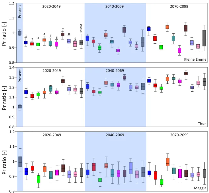
plots represent the median of the mean annual temperature of the ensemble, while the boxes and whisker lines represent the 25-75th and 5-95th percentile range of the data. The simulated ensemble for each climate trajectory is composed of 30 realizations of 30 years each, bootstrapped from an archive of 100 years. ... 16 Figure 14 – Similar plot as Fig. 13, but for the ratios of mean annual precipitation. ... 17 Figure 15 – The ratio between annual maximum precipitation for a given return period of present climate (1976-2005) and end of the century climate (2070-2099) at the hourly scale. Numbers 1 to 9 refer to the different climate models (see Table 1) and M refers to the multi-model mean. Box plots for the present and 1 to 9 represent the stochastic uncertainty for each climate trajectory, and M represents the combination of stochastic and climate model uncertainty. Central lines in the box plots represent the median of mean annual maximum precipitation intensity computed from the simulated ensemble using GEV distribution, while the boxes represent the 5-95th percentile range of the data. The simulated ensemble for each climate trajectory is composed of 30 realizations of 30 years each, bootstrapped from an archive of 100 years. ... 18 Figure 16 – Similar plot as Fig. 15, but on a daily scale. ... 19 Figure 17 – Projected multi-model mean anomalies in climate variables relative to the present climate
(1976–2005) in the Kl. Emme (a–d), Thur (e–h) and Maggia (i-l). Panels (a, e), (c, g) and (i, k) show the monthly precipitation and temperature anomalies for each future period, respectively, whereas panels (b, f), (d, h) and (j, l) show the spatial distribution of the annual anomaly by the end of the century (2080–2089). ... 20 Figure 18 – Differences in the temperature of the hottest day in the year (annual maximum of daily Tmax,
TXx) and ration change of mean daily rainfall (MEA) between the present climate (1976-2005) and end of the century scenarios (2070-2099, multi-model mean). ... 21 Figure 19 – Differences in mean annual streamflow between the present and future periods for the Kl.
Emme and Thur catchments. Numbers 1 to 9 refer to the different climate models and M refer to the multi-model mean. Box plots for the present and 1 to 9 represent the stochastic uncertainty for each climate trajectory, and M represents the combination of stochastic and climate model uncertainty.
Central lines in the box plots represent the median of mean annual streamflow of the ensemble, while the boxes and whisker lines represent the 25-75th and 5-95th percentile range of the data. The simulated ensemble for each climate trajectory is composed of 30 realizations of 30 years each, bootstrapped from an archive of 100 years. ... 22 Figure 20 – The ratio between monthly streamflow of present (1976-2005, grey), early-mid-century
(2020-2049, blue), mid-century (2040-2079, red) and end of the century (2070-2099, yellow) periods. Box plots for the present period represent the stochastic uncertainty for the future periods represent the combination of stochastic and climate model uncertainty. Central lines in the box plots represent the median of mean monthly streamflow computed from the simulated ensemble, while the boxes represent the 5-95th percentile range of the data. The simulated ensemble for each climate trajectory is composed of 30 realizations of 30 years each, bootstrapped from an archive of 100 years. ... 23 Figure 21 – Change in mean effective saturation (a, b), snow water equivalent (c, d) and annual
evapotranspiration (e, f) for the Kl. Emme and Thur catchments. All values correspond to the averages of the multi-model-mean (MMM) at the end of the century (2080–2089) minus the present climate condition. ... 24 Figure 22 – Differences in snow water equivalent (SWE) between the present and future periods for the
Kl. Emme and Thur catchments. Numbers 1 to 9 refer to the different climate models and M refer to the multi-model mean. Box plots for the present and 1 to 9 represent the stochastic uncertainty for each climate trajectory, and M represents the combination of stochastic and climate model
uncertainty. Central lines in the box plots represent the median of mean SWE of the ensemble, while
the boxes and whisker lines represent the 25-75th and 5-95th percentile range of the data. The simulated ensemble for each climate trajectory is composed of 30 realizations of 30 years each, bootstrapped from an archive of 100 years. ... 25 Figure 23 – Average snow height in the Kl. Emme catchment for the present period (left) and end of the
century (right, multi-model-mean). ... 25 Figure 24 – Monthly streamflow (thick black line) and its hydrological components at the outlet of the Kl.
Emme (a, c) and Thur (b, d) river catchments for the present climate (a, b) and the changes projected towards the end of the century (2080–2089, c, d). The bars corresponding to evapotranspiration (blue) and an increase in soil water volume (pink) are depicted as negative contributions to the water balance. ... 26 Figure 25 – Spatial distribution of 96 sub-catchments in the Kl. Emme river network (a) and 140 of the
Thur river network (b). River reaches are drawn according to their Strahler order and markers are coloured based on their average specific annual discharge in the present climate. ... 27 Figure 26 – Impacts on streamflow in 97 Kl. Emme river sub-catchments (a, c, e) and 140 Thur river sub-
catchments (b, d, f). The change rates between the present climate and the end of the century are computed for each river section are shown for the maximum hourly flow (a, b), mean flow (c, d) and 7-day minimum flow (e, f). The markers in all plots are colored according to the mean specific streamflow in the present climate, and the river section corresponding to the outlet of the entire catchment is highlighted with a black border. ... 28 Figure 27 – Most important (a–d) and second most important (e–h) driver of seasonal flow in the Kl.
Emme river network under present (circles) and future (triangles) climate conditions. ... 29 Figure 28 – Similar to Fig. 27, but for the Thur river basin. ... 30 Figure 29 – Schematic representation of the hydro-power reservoirs in the Maggia river basin. Image is
from OFIMA website1. ... 31 Figure 30 – Differences in mean annual inflow to the reservoirs between the present and future periods.
Numbers 1 to 9 refer to the different climate models and M refer to the multi-model mean. Box plots for the present and 1 to 9 represent the stochastic uncertainty for each climate trajectory, and M represents the combination of stochastic and climate model uncertainty. Central lines in the box plots represent the median of mean annual streamflow of the ensemble, while the boxes and whisker lines represent the 25-75th and 5-95th percentile range of the data. The simulated ensemble for each climate trajectory is composed of 30 realizations of 30 years each, bootstrapped from an archive of 100 years. ... 32 Figure 31 – The ratio between monthly inflow into the reservoirs of the present (1976-2005, grey), early-
mid century (2020-2049, blue), mid-century (2040-2079, red) and end of the century (2070-2099, yellow) periods. Box plots for the present period represent the stochastic uncertainty for the future periods represent the combination of stochastic and climate model uncertainty. Central lines in the box plots represent the median of mean monthly streamflow computed from the simulated
ensemble, while the boxes represent the 5-95th percentile range of the data. The simulated ensemble for each climate trajectory is composed of 30 realizations of 30 years each, bootstrapped from an archive of 100 years. ... 33 Figure 32 – The ratio between annual maximum streamflow for a given return period of present climate
(1976-2005) and end of the century climate (2070-2099) at the hourly scale. Numbers 1 to 9 refer to the different climate models and M refer to the multi-model mean. Box plots for the present and 1 to 9 represent the stochastic uncertainty for each climate trajectory, and M represents the combination of stochastic and climate model uncertainty. Central lines in the box plots represent the median of
climate trajectory is composed of 30 realizations of 30 years each, bootstrapped from an archive of 100 years. ... 35 Figure 33 – Similar plot as Fig. 22, but on a daily scale. ... 35 Figure 34 – Monthly frequency of the hourly (a, c) and daily (b, d) maximum yearly outlet streamflow
occurring in each month in the Kl. Emme (a-b) and Thur (c-d) rivers. ... 36 Figure 35 – Similar plot as Fig. 22, but for NM7Q. Note that for the GEV calculation the minimum
annual streamflow was multiple by -1. ... 36
Summary
The present report illustrates the outcomes of a project aimed to analyse the detailed and spatio- temporal highly-resolved impact of climate change on the hydrological response of three catch- ments in Switzerland, Thur, Kl. Emme and Maggia.
This project is part of the NCCS efforts to explore climate change impacts on hydrology in Swit- zerland and is unique in three aspects. First, it allows for the first time the investigation of cli- mate impacts on the hydrology at sub-daily (hourly) scales; second, it enables exploring the ef- fects of the natural (stochastic) climate variability on the hydrological components, thus allowing better estimation of the expected uncertainty in future hydrological predictions; and third, it al- lows the detailed exploration of the changes affecting the hydrological components within the catchments also exploring them at the grid cell or sub-catchment scales. To that end, high tem- poral and spatial resolution gridded climate variables, characterised by hourly and hundreds of meters scales, i.e. much finer resolution than that of the MeteoSwiss CH2018 official scenarios, were stochastically simulated using the advanced state-of-the-art AWE-GEN-2d weather genera- tor model to form ensembles representing the future climate for the highest greenhouse-gasses emission scenario (RCP8.5). The fully distributed physically-based hydrological model Topkapi- ETH, capable of simulating streamflow and the other land components of hydrological processes over complex terrain, was used to estimate the changes affecting the key hydrological compo- nents in space and time.
The projected changes in temperatures are characterized by high uncertainty. The temperatures in the Kl. Emme and Thur catchments are projected to increase in a range of 0.4-2 °C, 1.4-3 °C and 2.7-5.3 °C when comparing the periods of 2020-2049, 2040-2069 and 2070-2099 (respec- tively) to the present climate (1976-2005). A higher increase in temperatures is projected in the Maggia catchment, in the order of 3.4-6 °C for the end of the century. Model results suggest a spatially uniform increase in temperature over the catchments.
The magnitude and spatial patterns of change in precipitation differ between catchments. While in the Kl. Emme and Maggia catchments a general decrease in precipitation is predicted, an in- crease in precipitation is projected in the Thur catchment. The decrease in precipitation in the Kl.
Emme and Maggia catchments is associated with high uncertainties: -15% to +3%, -18% to +6%
and -17% to +8% for the periods 2020-2049, 2040-2069 and 2070-2099 (respectively) in com- parison to the period of 1976-2005. The change in precipitation considerably overlapped with the present natural precipitation variability that is in the order of ±5%. The increase in precipitation in the Thur catchment exceeds the present natural precipitation variability. The change is pro- jected in the range of +6% to +33%, +9% to +34% and +14% to +40% for the same periods as mentioned above. In the Kl. Emme and Thur catchments, precipitation tends to decrease in fu- ture climate over the mountainous regions and increase in the low elevation areas, while in the Maggia catchment precipitation is generally decreasing, with a higher magnitude of decrease over the mountainous areas in comparison to the lower areas. Extreme rainfall intensities at the hourly scale are characterized with high natural variability, in the order of ±10% for the 2-year return period and ±30% for the 30-year return period in all catchments. The uncertainty in the
Climate change is predicted to affect the hydrological components in the catchments. The nota- ble changes are a meaningful decrease in snowmelt during spring – snowmelt contribution to the streamflow is expected to decrease by 50% (for both catchments) at the end of the century – and an increase in summer evapotranspiration in the order of 10%. Model results indicate a decrease in mean annual streamflow for the Kl. Emme and Thur catchments in future climates – up to - 23% in comparison to the present – with the most meaningful change already occurring in the period 2020-2049. However, the uncertainty in future streamflow predictions is high, with some climate models forcing an increase in streamflow up to 5% and 12% for the Kl. Emme and Thur catchments, respectively. For both catchments, winter flows are predicted to increase and sum- mer flows are predicted to decrease, with magnitudes and uncertainties increasing toward the end of the century. In the Maggia, spatially different responses to climate change were detected – e.g.
a decrease in inflows was found to the large reservoirs (e.g. Sambuco), while small reservoirs could experience an increase in inflows.
In terms of changes to streamflow extremes, no changes in the statistics of maximum annual streamflow at the hourly scale were identified for the high-frequency (2-year return period) flows in the Kl. Emme and Thur catchments. For lower frequency hourly annual maximum flows (i.e. 30-year return period) it is impossible to identify a clear change signal as the uncertainty in the change is very high (-40% to +60%) and largely matches the stochastic variability of present- day climate. Most models, however, agree on a reduction in low-flows statistics in the Kl. Emme and Thur catchments, where a median reduction of 25% is foreseen for the 7-day low-flows sta- tistics at the end of the century. Moreover, all downscaled climate trajectories agree that hourly streamflow extremes will become less frequent during summer – remaining this season the main period of flood occurrences – and more frequent during winter.
Zusammenfassung
Der vorliegende Bericht veranschaulicht die Ergebnisse eines Projekts, das darauf abzielte, die detaillierten und räumlich-zeitlich hoch aufgelösten Auswirkungen des Klimawandels auf die hydrologische Reaktion von drei Einzugsgebieten in der Schweiz, Thur, Kl. Emme und Maggia zu analysieren.
Dieses Projekt ist Teil der NCCS-Bemühungen zur Erforschung der Auswirkungen des Klima- wandels auf die Gewässersysteme in der Schweiz und ist in dreierlei Hinsicht einzigartig. Ers- tens ermöglicht es zum ersten Mal die Untersuchung der Klimaauswirkungen auf die Gewässer- systeme auf untertägiger (stündlicher) Skala; zweitens ermöglicht es die Erforschung der Aus- wirkungen der natürlichen (stochastischen) Klimavariabilität auf die hydrologischen Komponen- ten, was eine bessere Abschätzung der erwarteten Unsicherheit in zukünftigen hydrologischen Vorhersagen ermöglicht; und drittens ermöglicht es die detaillierte Erforschung der Veränderun- gen, die die hydrologischen Komponenten innerhalb der Einzugsgebiete betreffen, auch auf der Skala der Rasterzellen oder Untereinzugsgebiete. Zu diesem Zweck wurden zeitlich und räum- lich hoch aufgelöste gerasterte Klimavariablen, die sich durch stündliche und Hunderte von Me- tern Skalen auszeichnen, d.h. eine viel feinere Auflösung als die der offiziellen CH2018-Szena- rien von MeteoSwiss, stochastisch mit dem hochmodernen AWE-GEN-2d Wettergeneratormo- dell simuliert, um Ensembles zu bilden, die das zukünftige Klima für das höchste Treibhausgas- Emissionsszenario (RCP8.5) abbilden. Das vollständig ausgebaute, physikalisch basierte hydro- logische Modell Topkapi-ETH, das in der Lage ist, den Flusslauf und die anderen Landkompo- nenten der hydrologischen Prozesse in komplexem Gelände zu simulieren, wurde verwendet, um die Änderungen abzuschätzen, die die wichtigsten hydrologischen Komponenten in Raum und Zeit betreffen.
Die projizierten Änderungen der Temperaturen sind durch hohe Unsicherheiten gekennzeichnet.
Die Temperaturen in den Einzugsgebieten Kl. Emme und Thur werden in einem Bereich von 0,4-2 °C, 1,4-3 °C und 2,7-5,3 °C ansteigen, wenn man die Zeiträume 2020-2049, 2040-2069 und 2070-2099 (jeweils) mit dem heutigen Klima (1976-2005) vergleicht. Im Maggia-Einzugs- gebiet wird ein höherer Temperaturanstieg prognostiziert, in der Grössenordnung von 3,4-6 °C für das Ende des Jahrhunderts. Die Modellergebnisse deuten auf einen räumlich gleichmässigen Temperaturanstieg in den Einzugsgebieten hin.
Das Ausmass und die räumlichen Muster der Niederschlagsänderung unterscheiden sich zwi- schen den Einzugsgebieten. In den Einzugsgebieten Kl. Emme und Maggia wird eine generelle Abnahme des Niederschlags vorhergesagt, wohingegen im Einzugsgebiet Thur eine Zunahme des Niederschlags erwartet wird. Die Abnahme des Niederschlags in den Einzugsgebieten Kl.
Emme und Maggia ist mit hohen Unsicherheiten verbunden: -15% bis +3%, -18% bis +6% und - 17% bis +8% für die Perioden 2020-2049, 2040-2069 und 2070-2099 (jeweils) im Vergleich zur Periode 1976-2005. Die Änderung des Niederschlags überschneidet sich erheblich mit der ge- genwärtigen natürlichen Niederschlagsvariabilität, die in der Grössenordnung von ±5% liegt. Die Niederschlagszunahme im Einzugsgebiet Thur übersteigt die derzeitige natürliche Nieder-
schlagsvariabilität. Die Änderung wird im Bereich von +6% bis +33%, +9% bis +34% und
Gebirgsregionen tendenziell ab und in den tiefer gelegenen Gebieten zu, wohingegen im Ein- zugsgebiet der Maggia der Niederschlag generell abnimmt, wobei die Abnahme über den Ge- birgsregionen im Vergleich zu den tiefer gelegenen Gebieten stärker ausfällt. Extreme Nieder- schlagsintensitäten auf der stündlichen Skala sind durch eine hohe natürliche Variabilität ge- kennzeichnet, in der Grössenordnung von ±10% für die 2-jährige Wiederkehrperiode und ±30%
für die 30-jährige Wiederkehrperiode in allen Einzugsgebieten. Die Unsicherheit in der Verände- rung der extremen Niederschlagsintensität liegt in der gleichen Grössenordnung wie die natürli- che Variabilität und überschneidet sich weitgehend mit ihr, was die Erkennung eindeutiger Trends erschwert.
Es wird vorhergesagt, dass der Klimawandel die hydrologischen Komponenten in den Einzugs- gebieten beeinflussen wird. Die bemerkenswerten Änderungen sind ein deutlicher Rückgang der Schneeschmelze im Frühjahr – der Beitrag der Schneeschmelze zum Abfluss des Flusses wird bis zum Ende des Jahrhunderts voraussichtlich um 50% (für beide Einzugsgebiete) abnehmen – und ein Anstieg der Verdunstung im Sommer in der Grössenordnung von 10%. Die Modeller- gebnisse zeigen eine Abnahme des mittleren jährlichen Abflusses für die Einzugsgebiete Kl.
Emme und Thur in zukünftigen Klimaten – bis zu -23% im Vergleich zu heute – wobei die be- deutendste Änderung bereits in der Periode 2020-2049 auftritt. Allerdings ist die Unsicherheit in den zukünftigen Abflussvorhersagen hoch, wobei einige Klimamodelle einen Anstieg des Ab- flusses um bis zu 5% und 12% jeweils für die Einzugsgebiete Kl. Emme und Thur vorhersagen.
Für beide Einzugsgebiete wird eine Zunahme der Winterabflüsse und eine Abnahme der Som- merabflüsse vorhergesagt, wobei die Grössenordnungen und Unsicherheiten gegen Ende des Jahrhunderts zunehmen. In Maggia wurden räumlich unterschiedliche Reaktionen auf den Kli- mawandel festgestellt – z.B. wurde eine Abnahme der Zuflüsse zu den grossen Stauseen (z.B.
Sambuco) festgestellt, wohingegen kleine Stauseen eine Zunahme der Zuflüsse erfahren konn- ten.
In Bezug auf Änderungen der Abflussextreme wurden keine Änderungen in der Statistik der ma- ximalen jährlichen Abflüsse auf der Stundenskala für die hochfrequenten (2-jährige Wiederkehr- periode) Abflüsse in den Einzugsgebieten Kl. Emme und Thur festgestellt. Für die niederfre- quenten stündlichen jährlichen Maximalabflüsse (d.h. 30-jährige Wiederkehrperiode) ist es un- möglich, ein klares Änderungssignal zu identifizieren, da die Unsicherheit der Änderung sehr hoch ist (-40% bis +60%) und weitgehend mit der stochastischen Variabilität des heutigen Kli- mas übereinstimmt. Die meisten Modelle stimmen jedoch überein, dass die Niedrigwasserzahlen in den Einzugsgebieten von Kl. Emme und Thur abnehmen werden, wobei für die 7-tägigen Niedrigwasserzahlen am Ende des Jahrhunderts eine mittlere Abnahme von 25 % vorhergesagt wird. Darüber hinaus stimmen alle herunterskalierten Klimaprognosen darin überein, dass stünd- liche Abflussextreme im Sommer seltener werden – diese Jahreszeit bleibt die Hauptperiode für Hochwasserereignisse – und im Winter häufiger auftreten werden.
Résumé
Le présent rapport illustre les résultats d'un projet visant à analyser l'impact détaillé et à haute ré- solution spatio-temporelle du changement climatique sur la réponse hydrologique de trois bas- sins versants en Suisse, de la Thur, la Petite Emme et la Maggia.
Ce projet fait partie des efforts du NCCS pour étudier les impacts du changement climatique sur l'hydrologie en Suisse et est unique en trois aspects. Premièrement, il permet pour la première fois l'étude d'impacts climatiques sur l'hydrologie à des échelles sous-quotidiennes (horaires) ; deuxièmement, il permet d'étudier les effets de la variabilité climatique (stochastique) naturelle sur les composants hydrologiques, permettant ainsi une meilleure estimation de l'incertitude at- tendue dans de futures prévisions hydrologiques ; et troisièmement, il permet l'exploration détail- lée des changements affectant les composants hydrologiques dans les bassins versants, les explo- rant aussi à l'échelle de cellules de grille ou de sous-bassins versants. À cette fin, des variables climatiques grillées à haute résolution temporelle et spatiale, caractérisées par des échelles ho- raires et de centaines de mètres, c'est-à-dire une résolution bien plus fine que celle des scenarios officiels CH2018 de MeteoSwiss, ont été simulées de manière stochastique en utilisant le modèle de pointe de génération de données météorologiques AWE-GEN-2d pour former des ensembles représentant le climat futur pour le scenario des émissions de gaz à effet de serre les plus élevées (RCP8.5). Le modèle hydrologique Topkapi-ETH entièrement distribué basé sur la physique, ca- pable de simuler l'écoulement fluvial et les autres composants terrestres de processus hydrolo- giques sur des terrains complexes, a été utilisé pour estimer les changements affectant les com- posants hydrologiques clé dans l'espace et le temps.
Les changements projetés de température sont caractérisés par une incertitude élevée. Les tempé- ratures dans les bassins versants de la Petite Emme et de la Thur sont prévues d'augmenter dans une plage de 0,4 à 2 °C, 1,4 à 3 °C et 2,7 à 5,3 °C lors de la comparaison des périodes 2020- 2049, 2040-2069 et 2070-2099 (respectivement) au climat actuel (1976-2005). Une augmenta- tion plus importante des températures est prévue dans le bassin versant de la Maggia, de l'ordre de 3,4 à 6 °C pour la fin du siècle. Les résultats de modèles suggèrent une augmentation spatiale- ment uniforme des températures le long des bassins versants.
L'ampleur et les modèles spatiaux des changements dans les précipitations varient entre les bas- sins versants. Alors qu'une réduction générale des précipitations est prédite dans les bassins ver- sants de la Petite Emme et de la Maggia, une augmentation des précipitations est prévue dans le bassin versant de la Thur. La réduction des précipitations dans les bassins versants de la Petite Emme et de la Maggia est associée à des incertitudes élevées: -15% à +3%, -18% à +6% et -17%
à +8% pour les périodes de 2020-2049, 2040-2069 et 2070-2099 (respectivement), par rapport à la période de 1976-2005. Le changement dans les précipitations s'est recoupé fortement avec la variabilité naturelle actuelle des précipitations, qui est de l'ordre de ±5%. L'augmentation des précipitations dans le bassin versant de la Thur dépasse la variabilité naturelle actuelle des préci- pitations. Le changement est prévu être dans la plage de +6% à +33%, +9% à +34% et +14% à +40% pour les mêmes périodes que celles mentionnées ci-dessus. Dans les bassins versants de la Petite Emme et de la Thur, les précipitations tendent à diminuer, dans le climat futur, le long des
ordre de grandeur supérieur le long des régions montagneuses par rapport aux zones plus basses.
Les intensités des précipitations extrêmes à l'échelle horaire sont caractérisées par une variabilité naturelle élevée, de l'ordre de ±10% pour la période de retour de 2 ans et de ±30% pour la pé- riode de retour de 30 ans dans tous les bassins versants. L'incertitude dans le changement de l'intensité des précipitations extrême est du même ordre de grandeur que la variabilité naturelle et se recoupe fortement avec celle-ci, rendant la détection de tendances claires difficile.
Il est prévu que le changement climatique affectera les composants hydrologiques dans les bas- sins versants. Les changements notables sont une diminution importante de la fonte des neiges au printemps – la contribution de la fonte des neiges au débit devrait diminuer de 50% (pour les deux bassins versants) à la fin du siècle – et une augmentation de l'évapotranspiration estivale de l'ordre de 10%. Les résultats de modèle indiquent une diminution du débit annuel moyen pour les bassins versants de la Petite Emme et de la Thur dans des climats futurs, jusqu'a -23% par rap- port au débit actuel, le changement le plus important se produisant déjà dans la période de 2020- 2049. Cependant, l'incertitude des prévisions de débits futurs est élevée, certains modèles clima- tiques forçant une augmentation du débit jusqu'a 5% et 12% pour les bassins versants de la Petite Emme et de la Thur, respectivement. Pour les deux bassins versants, on prévoit que les débits hi- vernaux augmenteront et que les débits estivaux diminueront, avec des grandeurs et des incerti- tudes croissantes vers la fin du siècle. Dans la Maggia, des réponses au changement climatique spatialement différentes ont été détectées, p. ex. une réduction des débits entrants aux grands ré- servoirs (p. ex. Sambuco) a été détectée, tandis que les petits réservoirs pourraient être soumis à une augmentation des débits entrants.
En termes de changements des valeurs extrêmes de débit, aucun changement n'a été identifié dans les statistiques de débits annuels maximaux à l'échelle horaire pour les débits haute fré- quence (période de retour de 2 ans) dans les bassins versants de la Petite Emme et de la Thur.
Pour les débits maximaux annuels de fréquence plus basse (c'est-à-dire d'une période de retour de 30 ans), il est impossible d'identifier un signal de changement clair, étant donné que l'incerti- tude liée au changement est très élevée (-40% à +60%) et concorde en grande partie avec la va- riabilité stochastique du climat actuel. La plupart des modèles, cependant, s'accordent sur une ré- duction dans les statistiques des étiages dans les bassins versants de la Petite Emme et de la Thur, pour lesquels une réduction moyenne de 25% est prévue pour les statistiques des étiages de 7 jours à la fin du siècle. En outre, toutes les trajectoires climatiques à échelle réduite convien- nent que les valeurs extrêmes de débit horaires deviendront moins fréquentes durant l'été, cette saison restant la période principale d'inondations, et plus fréquentes durant l'hiver.
1 INTRODUCTION
New climate change scenarios for Switzerland were released in 2018 (CH2018, 2018). They re- placed the Swiss national climate scenarios projections that were introduced in 2011 (CH2011, 2011). The new CH2018 scenarios are based on the latest set of European climate model simula- tions from the Coordinated Regional Climate Downscaling Experiment (EURO-CORDEX). An assessment of the impacts of the CH2011 climate scenarios on the hydrology regime was con- ducted and summarized in a report that was published by various Swiss Federal agencies and re- search institutes (CH-Impacts, 2014). With the availability of the new climate scenarios, a need emerges of producing a new assessment of the impact of climate change on the hydrology. Previ- ous studies focused essentially on average changes to the hydrological components at daily scale (e.g. Addor et al., 2014). New numerical models and stochastic-statistical tools that were intro- duced in recent years allow today the analyses of climate impacts on the hydrology at finer, sub- daily scales (e.g. Fatichi et al., 2015; Fatichi et al., 2016b; Peleg et al., 2017). Moving toward cli- matic and hydrological simulations at, e.g. hourly scales reduces uncertainties in hydrological model predictions and enable exploring changes to essential hydrological components, such as hourly streamflow peaks, which otherwise remain masked by the space-time aggregated nature of the predictions (e.g. Ragettli et al., 2014). Moreover, in the previous assessments of the cli- mate change impacts on the hydrology, only two uncertainties that are related to climate, namely – the uncertainties emerging from the emission scenarios and various climate models, were con- sidered. Recently it was shown that the internal (stochastic) climate variability, also known as natural climate variability (Deser et al., 2012), can contribute significantly to the total uncer- tainty emerging from climate (Fatichi et al., 2016a; Fatichi et al., 2014; Peleg et al., 2019). This implies that methods used to simulate the future climate and hydrological response should be able to account for high temporal (sub-daily scale) and spatial (sub-kilometre scale) resolution and for the stochastic climatic component.
In this project, we used state-of-the-art numerical models and methods to reveal the impacts of changes in climate on hydrological components that were so far “hidden” due to the coarse reso- lution in time and space that characterised the past climate impacts studies. In our study, we also explicitly computed the stochastic uncertainty of climate, in order to provide a sounder estima- tion of the projected hydrological uncertainties. The project aims at complementing and extend- ing the existing studies by approaching the problem of future hydrological scenarios through the highest level of model sophistication, though addressing changes predicted across the entire ba- sin scale. The changes in climate and hydrological components were investigated for three catch- ments located in different areas in Switzerland (Thur, Kl. Emme and Maggia). The ultimate goal of this project is to provide predictions of the key hydrological variables that characterize the hy- drological response (e.g. streamflow, evapotranspiration, soil wetness, snowmelt contribution and extremes) in selected but representative catchments, while considering the climate uncer- tainty due to internal climate variability for a median climate trajectory (as simulated by the cli- mate models considered by the CH2018 scenarios) up to the end of the 21st century.
2 METHODS
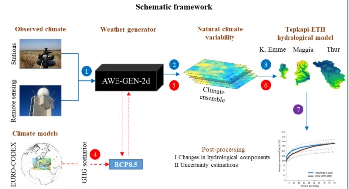
The general methodological framework of this project is illustrated in Figure 1. This illustrates the workflow that makes use of two state-of-the-art models, a high-resolution stochastic weather generator (AWE-GEN-2d) and a fully distributed hydrological model (Topkapi-ETH). AWE- GEN-2d was used to generate climate ensembles for the present and the future climate forced with the RCP8.5 emission scenario. Topkapi-ETH was used to estimate the changes in the future hydrological regimes and the associated uncertainties. The models and the details of the proce- dures that were applied are described in the following sections.
Figure 1 – A schematic representation of the methodological modelling framework. Points 1 to 7 are detailed de- scribed in Section 2.3.
2.1 THE AWE-GEN-2D MODEL
Weather generators (WGs) are numerical tools designed to produce synthetic time series of vari- ous meteorological variables of theoretically infinite length for a given climate and location.
Most of the existing WGs are designed for station-scale applications or as multi-station genera- tors and simulate climate variables at a daily or coarser temporal resolution (e.g. Keller et al., 2015). Gridded stochastic WGs are a suitable tool to generate multiple realizations of different climate variables at high spatial and temporal resolution while reproducing the spatial climate variability and the natural climate variability. Recently, a new stochastic weather generator model, the AWE-GEN-2d (Advanced WEather GENerator for a 2-dimensional grid), was pre- sented by Peleg et al. (2017). The model combines physical and stochastic approaches to simu- late key climate variables at high spatial and temporal resolution: 2 km x 2 km and 1 h for pre- cipitation and cloud cover and 100 m x 100 m and 1 h for near-surface air temperature, solar
radiation, vapor pressure, atmospheric pressure, and near-surface wind. The climate variables are auto- and cross-correlated in time and space. The WG is relatively parsimonious in terms of computational demand and allows the generation of multiple stochastic realizations in a fast and efficient way. Its performance was tested for small areas with a complex topography (Peleg et al., 2017, 2019; Skinner et al., 2020), as well as for larger domains (Peleg et al., 2020). The high- resolution climate variables reproduced by the WG can serve as inputs into distributed hydrolog- ical models. Moreover, AWE-GEN-2d is particularly suitable for studies where exploring cli- mate forcing uncertainty at multiple spatial and temporal scales is fundamental as the WG can be conveniently reparametrized to simulate different climates (Peleg et al., 2019).
2.2 TOPKAPI-ETHHYDROLOGICAL MODEL
A distributed investigation of the propagation of climate change effects on streamflow at fine spatial and temporal scales requires the use of a fully distributed hydrological model. The Topkapi-ETH model (Fatichi et al., 2015) used in this study is an advanced version of the TOpo- graphic Kinematic APproximation and Integration model (Topkapi; Todini and Ciarapica, 2001, Ciarapica and Todini, 2002). Among other applications, the model was used to investigate cli- mate change effects on the hydrology of the Po and Rhone river basins (Fatichi et al., 2014, Fatichi et al. 2015), and of the Kl. Emme (Battista et al., 2020; Paschalis et al., 2014). The model uses a grid-based representation of topography and a vertical discretization of the subsurface in three layers. The first two layers represent shallow and deep soil horizons and are schematized as non-linear reservoirs following the integration of the kinematic approximation of the momentum and mass conservation equations, whereas the third layer is schematized as a linear reservoir use- ful to mimic the behaviour of slow-flow components such as porous or fractured rock aquifers.
Grid elements are connected in the surface and the subsurface according to topographic gradi- ents. The model simulates surface and subsurface flow while considering processes as intercep- tion, infiltration, evapotranspiration, and snow and ice melt over each grid cell. Topkapi-ETH represents a reasonable compromise between the fully physically-based meaningful representa- tion of hydrological processes and computational time for large scales (>1,000 km2), long-term (>20 y), high-resolution (<1 km2, hourly) distributed simulations in a stochastic framework. In the context of this study it is worth to mention that it can preserve relatively high-resolution to- pography, which is an important asset for hydrological simulations in complex terrain.
2.3 FROM CLIMATE TO HYDROLOGICAL PREDICTIONS
The methodological modelling framework of this study required to carry out seven steps, illus- trated in Fig. 1, to estimate the changes in the hydrological components for the future climate.
First, the AWE-GEN-2d model was used to simulate the ensembles of climate variables repre- senting the present climate (steps 1 and 2). Three ensembles were generated, one for each of the examined catchments. The methods for calibrating and validating the AWE-GEN-2d model are described in detail by Peleg et al. (2017). In step 1, data that were obtained from different sources (see Section 4) were analysed and processed to be used as input variables for the model.
In step 2, the climate ensembles representing the present period (1976-2005) were generated.
are stationary, i.e. no climate trends exist. The following climate variables were simulated: pre- cipitation, cloud cover, near-surface air temperature, relative humidity, and solar radiation. All variables were simulated over a grid, with a temporal resolution of 1 h and a spatial resolution of 2 km x 2 km.
The Topkapi-ETH model was calibrated for the three catchments using observed data of climate (precipitation, temperature and cloud cover) and streamflow (see Section 4). The model was cali- brated following a well-established calibration procedure that was used in past studies for vari- ous catchments in Switzerland (e.g. Fatichi et al., 2015; Pappas et al., 2015; Paschalis et al., 2014). After calibration, the present climate ensembles, simulated in steps 1 and 2, were used as input into Topkapi-ETH to simulate the hydrological flows at present climate conditions (step 3).
The simulated streamflow with AWE-GEN-2d data was compared with the observed streamflow to evaluate both models (AWE-GEN-2d and Topkapi-ETH) abilities in statistically reproducing the hydrology for the present climate.
Next, the AWE-GEN-2d model was re-parameterised to simulate climate ensembles for future climate conditions. To that end, 9 regional climate models (Section 4) from the EURO-
CORDEX project (quantile mapped following Rajczak et al. (2016) method as in CH2018), which simulate the future climate for the highest emission scenario path (RCP8.5), were used.
The parameters used to simulate precipitation and temperature in AWE-GEN-2d for the present climate were re-calibrated (step 4) to follow the statistics of the future climate by applying a fac- tor of change method on a seasonal basis (e.g. Fatichi et al., 2011). Future climate ensembles were then generated for each of the catchments (step 5). A 30-year ‘moving window’ technique was used to generate continuous precipitation and temperature series for the period between 2020 and 2099 (Peleg et al., 2019). The ensembles generated for the future climate consist of 10 realizations of 10 years each, for each decade and regional climate model. In total 21,600 years were simulated (3 x 9 x 10 x 10 x 8; #catchment-ensemble, #climate-models, #realizations,
#members, #decades). The future climate ensembles were then used as input into Topkapi-ETH to simulate the hydrological flows for the future (step 6).
Last, the impacts of climate change on the hydrology were examined (step 7). The post-pro- cessing stage includes an assessment of the median and variability changes in the hydrological regime that were projected for each of the catchments and each of the climate trajectories (i.e. for each climate model). The stochastic variability was quantified by the 5-95th percentile range of the simulated, either climatic or hydrological, variable (as in Peleg et al., 2017, 2019). In addi- tion to the stochastic uncertainty, the hydrological uncertainty emerging from the various re- gional climate models was computed. To obtain a detailed analysis of the impact on the hydro- logical processes, we analysed the changes in seasonal streamflow, annual high and low flows, evapotranspiration, soil moisture and flow contribution from snow/ice melt.
3 STUDY CATCHMENTS
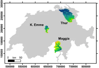
Three catchments representative of basin characteristics frequently found in Switzerland were chosen for this project: the Thur, Maggia and Kl. Emme (Figure 2). The catchments are charac- terised by a very heterogeneous spatial precipitation distribution, complex terrain and different size. The rationale for their selection was to favour catchments with minimum anthropogenic
influences, in the cases of Kl. Emme and Thur, and with a high degree of impounding for hydro- power production, in the case of Maggia.
Thur catchment. The catchment is located in the north-eastern part of Switzerland (latitude, 47.4° N, longitude, 9.1° E, at catchment centre-point). It is a tributary of the Rhine, with a total drained area of 1,730 km2 and an elevation range between 359 and 2,434 m and mean elevation of 773 m. Precipitation averaged over the entire catchment for the present climate is
1,350 mm y-1. There are neither reservoirs nor lakes in the catchment.
Maggia catchment. The catchment is located in the southern part of Switzerland (46.3° N, 8.6°
E), and a small part of it belongs to Italy. It outflows into Lago Maggiore, with a total drained area of 840 km2 and an elevation range between 204 and 3,208 m with a mean of 1,532 m. Pre- cipitation averaged over the entire catchment for the present climate is 1,840 mm y-1. There are several reservoirs in the catchment, which makes the analysis of the impact of climate change on hydropower production interesting. Moreover, this region is climatologically prone to floods that are characterised by higher specific discharges because of the southern climatological regime, which is influenced by the Mediterranean cyclogeneses, and is thus of particular interest with re- spect to future climate response.
Kl. Emme catchment. The catchment is located in central Switzerland (46.9° N, 8° E). It has a total drained area of 477 km2 and an elevation range between 600 and 2,275 m with a mean of 1,172 m. The precipitation average over the entire catchment for the present climate is
1,800 mm y-1. The catchment is glacier free and mostly covered by natural vegetation, except for small cropland areas and villages. The river flow regime is close to natural conditions without any major withdrawals for irrigation or hydropower uses.
Figure 2 – Location map of the catchments. Coordinates are in Swiss projection (CH-1903) in m.
4 DATA
Present climate. Climate data (precipitation, temperature, and radiation) were obtained from the Swiss Federal Office for Meteorology and Climatology (MeteoSwiss) from three different sources: ground stations (summarized in Table 1), weather radar system (Gabella et al., 2005;
Germann et al., 2006) and grid-data products (RhiresD - Schwarb, 2000 and TabsY - Frei, 2014).
Cloud cover data and wind speed at 500 hPa level were obtained from the MERRA-2 reanalysis product (Gelaro et al., 2017) and aerosols optical depth were calculated based on data derived from the AERONET network (Holben et al., 1998).
Future climate. Nine regional climate models were chosen from the CH2018 archive to be used in this project (Table 2). The climate models are part of the EURO-CORDEX initiative (Jacob et al., 2014). The original simulations were performed at a spatial resolution of 12.5 km ´ 12.5 km.
The climate model outputs were processed within the CH2018 project, quantile mapped and re- gridded for the Switzerland domain at 2 km ´ 2 km resolution.
Streamflow data. Hourly and daily streamflow estimates for gauged locations within the three catchments were obtained from BAFU archives (Table 3).
Table 1 – List of ground stations from MeteoSwiss.
Catchment Station name
Maggia
Cimetta
Acquarossa / Comprovasco Piotta
Robiei Ulrichen
Cavergno Bignasco Camedo
Osservatorio Ticinese Locarno
Thur
Ebnat-Kappel Güttingen Oberriet Säntis Schaffhausen St. Gallen Aadorf / Tänikon Vaduz
Wädenswil
Kl. Emme
Luzern Napf Pilatus
Table 2 – List of climate models from the CH2018 archive that were used in this project.
ID RCM Driving GCM
1 CLMcom-CCLM4-8-17 ICHEC-EC-EARTH
2 DMI-HIRHAM5 ICHEC-EC-EARTH
3 SMHI-RCA4 ICHEC-EC-EARTH
4 CLMcom-CCLM4-8-17 MOHC-HadGEM2-ES
5 SMHI-RCA4 MOHC-HadGEM2-ES
6 SMHI-RCA4 IPSL-IPSL-CM5A-MR
7 CLMcom-CCLM4-8-17 MPI-M-MPI-ESM-LR 8 MPI-CSC-REMO2009 MPI-M-MPI-ESM-LR
9 SMHI-RCA4 MPI-M-MPI-ESM-LR
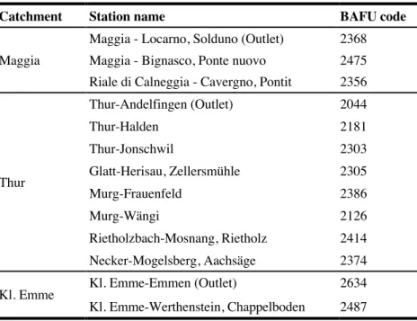
Table 3 – List of streamflow recording stations that were used in this project.
Catchment Station name BAFU code
Maggia
Maggia - Locarno, Solduno (Outlet) 2368 Maggia - Bignasco, Ponte nuovo 2475 Riale di Calneggia - Cavergno, Pontit 2356
Thur
Thur-Andelfingen (Outlet) 2044
Thur-Halden 2181
Thur-Jonschwil 2303
Glatt-Herisau, Zellersmühle 2305
Murg-Frauenfeld 2386
Murg-Wängi 2126
Rietholzbach-Mosnang, Rietholz 2414 Necker-Mogelsberg, Aachsäge 2374
Kl. Emme Kl. Emme-Emmen (Outlet) 2634
Kl. Emme-Werthenstein, Chappelboden 2487
5 RESULTS
Results of the validation of the weather generator model and the hydrological model are pre- sented first, followed by the results of the changes in climate and hydrology.
5.1 VALIDATION OF AWE-GEN-2D
The AWE-GEN-2d model was validated for reproducing the climate variables needed for the hy- drological simulations (e.g. precipitation, near-surface air temperature, cloud cover, and radia- tion) in the three catchments, following the same validation procedure introduced by Peleg et al.
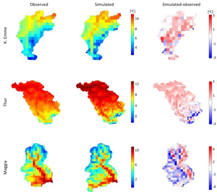
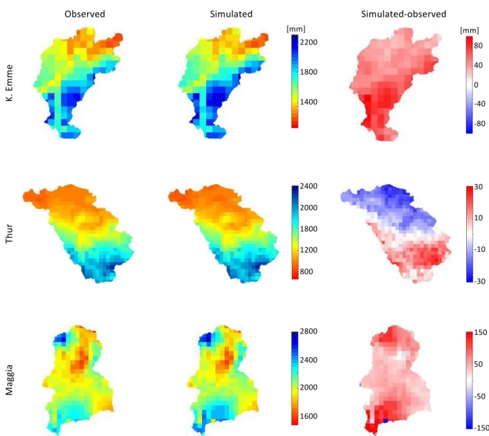
catchments. Most grid cells in the Kl. Emme show a difference between observed and simulated temperatures that are smaller than 1°C. The same holds for the Thur catchment, where most grid cells show an overestimation of the simulated temperature by up to 1 °C, except for the high mountainous region in the south-east where the model produces an underestimation of the tem- perature by up to 3°C. The differences between observed and simulated temperature in the Mag- gia catchment are much higher than in the other two catchments, reaching up to ±6 °C differ- ence. However, it seems that there is a shift of 2-4 km along the east-west axis in the location of the valley and mountains between the observed and simulated maps that may be the source of this apparent error.
Figure 4 compares the annually averaged precipitation maps. Precipitation is well captured in the Kl. Emme catchment. The comparison may suggest an overestimation of model outputs over the catchment, but the maximum deviation is in the order of 4%, which compares well with the ex- pected natural variability of precipitation for this region (Fatichi et al., 2016a; Peleg et al., 2017).
In the Thur catchment, the model underestimates precipitation in the north of the catchment (low elevation region) and overestimates precipitation in the southern (mountainous) part of the catch- ment. Yet, the under/overestimation is also in this case very small, in the order of 3%. In the Maggia catchment, the model generally overestimates precipitation (up to 9%), except for a sin- gle grid cell where underestimation is recorded (of 8%). We note that the area in the south-west of the catchment lies outside of Switzerland border, thus precipitation is estimated using other product then RhiresD.
Temperature and precipitation were also validated at sub-daily (hourly) and seasonal scales. This was done using observed data from climate stations that are located within or near the borders of the catchments. Here, we present the validation using a single climate station for each of the catchments. The observed and simulated diurnal cycle of temperature is presented in Figure 5.
For all locations, the timing of the maximum and minimum daily temperatures and the diurnal dynamics are well simulated. The largest offset in hourly temperature in the Kl. Emme is less than 0.5 °C. The largest difference between observed and simulated hourly temperature in the Thur catchment is in the order of 1.3 °C, which is still within an acceptable range. In the Maggia catchment, the model overestimates the hourly maximum peak temperature and underestimates the minimum daily hourly temperature by up to 2 °C.
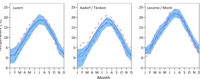
The model captures the seasonal dynamics of temperature well for all three catchments (Figure 6). The model overestimates summer temperatures in the Thur catchment (up to 2 °C) and in the Maggia catchment (up to 0.5 °C). We note that differences in temperature in the order of few °C are acceptable as they are within the error in monthly temperature estimation that depends on the sample size (i.e. the number of years/months).
The model's abilities to reproduce the seasonal dynamics were also explored for precipitation (Figure 7). The monthly mean precipitation and the natural variability in precipitation (presented using the 5-95th percentile range) are simulated well in the Kl. Emme and Maggia catchments but overestimated for the winter period (by up to 35 mm) on Thur.
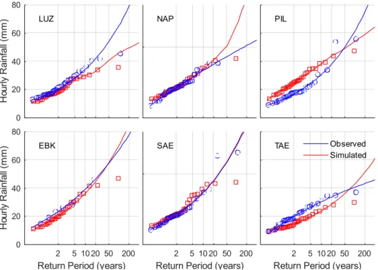
Finally, Figure 8 illustrates the model abilities to reproduce extreme precipitation at the hourly scale. The model was not calibrated to simulate extreme precipitation at sub-daily scales explic- itly (calibration was done on daily estimates). Yet, a good fit is achieved between the observed
and simulated extremes for most locations, especially between the 1 and 30 years return periods (for which records are available). In the Kl. Emme a small overestimation of the extreme precipi- tation intensity is detected at some of the locations where observations are available, while a small underestimation is found for several locations in the Thur catchment. We note, however, that the uncertainty in the observed gridded estimates obtained from MeteoSwiss is high (Scherrer et al., 2016).
Figure 3 – Mean near-surface air temperature for the period 1982-2015 as obtained from the TabsY product (ob- served) in comparison with the mean ensemble generated by AWE-GEN-2d (simulated).
Figure 4 – Mean precipitation for the period 1982-2015 as obtained from the RhiresD product (observed) in compar- ison with the mean ensemble generated by AWE-GEN-2d (simulated).
Figure 5 – Observed mean diurnal cycle of temperature (blue) and simulated (red) computed from the generated cli- mate ensemble. Location: Luzern – Kl. Emme, Aadorf – Thur, and Locarno – Maggia.
Figure 6 – A comparison between observed and simulated temperatures for each month. The blue and red solid lines represent the observed and simulated median values (respectively) and the bounded areas represent the observed (blue area) and simulated (dashed lines) 5–95th percentile range (respectively). The observed period covers 34 years of data (1982–2015), while simulations represent the mean of 30 realizations of 30 years each.
Figure 7 – A comparison between observed and simulated precipitation for each month. The blue and red solid lines represent the observed and simulated median values (respectively) and the bounded areas represent the observed (blue area) and simulated (dashed lines) 5–95th percentile range (respectively). The observed period covers 34 years of data (1982–2015), while simulations represent the mean of 30 realizations of 30 years each.
Figure 8 – Validation of annual maximum precipitation intensity at the hourly scale for different return periods in the Kl. Emme (top row) and Thur (bottom row) weather stations. The solid lines represent the observed (blue) and simulated (red) precipitation intensity computed by fitting GEV distribution to the data. The observed period covers 34 years of data (1982–2015), while simulations represent the mean of 30 realizations of 30 years each.
5.2 VALIDATION OF TOPKAPI-ETH
The Kl. Emme and Thur catchments are considered as natural catchments, i.e. their streamflow is not altered by regulated by infrastructures and/or human activities, so that the model perfor- mance at the outlet of the catchment could be evaluated against observed data. The Maggia catchment is completely regulated due to the hydropower operation, and thus the model was evaluated against the flow into the hydropower reservoirs instead, which are considered as a nat- ural flow (Figure 9).
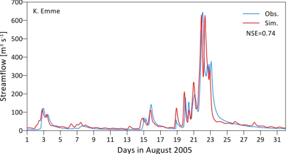
Topkapi-ETH was validated at the hourly and monthly scales on available streamflow observa- tions. First, a Nash–Sutcliffe Efficiency index (NSE) was computed for the period between 2000 and 2009 at the hourly scale, yielding values of 0.74 for the Kl. Emme catchment and 0.57 for the Thur catchment. An example of Topkapi-ETH simulation is presented in Figure 10.
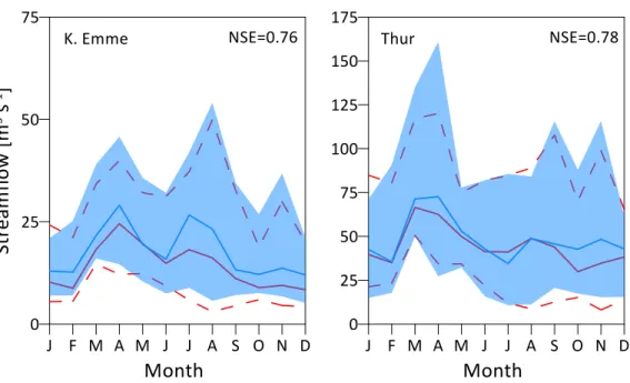
At the monthly scale (Figure 11), the model preserves the high NSE values (0.76 and 0.78 for the Kl. Emme and Thur catchments, respectively), but underestimates mean monthly flows for most of the months in the Kl. Emme catchment (up to 30%) and for October-November months in the Thur catchment (up to 20%). However, the model correctly reproduces the seasonal dynamics and the natural variability of streamflow. Examining longer periods (i.e. extending the compari- son beyond the years used for the calibration of the model), confirms the monthly NSE values of 0.74 for the Kl. Emme (1986-2009) and 0.76 for the Thur (1982-2009) catchments.
2 5 10 20 50 200 Return Period (years) 0
20 40 60 80
Hourly Rainfall (mm) LUZ
2 5 10 20 50 200 Return Period (years)
NAP
2 5 10 20 50 200 Return Period (years)
PIL
2 5 10 20 50 200 Return Period (years) 0
20 40 60 80
Hourly Rainfall (mm) EBK
2 5 10 20 50 200 Return Period (years)
SAE
2 5 10 20 50 200 Return Period (years)
TAE Observed
Simulated
In addition to the NSE score, the model simulations were evaluated against the maximum annual streamflow observed at the outlets of the Kl. Emme and Thur catchments (Figure 12). The model captures the hourly streamflow extremes for the return periods between 1 and 30 years well but underestimates the low-frequency streamflow extremes in Thur while overestimating the low- frequency streamflow extremes (i.e. above the 100-year return period) in the Kl. Emme. As for the precipitation extremes, the observed data is characterized by high uncertainties (Hilker et al., 2009), which are of the same order of magnitude of the confidence intervals presented in Figure 12.
Figure 9 – A comparison between observed and simulated inflow for each month (2006-2015, excluding 2010) in Sambuco reservoir. The blue and red lines represent the observed and simulated mean values (respectively).
Figure 10 – A comparison between observed (blue) and Topkapi-ETH simulated (red) streamflow (outlet of Kl.
Emme catchment). NSE refers to the Nash–Sutcliffe efficiency that was computed at the hourly scale for the pe- riod 2000-2009.
Figure 11 – A comparison between observed and simulated streamflow for each month (2000-2009). The blue and red solid lines represent the observed and simulated median values (respectively) and the bounded areas repre- sent the observed (blue area) and simulated (dashed lines) 5–95th percentile range (respectively).
Figure 12 – Comparison between observed and simulated peak-over-threshold at the hourly scale for different return periods in the Kl. Emme (left) Thur (right) catchments. The solid lines represent the observed (blue) and simu- lated (red) streamflow computed by fitting a Generalized Pareto distribution to the recorded data for the 2000–
2009 period. The plotting positions were calculated using Gringorten’s equation and the return periods are calcu- lated via the reduced variate method.
2 5 10 20 100 400 Return Period (years) 0
500 1000 1500
Flow (m3 /s) Kleine Emme Threshold=200m3/s
Observations Calibration
Calibration - Confidence Interval
2 5 10 20 100 400 Return Period (years) 0
500 1000 1500
Flow (m3 /s) Thur
Threshold=250m3/s Observations Calibration
Calibration - Confidence Interval