Testing in nonstationary and dependent panels with applications to purchasing power parity

Dependent Panels with Applications to

Purchasing Power Parity

Inauguraldissertation zur Erlangung des akademischen Grades

Doctor rerum politicarum der Universit¨ at Dortmund

Christoph Hanck

Februar 2007

Contents i

List of Figures iv

List of Tables vi

Preface vii

1 Introduction 1

2 Cointegration Tests of PPP: Do They Exhibit Erratic Be-

haviour? 9

2.1 Introduction . . . . 10

2.2 The PPP Condition . . . . 11

2.3 Cointegration Tests of PPP . . . . 12

2.4 Conclusion . . . . 22

3 A Meta Analytic Approach to Testing for Panel Cointegration 25 3.1 Introduction . . . . 26

3.2 P -Value Combination Tests for Panel Cointegration . . . . 26

3.3 Finite Sample Performance . . . . 32

3.4 Conclusion . . . . 41

i

4 Cross-Sectional Correlation Robust Tests for Panel Cointe-

gration 43

4.1 Introduction . . . . 44

4.2 P -Value Combination Tests for Panel Cointegration . . . . 46

4.3 Allowing for cross-sectional error dependence . . . . 51

4.4 A Monte Carlo study . . . . 55

4.5 An Empirical Test of the PPP Hypothesis . . . . 60

4.6 Conclusion . . . . 62

5 Are PPP Tests Erratic? Some Panel Evidence 65 5.1 Introduction . . . . 66

5.2 The Panel Tests . . . . 67

5.3 Results . . . . 70

5.4 Conclusion . . . . 72

6 The Error-in-Rejection Probability of Meta-Analytic Panel Tests 75 6.1 The P-Value Combination Test . . . . 77

6.2 The Error-in-Rejection Probability of the Combination Test . . 78

6.3 Conclusion . . . . 84

7 Mixed Signals Among Panel Cointegration Tests 87 7.1 Introduction . . . . 88

7.2 Panel Cointegration Tests . . . . 89

7.3 Do Panel Cointegration Tests Produce “Mixed Signals”? . . . . 93

7.4 Conclusion . . . 100

8 For Which Countries did PPP hold? A Multiple Testing

Approach 101

8.1 Introduction . . . 102

8.2 The Multiple Testing Approach . . . 104

8.3 The Bootstrap Algorithm . . . 107

8.4 Results . . . 109

8.5 Conclusion . . . 111

9 OLS-based Estimation of the Disturbance Variance under Spatial Autocorrelation 113 9.1 Introduction . . . 114

9.2 The relative bias of s

in finite samples . . . 117

9.3 Asymptotic bias and consistency . . . 120

10 Concluding Remarks 123

Bibliography 125

2.1 CPI-based Argentine t-stat series using a data-dependent lag choice

rule . . . . 16

2.2 CPI-based Finnish t-stat series using a data-dependent lag choice rule . . . . 16

2.3 CPI-based Mexican t-stat series using a data-dependent lag choice rule . . . . 17

2.4 CPI-based Chilean t-stat series using a data-dependent lag choice rule . . . . 17

2.5 CPI-based Danish t-stat series using a data-dependent lag choice rule 18 2.6 CPI-based Danish t-stat series with a moving window of T

= 30 . 19 2.7 WPI-based Argentine t-stat series using a data-dependent lag choice rule . . . . 19

2.8 WPI-based Danish t-stat series using a data-dependent lag choice rule . . . . 20

2.9 CPI-based Argentine t-stat series using 1 lag in ADF regression . . 20

2.10 CPI-based Argentine t-stat series using 2 lags in ADF regression . . 21

2.11 CPI-based Argentine t-stat series using 3 lags in ADF regression . . 21

2.12 CPI-based Argentine t-stat series using 4 lags in ADF regression . . 22

2.13 CPI-based Argentine ˆ λ-trace stat series . . . . 24

3.1 Power of the P panel cointegration tests . . . . 37

5.1 Test statistic series for L

for various N . . . . 71

5.2 Test statistic series for P

for various N . . . . 72

iv

5.3 Test statistic series for Z for various N . . . . 73

5.4 Test statistic series for P for various N . . . . 74

6.1 The density functions for the case N = 2 . . . . 82

6.2 Rejection Rates of P

test at 5% as a Function of N . . . . 83

6.3 Rejection Rates of P

test at 5% for differing degrees of “oversized- ness” . . . . 84

7.1 Correlation of Empirical p-values . . . . 97

9.1 The relative bias of s

as a function of ρ and N . . . 119

2.1 ADF Unit Root Tests . . . . 13

2.2 Successive t-stat results . . . . 15

2.3 Successive ˆ λ-test results . . . . 23

3.1 Empirical Size of the P Tests . . . . 34

3.2 Empirical Power of the P Tests . . . . 36

3.3 Power with AR(p) Errors . . . . 40

4.1 Rejection Rates of the P Tests. . . . 58

4.2 Tests for Weak Purchasing Power Parity . . . . 61

6.1 Simulated Type I Error Rates for the P

Test. . . . . 79

7.1 Correlation of the Empirical p-values under the Null . . . . 98

7.2 Fraction of joint rejections under H

and H

. . . . 99

8.1 Empirical Results . . . 109

vi

The following chapters present a synthesis of my research under the supervision of Walter Kr¨ amer and Kornelius Kraft during the past 18 months. It has been a pleasure to work under their fine guidance.

Many additional people have been a source of encouragement, providing helpful conversation, thoughtful advice and valuable feedback. I sincerely appreciated all of these, and have tried to follow most. Thanks go to my fellow doctoral students at the Ruhr Graduate School, to my colleagues and to Heide Aßhoff at the Institut f¨ ur Wirtschafts- und Sozialstatistik, Universit¨ at Dortmund. Spe- cial thanks are given at the beginning of the respective chapters to which they contributed in some way or another. It has been a pleasure to co-author chap- ters with Walter Kr¨ amer and Guglielmo Maria Caporale.

I am grateful for the efforts of my teachers at the doctoral program of the Ruhr Graduate School which both shaped my research and helped me become a more versatile economist. It is a pleasure to acknowledge the generosity of the Ruhr Graduate School through a research grant and funding of several presentations at international conferences. Both were instrumental in producing this thesis.

I am indebted to my parents for many things, but for the present purposes, I want to say that I would not have written this thesis had they not reared me as an (I think) inquiring mind. Finally, I thank Steffi for being and making me cheerful throughout. This would not have been possible without her.

vii

Introduction

The present dissertation aims to make a contribution to improved econo- metric practice in testing statistical hypotheses on nonstationary and (cross- sectionally) dependent panel datasets. I have chosen to illustrate the challenges involved in testing in nonstationary and dependent panels by focusing on the Purchasing Power Parity (henceforth, PPP) Condition, or Law of One Price, one of the most intensively discussed theories in international economics. How- ever, nonstationarity and cross-sectional dependence are common features of many macroeconomic panels. Hence, I conjecture that many of the issues dis- cussed and methods suggested here may also be fruitfully applied to other macroeconometric questions, such as the Fisher relation or savings and invest- ment correlations.

This Introduction briefly outlines the main results of and the common thread of the different chapters. These chapters are mainly taken from eight self- contained essays I have written (three of them together with Walter Kr¨ amer and Guglielmo Maria Caporale). I therefore have to beg the reader’s pardon for some redundancies, which, however, were inevitable to make each of the papers as coherent as possible.

Chapter 2, written together with Guglielmo Maria Caporale, adopts a more tra-

1

ditional time series based framework to highlight drawbacks in testing for PPP by means of Engle and Granger (1987) or Johansen (1988) type cointegration tests on the exchange rate and home and foreign price levels. It has long been known that these tests suffer from problems such as low power (Haug, 1996), size distortion (Gonzalo, 1994) or excessive sensitivity to nuisance parameters (Kremers, Ericsson, and Dolado, 1992). Similarly, it is well-known that the outcome of tests for PPP are quite sensitive to, e.g., how one constructs the price variables (Coakley, Kellard, and Snaith, 2005). Chapter 2 adds to this lit- erature by demonstrating that existing popular time series based cointegration tests seem to be uninformative about PPP (or “erratic”) in that the conclusion of the test is highly sensitive to the sample period an investigator uses.

One of the remedies suggested in the literature to overcome these problems is to employ panel data—i.e., to pool observations on several units (here, coun- tries) over time—to conduct estimation and inference (see, e.g., Baltagi, 2001).

Several panel unit root and cointegration tests and estimators (see Breitung and Pesaran, 2007, for a recent survey) have been developed to this end. The contribution of Chapter 3 is to provide some new tests for panel cointegration.

I extend the meta analytic panel unit root tests of Maddala and Wu (1999) and Choi (2001) to the cointegration setting. Compared with other tests in the literature, the meta analytic approach has the advantage of being highly flexible, relatively easy to implement and quite intuitive. I conduct a simula- tion study to demonstrate that several variants of the new tests compare quite favorably with existing ones in terms of both type I and type II error rates.

The tests put forward in Chapter 3 belong to the class of so called “First-

Generation Tests” in that they ignore the potential presence of cross-sectional

dependence among the countries in the panel. This is of course easily seen

to be a very restrictive assumption (made to simplify the derivation of the

asymptotic distribution of the tests). To give an example, it is tantamount

to assuming that the exchange rate behaviour of the British Pound to the U.S. dollar is independent of the exchange rate behaviour of the Euro to the Dollar.

Recent work—so called “Second-Generation Tests” (e.g., Bai and Ng, 2004;

Phillips and Sul, 2003)—has therefore focused on relaxing this assumption.

Chapter 4 builds on Chapter 3 in that the most promising variants of the meta analytic panel tests are used to provide additional cross-sectional correlation robust tests for panel cointegration. I employ a sieve bootstrap approach to account for nonstationarity and dependence under the maintained null hypoth- esis of no panel cointegration. This semi-parametric bootstrap scheme allows for more general forms of cross-sectional dependence than other robust tests previously suggested in the literature. Again, a simulation study reveals that the tests are capable of handling dependence of a quite general form. An em- pirical application to the PPP condition shows that properly accounting for the loss of information incurred by combining correlated rather than independent data weakens the evidence in favor of PPP.

Chapter 5, written together with Guglielmo Maria Caporale, revisits the ques- tion of erratic behaviour of PPP test statistics. We use cross-sectional corre- lation robust panel unit root tests to test the PPP hypothesis over different sample periods. It turns out that the behaviour of the panel test statistics shows no evidence of erraticism. We therefore conjecture that panel tests are capable of not only alleviating the above-mentioned well-known problems of, e.g., low power but also the issue of erraticism discussed in Chapter 2 and in Caporale, Pittis, and Sakellis (2003).

The previous chapters contribute evidence that panel tests—if properly

designed—hold much promise to become a useful standard tool in macro-

econometric practice. The following three chapters, on the other hand, high-

light some open issues in the use of panel tests.

Chapter 6 provides an analytic framework to understand the puzzling finding of many simulation studies that the performance of meta-analytic panel tests deteriorates if one increases the number of units in the panel. (We measure per- formance by control of the type I error rate. That is, a test performs well if its rejection rate—when applied to repeated drawings of finite samples generated under the null—is close to the nominal one.) This is, a priori, rather counterin- tuitive because one would normally expect the performance to improve if more information becomes available. I demonstrate that this puzzle can be explained by seemingly negligible size distortions of the time series tests used to construct the meta-analytic panel test statistics. These distortions then “add up” when combining ever more units to yield an increasingly size-distorted panel test. In practice, it is therefore strongly recommended to use time series tests which carefully control the type I error rate. I propose to solve or at least alleviate this problem by using adjusted critical values which give a better approxima- tion to the finite sample distribution than the fixed (first-order) asymptotic critical values. In practice, adjusted critical values may be obtained via the response surface regression approach pioneered in the cointegration literature by MacKinnon (1991).

Chapter 7 compares results from test outcomes of several popular panel cointe- gration tests when applied to artificial data. The use of artificial data allows to control the Data Generating Process, such as to know whether a particular test decision is correct or not. It turns out that panel cointegration tests produce

“mixed signals”—just as time series cointegration tests do (Gregory, Haug, and Lomuto, 2004). That is, it frequently occurs that one tests produces a rather emphatic rejection of the null hypothesis while another one confirms the null—

even though both are applied to the same sample. Put differently, it is likely

that it will be possible to find at least one test that, as desired, confirms or

rejects any given hypothesis tested on some dataset. The likely explanation for

this is that panel cointegration tests (unlike classical Wald, Likelihood Ratio or Lagrange Multiplier tests, for which Berndt and Savin (1977) show that the “mixed signals” problem vanishes asymptotically) have different implicit alternatives. E.g., Johansen (1988) type tests look at the eigenvalues of some residual moment matrix, whereas Engle and Granger (1987) type tests rely on the mean reversion of a residual series. While the alternatives of both tests is taken to be “cointegration,” the mathematical characterization obviously differs substantially.

The recommendation for empirical practice therefore is to report results on preferably several panel cointegration tests to increase the confidence one can put into the rejection or non-rejection of some particular economic hypothesis, provided the test results agree.

Chapter 8, on a more general level, takes issue with popular approaches to testing for PPP and suggests a novel one. One popular, traditional strategy is to gather price and exchange rate data on several countries (relative to some reference country) and test for PPP in each by, e.g., testing the null of a unit root in the real exchange rate. It is then argued that PPP holds for those countries for which the null of a unit root is rejected at, say, the 5%

level, because the real exchange rate is then statistically significantly mean- reverting. While this intuitive procedure is by construction adequate when one only considers a single country, it is questionable from a statistical point of view when applied to several countries simultaneously as it ignores the problem of multiplicity. That is, I demonstrate that one is almost bound to spuriously find some evidence in favor of PPP even if it is not present in any country because testing at, e.g., the 5% level in several countries does not control the type I error at the 5% level for the entire panel of countries.

Similarly, the panel approaches discussed in some of the previous chapters are

to be used with caution, too, as many of the available tests’ alternatives might

lead one to mistakenly believe PPP to hold for all countries in case of a rejection even if in fact it only holds for some. Moreover, existing panel tests do not allow to identify the countries for which PPP holds.

I therefore modify a recent proposal of Romano and Wolf (2005) to be appli- cable to the nonstationary testing problem. The main idea is to control for multiplicity with a multiple testing technique which, unlike traditional Bonfer- roni type multiple tests, guarantees high power of the procedure by exploiting the dependence structure among the countries with a bootstrap procedure. In- deed, my empirical results show that the modified Romano and Wolf (2005) approach seems to be more powerful than traditional multiple testing tech- niques in that it identifies PPP to hold for more countries. Conversely, the results suggest that the simple testing approach ignoring multiplicity as well as panel tests apparently produce spurious rejections which do not result if one properly accounts for multiplicity.

Finally, Chapter 9 adopts an alternative approach to model cross-sectional dependence. This chapter contributes to the spatial econometrics literature, where one proceeds by assuming a known form of cross-sectional dependence.

This assumption can be a plausible one if one can correctly capture the depen- dence structure among panels by observables as, e.g., trade shares. Consistent estimation is then possible even if only one panel wave is available.

The chapter first shows that the standard estimator of the disturbance variance,

i.e., the degrees of freedom adjusted mean of the sum of squared Ordinary

Least Squares (OLS) residuals, is applicable by demonstrating that the variance

covariance matrix of the reduced form errors of a spatial model is homoskedastic

under many popular specifications of the dependence structure. This clarifies

a recurrent misunderstanding in the literature. Then, the chapter derives the

exact finite sample bias of this estimator and proves its consistency. Hence,

it is shown that a simple and readily computed estimator can be used as an

ingredient in test statistics without affecting the asymptotic validity of the

tests.

Cointegration Tests Of PPP: Do They Exhibit Erratic

Behaviour?

Abstract

We analyse whether tests of PPP exhibit erratic behaviour (as previ- ously reported by Caporale, Pittis, and Sakellis, 2003) even when (pos- sibly unwarranted) homogeneity and proportionality restrictions are not imposed, and trivariate cointegration (stage-three) tests between the nominal exchange rate, domestic and foreign price levels are carried out (instead of stationarity tests on the real exchange rate, as in stage-two tests). We examine the US dollar real exchange rate vis-` a-vis 21 other currencies over a period of more than a century, and find that stage- three tests produce similar results to those for stage-two tests, namely the former also behave erratically. This confirms that neither of these traditional approaches to testing for PPP can solve the issue of PPP.

Keywords : Purchasing Power Parity (PPP), Real Exchange Rate, Coin- tegration, Stationarity, Parameter Instability

1

This chapter has been written jointly with Guglielmo Maria Caporale.

9

2.1 Introduction

Purchasing Power Parity (PPP) is one of the most popular theories for ex- plaining the long-run behaviour of exchange rates, and has therefore been ex- tensively investigated. Froot and Rogoff (1995) distinguish three stages in the time series literature on PPP. Stage-one tests were flawed by their failure to take into account possible non-stationarities in the series of interest. Stage-two tests focused on the null that the real exchange rate follows a random walk, the alternative being that PPP holds in the long run. However, such unit root tests were found to have very low power, and not to be able to distinguish between random-walk behaviour and very slow mean-reversion in the PPP- consistent level of the real exchange rate (see, e.g., Frankel, 1986, and Lothian and Taylor, 1997), unless very long spans of data were used (see, e.g., Lothian and Taylor, 1996, and Cheung and Lai, 1994).

Stage-three tests have used cointegration tests, but essentially suffer from the same problem of low power, and consequently have not significantly improved our understanding of real exchange rate behaviour (see Rogoff, 1996).

Caporale, Pittis, and Sakellis (2003) aimed to find an explanation for the con- tradictory evidence on PPP, even when long runs of data are used to increase the power of test statistics. They focused on stage-two tests and argued that the reason is that the type of stationarity exhibited by the real exchange rate cannot be accommodated by the fixed-parameter autoregressive homoscedastic models normally employed in the literature. Using a dataset including 39 coun- tries and spanning a period of up to two centuries, they analysed the behaviour of both WPI- and CPI-based measures of the real exchange rate. In particular, they computed a recursive t-statistic (see below for a precise definition), and showed that it has an erratic behaviour, suggesting the presence of instability,

2

Indeed, Kr¨ amer and Marmol (2004) show that the divergence of Dickey-Fuller type unit

root tests is slower against slowly mean-reverting I(d) alternatives.

and of a type of non-stationarity more complex than the unit root one usually assumed.

In the present study we explore this issue further by analysing whether erratic behaviour also characterises stage-three tests. The advantage of such tests is that they do not impose the homogeneity and proportionality restrictions entailed by stage-two tests, which might not hold in practice. Therefore, by carrying out cointegration tests of PPP we check whether there might be a relation between the presence of erratic behaviour and the imposition of overly strong restrictions. The layout of the chapter is as follows. Section 2 reviews the PPP condition in its different forms. Section 3 describes the data and presents some empirical evidence based on two different cointegration methods. Section 4 summarises the main findings and offers some concluding remarks.

2.2 The PPP Condition

In its absolute form, the PPP condition states that the nominal exchange rate should be proportional to the ratio of the domestic to the foreign price level, i.e.:

s

= α + β

p

+ β

p

, (2.1) where s

is the nominal exchange rate, p

the domestic price level, and p

the foreign price level, all in logs.

This is known as a trivariate relationship.

Imposing the “symmetry” restriction β

= −β

= β on the price coefficients, one obtains the following bivariate relationship:

s

= α + β(p

− p

). (2.2) Finally, the “proportionality” restriction α = 0, β = 1 implies

q

= s

− p

+ p

, (2.3)

3

Relative PPP implies that the percentage change in the exchange rate between two

currencies equals the inflation differential, i.e. ∆s

= β

∆p

− β

∆p

.

where q

is the real exchange rate.

Most of the literature in the 1980s tested PPP by means of (stage-two) unit root tests (DF or ADF—see Dickey and Fuller, 1979) on the real exchange rate, which, under PPP, should revert to its long-run equilibrium value given by PPP after being hit by shocks. The null hypothesis is that it follows a random walk (it has a unit root), since market efficiency implies that its changes should be unpredictable, whilst the alternative is that PPP holds. The maintained (joint) hypothesis is that the symmetry/proportionality restrictions both hold, which might not be true in practice. Consequently, the evidence presented by Caporale, Pittis, and Sakellis (2003) on the erratic behaviour of unit root tests might reflect unwarranted restrictions.

By contrast, a trivariate cointegration test of PPP entails running the following cointegrating regression (which does not impose any such restrictions):

s

= α + β

p

− β

p

+ u

(2.4) where the variables are defined as before, and u

stands for the regression errors. PPP is then tested by means of DF and ADF tests on the estimated residuals. In the present chapter, by implementing cointegration tests of this type, we aim to establish whether or not evidence of erratic behaviour can still be found, even without the abovementioned restrictions, and consequently whether or not the findings of Caporale, Pittis, and Sakellis (2003) are robust or instead are due the imposition of unwarranted restrictions.

2.3 Cointegration Tests of PPP

Data sources and definitions

We revisit the dataset employed by Taylor (2002), which includes annual data

for the nominal exchange rate, CPI and the GDP deflator. This dataset is

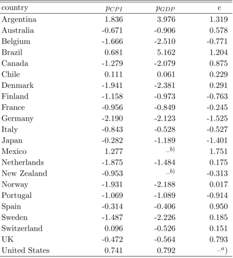
Table 2.1: ADF Unit Root Tests

country p

p

e

Argentina 1.836 3.976 1.319

Australia -0.671 -0.906 0.578

Belgium -1.666 -2.510 -0.771

Brazil 0.681 5.162 1.204

Canada -1.279 -2.079 0.875

Chile 0.111 0.061 0.229

Denmark -1.941 -2.381 0.291

Finland -1.158 -0.973 -0.763

France -0.956 -0.849 -0.245

Germany -2.190 -2.123 -1.525

Italy -0.843 -0.528 -0.527

Japan -0.282 -1.189 -1.401

Mexico 1.277 –

1.751

Netherlands -1.875 -1.484 0.175

New Zealand -0.953 –

-0.313

Norway -1.931 -2.188 0.017

Portugal -1.069 -1.089 -0.914

Spain -0.314 -0.406 0.950

Sweden -1.487 -2.226 0.185

Switzerland 0.096 -0.526 0.151

UK -0.472 -0.564 0.793

United States 0.741 0.792 –

)

N.A.:

) reference country

b

) series unavailable/too short

The number of lagged differences is chosen according to the MAIC (Ng and Perron, 2001). Yearly data from 1892 to 1996. p

is the log CPI price level, p

is the log GDP deflated price level and e is the log nominal exchange rate.

particularly useful for our purposes because it covers a long period, ranging

from 1892 through to 1996. The countries contained in our panel are given in

Table 2.1. We use the United States as the reference country throughout. See

Taylor (2002) for further details on data sources and definitions.

Empirical analysis

As a first step, we carried out standard augmented Dickey-Fuller (Said and Dickey, 1984) unit root tests to establish whether the series are all I (1), and it is therefore legitimate to test for cointegration. The results indicate that this hypothesis can indeed not be rejected (see Table 2.1). We then proceeded to the estimation of cointegrating regressions using the Engle and Granger (1987) methodology. That is, we estimated (2.4) by OLS, and used the residuals to test the null hypothesis that they are nonstationary (i.e., that PPP does not hold) by means of DF and ADF tests. In order to investigate possible parameter instability, we created a new time series “t-stat” which is the computed t- statistic from the successive estimation of the coefficients of the following model whose order is selected using the Modified AIC (MAIC) of Ng and Perron (2001):

∆ˆ u

= α

+ α

u ˆ

+

p

X

j=1

γ

∆ˆ u

+ ε

(2.5)

Here, ˆ u

are the residuals from OLS estimation of the cointegrating regression (2.4), ε

is a white noise error term, and t-stat is defined as ˆ α

/est.s.e.( ˆ α

).

Equation (2.4) is estimated using the first k observations to produce the first residual series, from which we compute the unit root test statistic ˆ α

/est.s.e.( ˆ α

).

We then add an extra observation to compute the second estimate based on k + 1 data points, and repeat the process until all T available observations have been used to yield T − k + 1 values of the test statistics. We let k ≈ 20 − 25 to discard estimates which are heavily affected by small-sample size-distortion.

One can then plot the t-statistics based on the successive estimates to see more

clearly whether it changes substantially as more data points are added, which

would be a strong indication of instability in the parameter. Big jumps in

either the rejection or the acceptance region, or from one to the other, are

a strong sign of a structural break in the DGP. The results are summarised

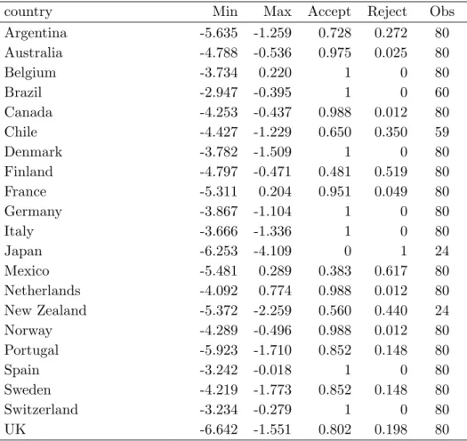
Table 2.2: Successive t-stat results

country Min Max Accept Reject Obs

Argentina -5.635 -1.259 0.728 0.272 80

Australia -4.788 -0.536 0.975 0.025 80

Belgium -3.734 0.220 1 0 80

Brazil -2.947 -0.395 1 0 60

Canada -4.253 -0.437 0.988 0.012 80

Chile -4.427 -1.229 0.650 0.350 59

Denmark -3.782 -1.509 1 0 80

Finland -4.797 -0.471 0.481 0.519 80

France -5.311 0.204 0.951 0.049 80

Germany -3.867 -1.104 1 0 80

Italy -3.666 -1.336 1 0 80

Japan -6.253 -4.109 0 1 24

Mexico -5.481 0.289 0.383 0.617 80

Netherlands -4.092 0.774 0.988 0.012 80

New Zealand -5.372 -2.259 0.560 0.440 24

Norway -4.289 -0.496 0.988 0.012 80

Portugal -5.923 -1.710 0.852 0.148 80

Spain -3.242 -0.018 1 0 80

Sweden -4.219 -1.773 0.852 0.148 80

Switzerland -3.234 -0.279 1 0 80

UK -6.642 -1.551 0.802 0.198 80

Minimum and maximum t-test statistics, acceptance and rejection percentages and number of available observations for each country, using CPI price series

in Table 2.2. Columns 4 and 5 show that the test decision on whether PPP holds or not is not constant over the sample in the vast majority of countries.

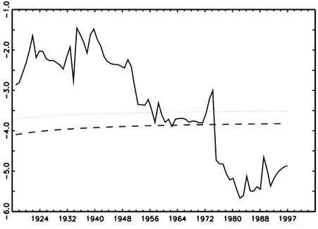
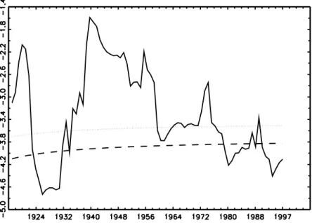
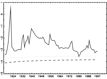
Frequent switches from the rejection to the non-rejection regions are found to occur, the successive t-statistic exhibiting erratic behaviour very similarly to the case of stage-two tests. For some graphical illustration, consider the cases of Argentina (Figure 2.1), Finland (Figure 2.2), Mexico (Figure 2.3), or Chile (Figure 2.4).

The instability found clearly does not concern specific points in time, such that it could be dealt with using procedures for cointegration testing in the presence of structural breaks (see, e.g., Hansen, 1992, or Gre-

4

The two lines at the bottom are the 10% and 5% critical values calculated as in

MacKinnon (1991).

Figure 2.1: CPI-based Argentine t-stat series using a data-dependent rule (Ng and Perron, 2001) for the choice of lags in the ADF regression

Figure 2.2: CPI-based Finnish t-stat series using a data-dependent rule (Ng and Perron, 2001) for the choice of lags in the ADF regression

gory and Hansen, 1996), but appears instead to be of an endemic type. As

a counterexample where no switches occur at the finite sample 5% level, see

Denmark (Figure 2.5).

Figure 2.3: CPI-based Mexican t-stat series using a data-dependent rule (Ng and Perron, 2001) for the choice of lags in the ADF regression

Figure 2.4: CPI-based Chilean t-stat series using a data-dependent rule (Ng and Perron, 2001) for the choice of lags in the ADF regression

We conducted the same type of analysis using the GDP deflator this time to

construct the real exchange rate, obtaining a very similar picture, namely er-

ratic behaviour in the majority of cases. For instance, compare Figure 2.7 with

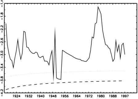
Figure 2.5: CPI-based Danish t-stat series using a data-dependent rule (Ng and Perron, 2001) for the choice of lags in the ADF regression

the corresponding CPI based Figure 2.1. There are only a few exceptions, such as Denmark, where no rejections occur (Figure 2.8).

Further, as a robustness check, we tried different number of lags in the ADF regressions (2.5). Over- all, a qualitatively similar pattern emerges throughout, although we find that higher number of lags are associated with fewer rejections (see Figure 2.1 and Figures 2.9 to 2.12). This is what one would expect, the estimation of too many parameters resulting in lower power (Phillips and Perron, 1988).

To explore more in depth the issue of possible structural breaks, we also used fixed-size windows.

That is, we select a fixed sample size T

and create the nth entry of the series t-stat as before but now based on observations t = n, . . . , T

+ n, where n = k, . . . , T − T

. One would expect using fixed windows to reduce the likelihood of structural breaks occurring within the chosen sample, and hence to result in more frequent rejections of the null hypothesis that PPP

5

Results for other countries are available upon request.

6

A variety of other methods could also be used to shed additional light on whether

structural breaks are present. See, e.g., Ploberger, Kr¨ amer, and Kontrus (1989).

Figure 2.6: CPI-based Danish t-stat series with a moving window of T

= 30

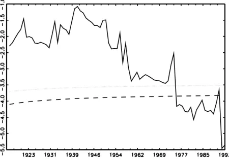
Figure 2.7: WPI-based Argentine t-stat series using a data-dependent rule (Ng and Perron, 2001) for the choice of lags in the ADF regression

does not hold. However, it turns out that the behaviour of the t-stat series

is, if anything, even more erratic than for increasing window sizes. It appears

that the answer to whether or not PPP holds is highly dependent on the chosen

sample. For instance, using Danish data ending in the 1960s and early 70s an

Figure 2.8: WPI-based Danish t-stat series using a data-dependent rule (Ng and Perron, 2001) for the choice of lags in the ADF regression

Figure 2.9: CPI-based Argentine t-stat series using 1 lag in ADF regression

investigator using T

= 30 years of data would strongly reject the null of PPP not holding (see Figure 2.6).

Finally, we carried out alternative cointegration tests in all cases. Specifically,

Figure 2.10: CPI-based Argentine t-stat series using 2 lags in ADF regression

Figure 2.11: CPI-based Argentine t-stat series using 3 lags in ADF regression

we used the λ-trace test (Johansen, 1988, 1991). Here the critical values were

obtained by modifying the asymptotic ones from Osterwald-Lenum (1992) us-

ing the response surface regression results of Cheung and Lai (1993). Some

Figure 2.12: CPI-based Argentine t-stat series using 4 lags in ADF regression

results are reported in Table 2.3.

Since this test statistic’s null distribution is related to the χ

distribution, unlike in the previous cases, the rejection region is now above the critical value lines. As can be seen, we find further evidence of erratic behaviour (Figure 2.13), suggesting that this is not due to the type of cointegration test used, but it is a more fundamental issue pertaining to the stochastic properties of the PPP relationship. Interestingly, switches from the rejection to the non-rejection region occur around the same time in a number of cases—compare, e.g., Figures 2.1 and 2.13.

2.4 Conclusion

In this chapter we have analysed whether tests of PPP exhibit erratic be- haviour (as previously reported by Caporale, Pittis, and Sakellis, 2003) even

7

Again, using WPI data or a different number of lagged differences in the Johansen procedure does not make a qualitative difference. Detailed results are available upon request.

8

Similar patterns emerge for Australia, Brazil, Canada, Denmark, Finland, France, Mex-

ico, the Netherlands, Norway, Portugal, Sweden and the UK, that is 14 out of 19 countries

for which the sample size is sufficiently large to make statistically meaningful statements.

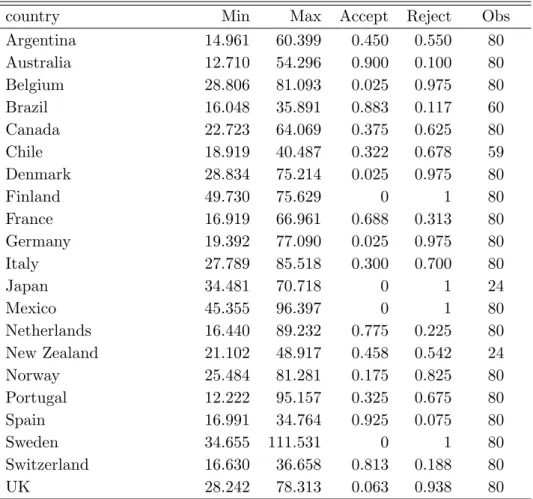
Table 2.3: Successive λ ˆ -test results

country Min Max Accept Reject Obs

Argentina 14.961 60.399 0.450 0.550 80

Australia 12.710 54.296 0.900 0.100 80

Belgium 28.806 81.093 0.025 0.975 80

Brazil 16.048 35.891 0.883 0.117 60

Canada 22.723 64.069 0.375 0.625 80

Chile 18.919 40.487 0.322 0.678 59

Denmark 28.834 75.214 0.025 0.975 80

Finland 49.730 75.629 0 1 80

France 16.919 66.961 0.688 0.313 80

Germany 19.392 77.090 0.025 0.975 80

Italy 27.789 85.518 0.300 0.700 80

Japan 34.481 70.718 0 1 24

Mexico 45.355 96.397 0 1 80

Netherlands 16.440 89.232 0.775 0.225 80

New Zealand 21.102 48.917 0.458 0.542 24

Norway 25.484 81.281 0.175 0.825 80

Portugal 12.222 95.157 0.325 0.675 80

Spain 16.991 34.764 0.925 0.075 80

Sweden 34.655 111.531 0 1 80

Switzerland 16.630 36.658 0.813 0.188 80

UK 28.242 78.313 0.063 0.938 80

Minimum and maximum ˆ λ-test statistics, acceptance and rejection percentages and number of available observations for each country, using CPI price series

when (possibly unwarranted) homogeneity and proportionality restrictions are not imposed, and trivariate cointegration (stage-three) tests between the nom- inal exchange rate, domestic and foreign price levels are carried out (instead of stationarity tests on the real exchange rate, as in stage-two tests). We ex- amine the US dollar real exchange rate vis-` a-vis 21 other currencies over a period of more than a century, and find that stage-three tests produce similar results to those for stage-two tests, namely the former also behave erratically.

This corroborates the findings of Caporale, Pittis, and Sakellis (2003), in the

sense that these do not appear to be the consequence of arbitrarily imposed

(symmetry/proportionality) restrictions.

Figure 2.13: CPI-based Argentine ˆ λ -trace stat series

Our results confirm that neither of the two traditional approaches to testing for

PPP (stage-two and stage-three tests) can solve the issue of PPP. Consistently

with Caporale, Pittis, and Sakellis (2003), the reported evidence again points to

some form of non-stationarity in the data which is unlike the standard unit-root

type normally assumed, or even the “separable” type discussed in Caporale and

Pittis (2002), but rather one where all the unconditional moments are unknown

functions of time. Future research should aim to determine its exact dynamic

features.

A Meta Analytic Approach to Testing for Panel Cointegration

Abstract

We propose new tests for panel cointegration by extending the panel unit root tests of Choi (2001) and Maddala and Wu (1999) to the panel cointegration case. The tests are flexible, intuitively appealing and rel- atively easy to compute. We investigate the finite sample behavior in a simulation study. Several variants of the tests compare favorably in terms of both size and power with other widely used panel cointegration tests.

Keywords : Panel cointegration tests, Monte Carlo study, Meta Analysis

25

3.1 Introduction

There is wide consensus in economics that cointegration is an important statis- tical concept which is implied by many economic models. In practice, however, evidence of cointegration or non-cointegration is often weak because of the rather small sample sizes typically available in macroeconometrics. To over- come this problem, the cointegration methodology has recently been extended to panel data. This allows the researcher to work with larger samples, thereby improving the power of tests and efficiency of estimators.

Pedroni (2004) and Kao (1999) generalize the residual-based tests of Engle and Granger (1987) and Phillips and Ouliaris (1990), Larsson, Lyhagen, and L¨ othgren (2001) extend the Johansen (1988) tests to panel data while Mc- Coskey and Kao (1998) propose a test for the null of panel cointegration in the spirit of Shin (1994).

The present chapter introduces some new tests for panel cointegration, extend- ing the p-value combination panel unit root tests of Maddala and Wu (1999) and Choi (2001) to the cointegration setting. In this framework, it is straight- forward to account for unbalanced panels and arbitrary heterogeneity in the serial correlation structure of the series. Moreover, the tests are simple to im- plement and intuitively appealing. We explore the finite sample performance of the new tests in a simulation study. Certain variants of the tests compare favorably with many previously proposed panel cointegration tests.

3.2 P -Value Combination Tests for Panel Cointegration

The present section develops the new tests for panel cointegration. The fol-

lowing notation is used throughout. x

is a (T

× 1) column vector collecting

the observations on the kth variable of unit i of the panel, where i = 1, . . . , N and k = 1, . . . , K. Additionally, we allow for time polynomials of order up to 2, i.e. constants, trend and squared trend terms. The number of observations T

per unit may depend on i, i.e. the panel may be unbalanced. Denote by p

the marginal significance level, or p-value, of a time series cointegration test applied to the ith unit of the panel. Let θ

be a time series cointegration test statistic on unit i for a sample size of T

. F

denotes the exact, finite T

null distribution function of θ

. Since the tests considered here are one-sided, p

= F

(θ

) if the test rejects for small values of θ

and p

= 1 − F

(θ

) if the test rejects for large values of θ

. We only consider time series tests with the null of no cointegration.

We are interested in testing the following null hypothesis

H

: There is no (within-unit) cointegration for any i, i = 1, . . . , N, (3.1) against the alternative

H

: There is (within-unit) cointegration for at least one i, i = 1, . . . , N.

The alternative H

states that a rejection is evidence of 1 to N cointegrated units in the panel. That is, a rejection neither allows to conclude that the entire panel is cointegrated nor does it provide information about the number of units of the panel that exhibit cointegrating relationships.

The main idea of the suggested testing principle has been used in meta analytic studies for a long time (cf. Fisher, 1970; Hedges and Olkin, 1985). Consider the testing problem on the panel as consisting of N testing problems for each unit of the panel. That is, conduct N separate time series cointegration tests and obtain the corresponding p-values of the test statistics.

We make the

1

Both Maddala and Wu (1999) and Choi (2001) suggest extending their panel unit root

tests to the cointegration case. However, to the best of our knowledge, they do not provide

an actual implementation nor do they investigate the performance of the tests. Furthermore,

our approach is more general and likely to be more accurate in some respects to be discussed

below.

following assumptions (see Pedroni, 2004).

Assumption 1 (Continuity)

Under H

, θ

has a continuous distribution function for all i = 1, . . . , N .

Assumption 2 (Cross-Sectional Uncorrelatedness)

x

= x

+ ξ

, t = 1, . . . , T

, i = 1, . . . , N, k = 1, . . . , K . Let ξ

≡ (ξ

, . . . , ξ

)

. We require E[ξ

ξ

] = 0 ∀ s, t = 1, . . . , T

and i 6= j. The error process ξ

is generated as a linear vector process ξ

= C

(L)η

, where L is the lag operator and C

are coefficient matrices. η

is vector white noise.

Remarks

• Assumption 1 is a regularity condition that asymptotically ensures a uniform p-value distribution of the time series test statistics under H

on the unit interval: p

∼ U [0, 1] (i ∈ N

) (see, e.g., Bickel and Doksum, 2001, Sec. 4.1). It is satisfied by the tests considered in this chapter.

• The second assumption is strong (see, e.g., Banerjee, Marcellino, and Osbat, 2005). It implies that the different units of a panel must not be linked to each other beyond relatively simple forms of correlation such as common time effects which can be eliminated by demeaning across the cross sectional dimension. This assumption is likely to be violated in many typical macroeconomic panel data sets. We will return to this issue in Chapter 4.

We now present the new tests. Combine the N p-values of the individual

time series cointegration tests, p

, i = 1, . . . , N , as follows to obtain three test

statistics for panel cointegration:

P

= −2

N

X

i=1

ln(p

) (3.2a)

P

= N

N

X

i=1

Φ

(p

) (3.2b)

P

= s

3(5N + 4) π

N (5N + 2)

N

X

i=1

ln p

1 − p

(3.2c) Here, Φ is the cdf of the standard normal distribution. When considered to- gether we refer to Eqs. (3.2a) to (3.2c) as P tests from now on. The P tests, via pooling p-values, provide convenient tests for panel cointegration by impos- ing minimal homogeneity restrictions on the panel. For instance, the different units of the panel can be unbalanced. Furthermore, the evidence for (non- )cointegration is first investigated for each unit of the panel and then com- pactly expressed with the p-value of the time series cointegration test. Hence, the coefficients describing the relationship between the different variables for each unit of the panel can be heterogeneous across i. Thus, the availability of large-T time series allows for pooling the data into a panel without having to impose strong homogeneity restrictions on the slope coefficients as in tradi- tional panel data analysis.

Under Assumptions 1 and 2, as T

→ ∞ for all i, the test statistics are asymptotically distributed as

P

→

χ

P

→

N (0, 1) P

→

T

,

where χ

is a chi-squared distributed random variable and T denotes Student’s t distribution. The subscripts give the degrees of freedom. Using consistent time series cointegration tests, p

→

0 under the alternative of cointegration.

Hence, quite intuitively, the smaller p

, the more it acts towards rejecting

2

For an overview of panel data models relying on N → ∞ asymptotics see Hsiao (2003).

the null of no panel cointegration. The decision rule therefore is to reject the null of no panel cointegration when P

exceeds the critical value from a χ

distribution at the desired significance level. For (3.2b) and (3.2c) one would reject for large negative values of the panel test statistics P

and P

, respectively.

We now discuss how to obtain the p-values required for computation of the P test statistics. (In Chapter 5, we will show that using accurate p-values for meta analytic panel tests is crucial to achieve a precise control of the type I error rate.) The null distributions of both residual and system-based time series cointegration tests converge to functionals of Brownian motion. Hence, analytic expressions of the distribution functions are hard to obtain, and p- values of the tests cannot simply be obtained by evaluating the corresponding cdf.

A remedy frequently adopted in the literature is to derive the critical values (and, consequently, the p-values) by Monte Carlo simulation. However, this approach is unsatisfactory for (at least) the following reason. These simulations are typically only performed for one sample size which is meant to provide an approximation to the asymptotic distribution. This sample size need neither be large enough to be useful as an asymptotic approximation nor does it generally yield accurate critical values for other sample sizes. MacKinnon, Haug, and Michelis (1999) show for cases where analytic expressions of the distribution functions are available that this approach may deliver fairly inaccurate critical values. In the time series case, it is now fairly standard practice to report p-values of unit root and cointegration tests using the results of the response surface regressions introduced by MacKinnon (1991). We follow this approach here.

The null hypothesis (3.1) formulates no precise econometric characterization

of (non-) cointegration. This is to allow for generality in testing the long-run

equilibrium properties of the series, enabling the researcher to use whichever time series tests seem suitable to test for time series (non-)cointegration in the different units of the panel. We use p-values of the Augmented Dickey- Fuller (ADF ) cointegration tests (Engle and Granger, 1987) as provided by MacKinnon (1996).

That is, the p-values are obtained from the t-statistic of γ

− 1 in the OLS regression

∆ˆ u

= (γ

− 1)ˆ u

+

P

X

p=1

ν

∆ˆ u

+

.

Here, ˆ u

is the usual residual from a first stage OLS regression of one of the x

on the remaining x

and, possibly, deterministic terms. Alternatively, one could capture serial correlation by the semiparametric approach of Phillips and Ouliaris (1990). Finally, we obtain the p-values for the Johansen (1988) λ

and λ

tests provided in MacKinnon, Haug, and Michelis (1999). That is, we test for the presence of h cointegrating relationships by estimating the number of significantly non-zero eigenvalues of the matrix ˆ Π

estimated from the Vector Error Correction Model

∆x

= −Π

x

+

P−1

X

p=1

Γ

∆x

+

by the λ

-test

λ

(h) = −T

K

X

k=h+1

ln (1 − ˆ π

) (3.3) and the λ

-test

λ

(h|h + 1) = −T ln (1 − ˆ π

) . (3.4)

Here, ˆ π

denotes the kth largest eigenvalue of ˆ Π

. In (3.3), the alternative is a general one, while one tests against h + 1 cointegration relationships in (3.4).

3

MacKinnon improves upon his prior work by using a heteroskedasticity and serial cor-

relation robust technique to approximate between the estimated quantiles of the response

surface regressions. Our application is based on a translation of James MacKinnon’s Fortran

code into a GAUSS procedure which is available upon request. The procedure implements

all panel data tests developed in this section.

Hence, we obtain the p-values required for performing the P tests from the most widely used time series cointegration tests.

3.3 Finite Sample Performance

We now present a Monte Carlo study of the finite sample performance of the tests proposed in the previous section. The Data Generating Process (DGP) is similar to the one used by Engle and Granger (1987). The extension to the panel data setting is discussed in Kao (1999). For simplicity, only consider the bivariate case, i.e. K = 2:

DGP A

x

− α

− βx

= z

, a

x

− a

x

= w

where

z

= ρz

+ e

, ∆w

= e

and

e

e

∼ N 0

0

,

1 ψσ ψσ σ

Remarks

• When |ρ| < 1 the equilibrium error in the first equation is stationary such that x

and x

are cointegrated with β

= (1 − α

− β)

.

• When writing the above DGP as an error correction model (see, e.g., Gonzalo, 1994) it is immediate that x

is weakly exogenous when a

= 0.

We investigate all combinations of the following values for the parameters of the

model: β = 2, a

∈ {0, 1}, a

= −1, σ ∈ {0.5, 1}, ρ ∈ {0.9, 0.99, 1} and ψ ∈

{−0.5, 0, 0.5}. The fraction of cointegrated series in the panel is increased from

0 to 1 in steps of 0.1, i.e. δ ∈ {0, 0.1, . . . , 1}. The dimensions of the panel are

N ∈ {10, 20, 50, 100, 150} and, after having discarded 150 initial observations,

T ∈ {10, 30, 50, 100, 250, 500}, for a total of 2×1×2×3×3×11×5×6 = 11, 880 experiments. For a given cross-sectional dimension, the unit specific intercepts are drawn as α

∼ U[0, 10] and kept fixed for all T . Each experiment involves M = 5, 000 replications.

We choose a common β for all i in order to be able to compare the performance of our tests with results for other panel cointegration tests as reported by Gutierrez (2003). The p-values are from the Engle and Granger (1987) ADF test, holding the number of lagged differences fixed at 1. We further test for cointegration using the λ

-test for h = 0 vs. an unrestricted number of cointegrating relationships.

For brevity, we only give the results for ψ = 0, a

= 0 and σ = 1.

Table 3.1 shows the empirical size of the tests (ρ = 1) at the nominal 5% level using the ADF - and λ

-tests as the underlying time series tests. Two conclusions are obvious. First, the Engle/Granger-based tests are undersized. This issue is particularly severe in short panels but vanishes with increasing T . Oddly, all tests become more undersized as N increases. Chapter 5 provides an analysis of this behavior. The P

test seems to have slightly better size than the other two. We also investigate whether using MacKinnon’s (1996) p-values improves the behavior of the tests relative to obtaining quantiles by generating only one set of replicates. For smaller panels, the latter approach (with 50,000 replications) exhibits non-negligible upward size distortions even when using quantiles specifically generated for the sample sizes considered. Interestingly, however, there does not seem to be a trend towards lower size with increasing N . For medium- and large-dimensional panels neither approach has a clear advantage over the other.

4

Uniform random numbers are generated using the KM algorithm from which Nor- mal variates are created with the fast acceptance-rejection algorithm, both implemented in GAUSS. Part of the calculations are performed with COINT 2.0 by Peter Phillips and Sam Ouliaris.

5

The full set of results of the finite sample study are available upon request. Broadly

speaking, a lower σ seems to have little, if any, systematic effect. Correlation in the error

processes (ψ 6= 0) has a slightly negative effect on power.

Table 3.1: Empirical Size of the P Tests

ADF λ

T N 10 20 50 100 150 10 20 50 100 150

(i) P

10 .038 .040 .024 .018 .011 .956 .999 1.00 1.00 1.00 30 .035 .031 .021 .014 .009 .184 .260 .467 .702 .845 50 .041 .033 .027 .022 .021 .102 .137 .216 .344 .437 100 .047 .042 .036 .034 .029 .074 .077 .109 .143 .171 250 .046 .044 .046 .045 .036 .052 .056 .063 .076 .086 500 .049 .048 .049 .048 .047 .056 .052 .054 .068 .068 (ii) P

10 .027 .019 .006 .002 .001 .954 .998 1.00 1.00 1.00 30 .034 .022 .016 .009 .005 .180 .265 .468 .711 .848 50 .038 .030 .026 .018 .016 .102 .136 .218 .355 .447 100 .046 .038 .032 .033 .025 .072 .081 .111 .139 .177 250 .043 .045 .044 .041 .032 .051 .061 .061 .079 .086 500 .049 .047 .045 .044 .041 .056 .053 .055 .070 .065 (iii) P

10 .030 .019 .006 .002 .001 .957 .998 1.00 1.00 1.00 30 .035 .023 .016 .010 .005 .183 .264 .473 .716 .852 50 .039 .030 .027 .018 .014 .102 .139 .217 .36 .447 100 .046 .038 .033 .032 .024 .074 .079 .109 .141 .176 250 .046 .045 .044 .041 .031 .053 .061 .063 .082 .086 500 .050 .048 .046 .045 .041 .056 .057 .059 .070 .067 Note: ρ = 1, ψ = 0, σ = 1 and a

= 0. M = 5, 000 replications.

5% nominal level. ADF and λ

are the underlying time series tests.

Second, the Johansen-based tests are grossly oversized in panels of small and medium dimensions. Two reasons may be put forward for this disappointing performance. First, the underlying λ

-test overrejects in short time series when using asymptotic critical values (see also Cheung and Lai, 1993). This flaw then inevitably carries over to the panel tests via erroneously small p- values. Second, MacKinnon, Haug, and Michelis (1999) emphasize that the p-values estimated for the Johansen (1988) tests, unlike those estimated in MacKinnon (1996) for the Engle and Granger (1987) test, are only valid asymp- totically. It may thus not be appropriate to use these for shorter time series.

We therefore waive to report the essentially meaningless empirical power for

shorter panels.

Table 3.2 shows the raw

power of the tests at ρ = 0.9. The major findings are as follows. First, after having discarded the severely size-distorted panels, both the Engle/Granger- and Johansen-based tests behave consistently in that power for all variants grows with both dimensions. The use of panel data is therefore justified. Second, the P

and the P

tests outperform the P

test at least for the ADF variant. This finding is in line with the results reported by Choi (2001) for his panel unit root tests. Whether to choose the P

or the P

in any application would be a matter of taste. Third, in each of the cases, power grows faster along the time series dimension. More specifically, the power of the tests rises quickly between T = 50 and T = 100. The simulation evidence therefore suggests that the P tests are particularly useful in relatively long panels. Figure 3.1 plots the power of the Engle/Granger-based tests for N = 100 as the fraction of cointegrated variables in the system, δ, increases.

Panels (a) and (b) depict the cases T = 50 and T = 100, respectively. It can be seen that the power of the P tests rises to one substantially quicker when the underlying time series are longer.

We now relate our results to those of Gutierrez (2003). We first give the key statistics of the various tests that are considered. For more details we refer to the original contributions. Furthermore, Banerjee (1999), Baltagi and Kao (2000) or Breitung and Pesaran [forthcoming] provide surveys of the literature.

Pedroni (2004)

Pedroni (2004) derives seven different tests for panel cointegration. These may be categorized according to what information on the different units of the panel is pooled. The “Group-Mean” Statistics are essentially means of the conven-

6

Horowitz and Savin (2000) emphasize that size-adjusted critical values are of little use

in empirical work. We therefore do not calculate size-adjusted power.

Table 3.2: Empirical Power of the P Tests

ADF λ

T N 10 20 50 100 150 10 20 50 100 150

(i) P

10 .061 .052 .040 .037 .033 30 .062 .070 .088 .120 .135

50 .115 .158 .287 .465 .609 .082 .131 .138 .152 .176 100 .403 .659 .955 1.00 1.00 .110 .217 .246 .254 .309 250 .999 1.00 1.00 1.00 1.00 .564 .966 .997 .999 1.00 500 1.00 1.00 1.00 1.00 1.00 .998 1.00 1.00 1.00 1.00 (ii) P

10 .039 .031 .015 .006 .005 30 .063 .078 .108 .151 .188

50 .136 .201 .376 .617 .771 .076 .130 .128 .129 .143 100 .426 .700 .968 1.00 1.00 .106 .223 .238 .238 .271 250 .990 1.00 1.00 1.00 1.00 .443 .892 .975 .996 1.00 500 1.00 1.00 1.00 1.00 1.00 .941 1.00 1.00 1.00 1.00 (iii) P

10 .041 .030 .015 .005 .004 30 .063 .076 .105 .150 .182

50 .132 .196 .359 .603 .751 .078 .135 .131 .134 .148 100 .423 .685 .961 1.00 1.00 .108 .222 .240 .241 .277 250 .994 1.00 1.00 1.00 1.00 .480 .915 .982 .997 1.00 500 1.00 1.00 1.00 1.00 1.00 .979 1.00 1.00 1.00 1.00 Note: ρ = 0.9, ψ = 0, σ = 1, δ = 0.5 and a

= 0. M = 5, 000 replications.

5% nominal level. ADF and λ

are the underlying time series tests.

tional time series tests (see Phillips and Ouliaris, 1990). The “Within” Statis- tics separately sum the numerator and denominator terms of the correspond- ing time series statistics. Let A

= P

t=1

e ˜

˜ e

, where ˜ e

= (∆ˆ e

, e ˆ

)

.

The ˆ e

are obtained from heterogenous Engle/Granger-type first stage OLS

regressions of an x

on the remaining x

, and possibly some determinis-

tic regressors. We consider the “Group-ρ”, “Panel-ρ” and (nonparametric)

(a) T = 50, N = 100. (b) T = N = 100.

ρ = 0.9, ψ = 0, σ = 1 and a

= 0

Figure 3.1: Power of the P panel cointegration tests

“Panel-t”-test statistics which are given by, respectively, Z ˜

=

N

X

i=1

A

(A

− T ˆ λ

),

Z

=

N

X

i=1

A

!

X

i=1

(A

− T λ ˆ

) and

Z

= ˜ σ

N

X

i=1

A

!

X

i=1

(A

− T λ ˆ

).

The expressions ˆ λ

and ˜ σ

estimate nuisance parameters from the long-run conditional variances. After proper standardization, all statistics have a stan- dard normal limiting distribution. The decision rule is to reject the null hy- pothesis of no panel cointegration for large negative values.

Kao (1999)

Kao (1999) proposes five different panel extensions of the time series (A)DF - type tests. We focus on those that do not require strict exogeneity of the regressors. More specifically,

DF

=

√ N T ( ˆ ρ − 1) + 3 √ N σ ˆ

ˆ σ

s

3 + 36ˆ σ

5ˆ σ

and

DF

=

t

+

q

6N σ ˆ

2ˆ σ

r σ ˆ

2ˆ σ

+ 3ˆ σ

10ˆ σ

.

Here, ˆ ρ is the estimate of the AR(1) coefficient of the residuals from a fixed effects panel regression and t

is the associated t-statistic. The remaining terms play a role similar to the nuisance parameter estimates in the Pedroni (2004) tests. Again, both tests are standard normal under the null of no panel cointegration and reject for large negative values.

Larsson, Lyhagen, and L¨ othgren (2001)

The panel cointegration test of Larsson, Lyhagen, and L¨ othgren (2001) applies a Central Limit Theorem to (3.3). Defining λ

= N

P

i=1

λ

, their panel cointegration test statistic is given by

Υ

= √ N





λ

− E[λ

] q

Var[λ

]



 .