Computer Physics Communications

Contents lists available atScienceDirect

Computer Physics Communications

journal homepage:www.elsevier.com/locate/cpc

Lab::Measurement—A portable and extensible framework for controlling lab equipment and conducting measurements

S. Reinhardt

, C. Butschkow

, S. Geissler

, A. Dirnaichner

, F. Olbrich

, C.E. Lane

, D. Schröer

, A.K. Hüttel

*

aInstitute for Experimental and Applied Physics, University of Regensburg, 93040 Regensburg, Germany

bDepartment of Physics, Drexel University, 3141 Chestnut Street, Philadelphia, PA 19104, USA

cCenter for NanoScience and Department für Physik, Ludwig-Maximilians-Universität, Geschwister-Scholl-Platz 1, 80539 München, Germany

a r t i c l e i n f o

Article history:

Received 10 April 2018

Received in revised form 9 July 2018 Accepted 31 July 2018

Available online 10 August 2018

Keywords:

Measurement control GPIB

USB T&M Ethernet VXI-11 VISA SCPI Perl

a b s t r a c t

Lab::Measurement is a framework for test and measurement automatization using Perl 5. While primarily developed with applications in mesoscopic physics in mind, it is widely adaptable. Internally, a layer model is implemented. Communication protocols such as IEEE 488 [1], USB Test & Measurement [2], or, e.g., VXI-11 [3] are addressed by the connection layer. The wide range of supported connection backends enables unique cross-platform portability. At the instrument layer, objects correspond to equipment connected to the measurement PC (e.g., voltage sources, magnet power supplies, multimeters, etc.). The high-level sweep layer automates the creation of measurement loops, with simultaneous plotting and data logging. An extensive unit testing framework is used to verify functionality even without connected equipment. Lab::Measurement is distributed as free and open source software.

Program summary

Program Title:Lab::Measurement 3.660

Program Files doi:http://dx.doi.org/10.17632/d8rgrdc7tz.1 Program Homepage:https://www.labmeasurement.de Licensing provisions:GNU GPL v2³

Programming language:Perl 5

Nature of problem:Flexible, lightweight, and operating system independent control of laboratory equip- ment connected by diverse means such as IEEE 488 [1], USB [2], or VXI-11 [3]. This includes running measurements with nested measurement loops where a data plot is continuously updated, as well as background processes for logging and control.

Solution method:Object-oriented layer model based on Moose [4], abstracting the hardware access as well as the command sets of the addressed instruments. A high-level interface allows simple creation of measurement loops, live plotting via GnuPlot [5], and data logging into customizable folder structures.

[1] F. M. Hess, D. Penkler, et al., LinuxGPIB. Support package for GPIB (IEEE 488) hardware, containing kernel driver modules and a C user-space library with language bindings.http://linux-gpib.sourceforge.

net/

[2] USB Implementers Forum, Inc., Universal Serial Bus Test and Measurement Class Specification (USBTMC), revision 1.0 (2003).http://www.usb.org/developers/docs/devclass_docs/

[3] VXIbus Consortium, VMEbus Extensions for Instrumentation VXIbus TCP/IP Instrument Protocol Specification VXI-11 (1995).http://www.vxibus.org/files/VXI_Specs/VXI-11.zip

[4] Moose—A postmodern object system for Perl 5.http://moose.iinteractive.com [5] E. A. Merritt, et al., Gnuplot. An Interactive Plotting Program.http://www.gnuplot.info/

©2018 The Author(s). Published by Elsevier B.V. This is an open access article under the CC BY license (http://creativecommons.org/licenses/by/4.0/).

✩This paper and its associated computer program are available via the Computer Physics Communication homepage on ScienceDirect (http://www.sciencedirect.

com/science/journal/00104655).

*

E-mail address:andreas.huettel@ur.de(A.K. Hüttel).

1Current address: Potsdam Institute for Climate Impact Research, Telegraphenberg A 31, 14473 Potsdam, Germany.

2Current address: TechBase Sensorik-ApplikationsZentrum, Franz-Mayer-Str. 1, 93053 Regensburg, Germany.

3The precise license terms are more permissive. Lab::Measurement is dis- tributed under the same licensing conditions as Perl 5 itself, a frequent choice in

https://doi.org/10.1016/j.cpc.2018.07.024

0010-4655/©2018 The Author(s). Published by Elsevier B.V. This is an open access article under the CC BY license (http://creativecommons.org/licenses/by/4.0/).

1. Introduction

Experimental physics frequently relies on complex instrumen- tation. While high-level equipment often has built-in support for automation, and while more and more ready-made solutions for complex workflows exist, the nature of experimental work lies in the development of new workflows and the implementation of new ideas. A freely programmable measurement control system is the obvious solution.

One of the most widely used applications of this type is Na- tional Instruments LabVIEW [1], where programming essentially means drawing the flowchart of your application. While this is highly flexible and supported by many hardware vendors, more complex use cases can easily lead to flowcharts that are difficult to understand and to maintain. A second widely used commercial ap- plication implementing instrument control is MathWorks MATLAB [2], where this ties into its numerical data evaluation and graphical user interface (GUI) capabilities.

Lab::Measurement provides a lightweight, open source alter- native based on Perl 5, a well-known and well-established script programming language with a strong emphasis on text manipula- tion. Lab::Measurement has been successfully used for quantum transport measurements on GaAs/AlGaAs gate-defined quantum dots, see, e.g., [3–5], as well as carbon nanotube devices [6–8] and other mesoscopic systems [9,10].

As other open source measurement packages, see e.g. [11,12], Lab::Measurement features a modular structure which facili- tates adding new hardware drivers. Here we highlight the unique features of Lab::Measurement . This includes in particular its high-level, descriptive ‘‘sweep’’ interface, where data and meta- data preservation as well as real-time plotting is intrinsically pro- vided. Notable is further the automated creation of unit tests via connection logging, and the use of traits [13] to exploit the modular structure of SCPI [14] and thereby minimize code duplication.

2. Implementation and architecture

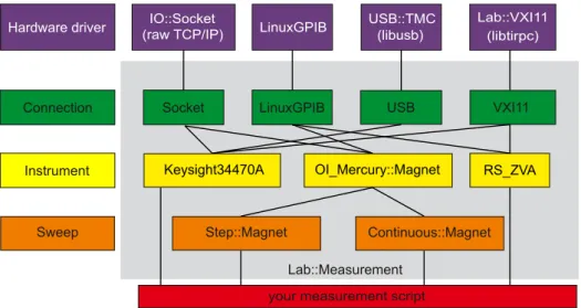
Lab::Measurement is implemented as an object-oriented layer structure of Perl modules, as displayed schematically in

The figure does not show the full set of provided modules, but demonstrates a small selection of hardware.

The uppermost layer depicted in the figure, corresponding to the

Lab::Measurement Perl module distribution. Several Perl binding modules such as Lab::VISA (comparable to the Python PyVISA module [15]), Lab::VXI11 , Lab::Zhinst , and USB::TMC are separately pro- vided by the Lab::Measurement authors via the Comprehensive Perl Archive Network (CPAN), as bindings to third-party libraries.

Conversely, e.g., the LinuxGPIB package [16] provides a Perl inter- face to its library and Linux kernel modules on its own.

The

provides a unified API to these hardware drivers, making it possible to address devices, send commands, and receive responses. It handles access to many common automation protocols, such as GPIB, USB-TMC, VXI-11, raw TCP Sockets, or for example the Zurich Instruments LabOne API.

An overview of the currently supported connection types is given in

The

represents connected test and measurement devices. The generic instrument class Lab::Moose::Instrument only provides means to send com- mands and receive responses; derived classes encapsulate the model-specific command sets. On this level, direct device program- ming can take place.

the Perl ecosystem. This means that it can be used and distributed according to the terms of either the GNU General Public License (version 1 or any later version) or the Artistic License; the choice of license is up to the user.

package Lab::Moose::Instrument::SR830; use Moose;

use Lab::Moose::Instrument qw/validated_getter validated_setter/;

use Lab::Moose::Instrument::Cache; extends ’Lab :: Moose :: Instrument ’;

with qw(

Lab::Moose::Instrument::Common );

# the initialization sub BUILD {

my $self = shift;

$self->clear(); $self->cls();

}

# reference signal frequency : declare cache cache frq => ( getter => ’ get_frq ’ );

# reference signal : get frequency sub get_frq {

my ( $self, %args ) = validated_getter( \@_ );

return $self->cached_frq(

$self->query( command => ’ FREQ ? ’, %args ) );

}

# reference signal : set frequency sub set_frq {

my ( $self, $value, %args )= validated_setter(

\@_, value => { isa => ’Num ’ } );

$self->write(

command => " FREQ $value ", %args );

$self->cached_frq($value);

}

# [...]

# measured value , get r and phi in one call sub get_rphi {

my ( $self, %args ) = validated_getter( \@_ );

my $retval = $self->query(

command => " SNAP ?3 ,4 ", %args );

my ( $r, $phi ) = split( ’,’, $retval );

chomp $phi;

return { r => $r, phi => $phi };

}

# [...]

Listing 1: Commented excerpt from the driver module for the Stan- ford Research SR830 lock-in amplifier; shown are the header and initialization, the functions for getting and setting the reference voltage frequency, and a function for reading out radius and phase of the measured signal.

The

finally provides abstraction of sweeping in- strument parameters and performing multi-dimensional measure- ments, with live plotting and data logging. This facilitates the creation of complex measurement tasks for non-programmers without creation of loops or conditional control flow statements.

3. Extending and programming the instrument layer 3.1. Minimal example of an instrument driver

Listing

shows a commented excerpt of an instrument driver module, based on the Stanford Research SR830 lock-in amplifier module distributed with Lab::Measurement .

Low level functionality in drivers is frequently implemented via Moose roles. These are an implementation of the concept of traits, which enable horizontal code reuse more efficiently than single inheritance, multiple inheritance, or mixins [13,17].

In our case, roles are used to share functions between different

instrument drivers. This significantly eases implementation of new

drivers compared to other open-source measurement frameworks,

e.g., [11,12]. The minimal driver of Listing

only consumes a single

role, Lab::Moose::Instrument::Common , providing, e.g., the

Fig. 1. Schematic of the internal structure ofLab::Measurement. The gray frame indicates modules that are part of theLab::MeasurementPerl distribution. For this example, as instrument hardware a Keysight 34470A digital multimeter, an Oxford Instruments Mercury iPS superconducting magnet controller, and a Rohde & Schwarz ZVA vector network analyzer are chosen.

Table 1

Available protocols and corresponding connection types. National Instruments (NI) VISA is only supported by NI on few Linux distributions and faces severe functional restrictions there due to the requirement of loading proprietary Linux kernel modules. In particular, USB GPIB adaptors are not supported by NI VISA on Linux.

Protocol Connection name Operating system support Description

Linux MS Windows

Multiple VISA (X) X National Instruments VISA architecture device access

GPIB LinuxGPIB X – IEEE 488 / GPIB adaptors supported by the LinuxGPIB project

VISA::GPIB (X) X IEEE 488 / GPIB frontend for VISA

IP, TCP Socket X X IP network sockets, mostly used for TCP connections

VXI-11 VXI11 X – VXI-11 protocol via SunRPC or libtirpc

VISA::VXI11 X X VXI-11 frontend for VISA

USB T&M USB X X USB Test & Measurement class device driver using libusb

VISA::USB (X) X USB Test & Measurement frontend for VISA

ZI LabOne Zhinst X X Zurich Instruments LabOne API

basic IEEE 488.2 standard commands. A more complex example demonstrating the usage of roles follows in Section

The code in the BUILD method is executed after instrument construction. Here we clear the device input and output buffers and any status or error flags. Otherwise we take care that driver initialization does not change any further device state; this is to ensure that, e.g., output voltages do not fluctuate on script start, or that manually applied configuration settings are kept unless explicitly overridden in the script.

The following code handles reading and setting the frequency of the ac voltage generated at the lock-in reference output. Hard- ware access is often slow, in particular regarding query operations, which is why we declare a cache for the frequency using function- ality from Lab::Moose::Instrument::Cache . The cache keeps track of frequency values written to the instrument, for fast later access. This assumes that device access is exclusive to the running script and no modifications on, e.g., a hardware front panel are taking place.

get_frq is provided to obtain the ac frequency of the refer- ence signal generated by the lock-in amplifier. It can be called with a hash of options as argument, which is validated by val- idated_getter and passed to the instrument query function.

The queried value of the frequency is cached and returned to the caller. set_frq sets the reference output ac frequency of the lock- in amplifier. It is called with a hash, which must contain a key

named value that provides the frequency value. The frequency is set by writing the corresponding command to the instrument;

subsequently the cache is updated with the frequency value.

The last stored cache value of the frequency can be accessed by the user with the cached_frq method. If this method is called when the cache entry is still empty, the getter method declared with the cache keyword, get_frq , is called to populate the cache.

In effect, cached_frq should be used in high-level functions whenever possible, except for situations where a hardware query needs to be enforced (refreshing the cache) with get_frq .

As opposed to the reference frequency, the signal amplitude and phase are not device parameters but measured values and thus cannot be set; the get_rphi function performs no caching.

It returns a reference to a hash with keys r and phi . In general, a design choice of Lab::Measurement is that functions always return a scalar variable; either directly a scalar value as, e.g., a frequency or a measured current, or a reference to a more complex Perl object.

The full SR830 driver contains several additional but simi-

larly implemented functions. This includes controlling reference

ac voltage amplitude, time constant, filter settings, input config-

uration, and sensitivity as well as reading out the signal as

,

,

, ϕ ^{). The}

functions are documented in POD syntax; the documentation can,

e.g., be read locally using perldoc or online on CPAN.

package Lab::Moose::Instrument::RS_FSV;

use 5.010;

use PDL::Core qw/pdl cat/;

use Moose;

use Moose::Util::TypeConstraints; use MooseX::Params::Validate;

use Lab::Moose::Instrument qw/timeout_param precision_param/;

use Carp;

use namespace::autoclean;

extends ’Lab :: Moose :: Instrument ’;

# ... and consumes the roles ...

with qw(

Lab::Moose::Instrument::Common Lab::Moose::Instrument::SCPI::Format

Lab::Moose::Instrument::SCPI::Sense::Bandwidth Lab::Moose::Instrument::SCPI::Sense::Frequency Lab::Moose::Instrument::SCPI::Sense::Sweep Lab::Moose::Instrument::SCPI::Initiate Lab::Moose::Instrument::SCPIBlock );

# initialization sub BUILD {

my $self = shift;

$self->clear(); $self->cls();

}

# get a spectrum trace sub get_spectrum {

my ($self, %args) = validated_hash(

\@_,

timeout_param() , precision_param() ,

trace => {isa => ’Int ’, default => 1} , );

# the FSV can store up to 6 traces my $trace = delete $args{trace};

if ($trace < 1 || $trace > 6) { croak " trace has to be in (1..6) "; }

# get frequency list ( from SCPI :: Sense :: Freq ) my $freq_array =

$self->sense_frequency_linear_array();

# make only one sweep ( from SCPI :: Initiate ) if ( $self->cached_initiate_continuous() ) {

$self->initiate_continuous( value => 0 ); }

# single or double precision ? ( from SCPIBlock ) my $precision = delete $args{precision};

$self->set_data_format_precision( precision => $precision );

# how much data will we read ? my $num_points = @{$freq_array};

$args{read_length} = $self->block_length(

precision => $precision, num_points => $num_points );

# run sweep ( from SCPI :: Initiate )

$self->initiate_immediate();

# wait for completion ( from Common , IEEE488 .2)

$self->wai();

# request binary trace data my $binary = $self->binary_query(

command => " TRAC ? TRACE$trace ",

%args );

# convert to PDL object

my $points_ref = pdl $self->block_to_array(

binary => $binary, precision => $precision );

# return it with frequency column prepended return cat((pdl $freq_array), $points_ref);

}

__PACKAGE__->meta() - >make_immutable();

1;

Listing 2: Commented Rohde & Schwarz FSV series spectrum ana- lyzer driver module.

3.2. Example instrument driver based on SCPI roles

Listing

provides an example of a more complex instrument driver module, at the example of a Rohde & Schwarz (R&S) FSV series spectrum analyzer. The driver strongly relies on the role functionality of Moose. The roles included in the R&S FSV driver with the with qw(...); statement mostly model the SCPI sub- systems [14] which comprise the command syntax of the instru- ment.

The high-level get_spectrum method, central part of the driver module, initiates a frequency sweep, reads the resulting spectrum from the instrument, and returns the data as a 2D array to the user. In the following, we discuss at its example how the different code parts interact in this method.

The FSV spectrum analyzer can be configured to record and store up to 6 frequency sweeps (called traces); the trace parame- ter can be used to address one of these. The precision parameter selects between double and single floating point precision as de- fined in the SCPI standard. The variable $freq_array is initialized with an array of the frequency values addressed within a sweep;

then the device is configured to perform only one sweep (instead of continuous, repeated measurement).

After calculating the size of the resulting data block, the sweep is started by calling the initiate_immediate method, pro- vided by the Lab::Moose::Instrument::SCPI::Initiate role. Calling the wai method from Instrument::Common

(cor- responding to the IEEE 488.2 command of the same name) waits until the operation has finished. Using binary_query from the base Instrument class, the measured data is read out once the sweep has completed.

The block_to_array method provided by the Instru- ment::SCPIBlock role is used to convert the raw IEEE 488.2 binary block data into a Perl array. The array is then subse- quently converted into a PDL (Perl Data Language) object, com- bined with the frequency array, and returned to the caller of the get_spectrum method. The returned PDL object can then be used for further processing or can be written to a datafile.

3.3. Instrument layer usage

The instrument layer is the lowermost layer typically used in measurement scripts. All functions of an instrument driver can here directly be accessed, allowing fine-grained control and spe- cialized programming. At the same time, the connection abstrac- tion is present, allowing instrument control independent of the precise operating system of the control PC running Lab::Measu rement or the wiring.

Listing

shows a brief example how to read out a Stanford Research SR830 lock-in amplifier connected via LinuxGPIB, using the driver discussed above. It sets the amplitude and frequency of the lock-in reference output. The new values are queried and printed together with the amplitude and phase of the measured signal.

Note that, as a consequence of abovementioned coding con- vention, get_rphi returns a scalar, namely a hash

returned values are thus accessed as, e.g., $rphi->{r} and

$rphi->{phi} .

A complete example of a measurement script based on the Lab::Moose::Sweep interface is given in Listing

. It is intended for a magnetic resonance experiment, where, e.g., a ferromag- netic sample is mounted on a coplanar waveguide and microwave

4For convenience we subsequently shorten role names.

# !/ usr / bin / env perl

# Read out SR830 lock - in amplifier use 5.010;

use Lab::Moose;

my $lia = instrument(

type => ’ SR830 ’,

connection_type => ’ LinuxGPIB ’, connection_options => {pad => 13}

);

$lia->set_amplitude(value => 0.5);

$lia->set_frq(value => 1000);

my $amp = $lia->get_amplitude();

say " Reference output amplitude : $amp V";

my $frq = $lia->get_frq();

say " Reference frequency : $frq Hz ";

my $rphi = $lia->get_rphi();

say " Signal : amplitude r= $rphi - >{r} V";

say " phase phi = $rphi - >{ phi } degree ";

Listing 3: Accessing a Stanford Research SR830 lock-in amplifier connected via LinuxGPIB on the instrument class level: reference signal amplitude and frequency as well as signal amplitude and phase are read out and displayed.

transmission is measured as a function of applied magnetic field.

The magnetic field is controlled with an Oxford Instruments (OI) Mercury iPS magnet controller; a Rohde & Schwarz (R&S) ZVA vec- tor network analyzer (VNA) is used for generating the microwave signal and detecting the complex transmission parameter

(f ).

Part A of the listing defines and initializes the connected remote-controlled instruments in the same way as already demon- strated in Listing

ethernet at fixed IP addresses, with the OI Mercury accepting plain TCP connections, and the R&S ZVA using VXI-11 protocol.

In part B, the two instruments are connected to so-called sweeps. The magnet controller is connected to a continuous mag- net sweep, which is internally defined by a class Lab::Moose::

Sweep::Continuous::Magnet . Multiple parameters such as start/stop points and the sweep rate are provided to the sweep function. The VNA is connected to a stepwise sweep of the output frequency. This way, the complex transmission will be measured at few discrete microwave frequencies; the VNA is doing fast ‘‘point measurements’’, instead of internally performing a frequency sweep.

Part C of Listing

defines the data file to be written. Data is recorded in the native GnuPlot [18] format as ASCII lines of tab- separated numerical values, with blank line separators after each conclusion of the innermost loop. The data file in addition contains a comment section with information on its columns; comment lines in the data file start with the hash character # and are ignored during plotting and evaluation.

In addition, here also a set of plot parameters of the data (‘‘a plot’’) is defined, referencing the column names of the data file. The plot will be displayed during the measurement and refreshed after each completion of the innermost measurement loop. This func- tionality for foreground operation is purely optional, and imple- mented using GnuPlot calls. Future work shall address the creation of more complex graphical user interface components, see e.g. [11].

Part D defines the measurement subroutine, a callback that is executed for each point in the addressed output parameter space.

In this example it reads out the momentary value of the magnetic field and performs a VNA ‘‘point measurement’’. As already noted, here the VNA is configured to only measure at a single frequency;

other types of VNA measurements are also available. The returned

$pdl object contains the frequency, real and imaginary parts of the

transmission parameter, as well as amplitude and phase of

# !/ usr / bin / env perl use 5.010;

use Lab::Moose;

# --- A: Initialize the instruments --- my $ips = instrument(

type => ’ OI_Mercury :: Magnet ’,

connection_type => ’ Socket ’, connection_options => {

host => ’ 192.168.3.15 ’ },

);

my $vna = instrument(

type => ’ RS_ZVA ’,

connection_type => ’ VXI11 ’, connection_options => {

host => ’ 192.168.3.27 ’ },

);

# Set VNA ’s IF filter bandwidth ( Hz )

$vna->sense_bandwidth_resolution(value => 1);

# --- B: Define the sweeps --- my $field_sweep = sweep(

type => ’ Continuous :: Magnet ’, instrument => $ips,

from => 2, # Tesla

to => 0, # Tesla

rate => 0.01 , # Tesla / min start_rate => 1, # Tesla / min

# ( rate to approach

# start point ) interval => 0, # run slave sweep

# as often as possible );

# Measure complex transmission at 1 ,2 ,... ,10 GHz my $frq_sweep = sweep(

type => ’ Step :: Frequency ’, instrument => $vna,

from => 1e9,

to => 10e9,

step => 1e9

);

# --- C: Create a data file and live plot --- my $datafile = sweep_datafile(

columns => [qw/B f Re Im r phi/]

);

# Add live plot of transmission amplitude

$datafile->add_plot(x => ’B ’, y => ’r ’);

# --- D: Measurement instructions --- my $meas = sub {

my $sweep = shift;

say " frequency f: ", $sweep->get_value();

my $field = $ips->get_field();

my $pdl = $vna->sparam_sweep(timeout => 10);

$sweep->log_block(

prefix => {field => $field}, block => $pdl

);

};

# --- E: Connect everything and go ---

$field_sweep->start(

slave => $frq_sweep, datafile => $datafile, measurement => $meas,

folder => ’ Magnetic_Resonance ’, );

Listing 4: Example measurement script based on the sweep layer.

An Oxford Instruments Mercury power supply is performing a continuous magnetic field sweep; in an inner loop, complex sig- nal transmission is measured by a Rohde & Schwarz ZVA vector network analyzer at several discrete frequency values. Data is recorded in Gnuplot format and plotted in real time.

the

parameter. This data is then logged with the log_block

command, inserting the momentary magnetic field as additional

column in front. The start method in part E finally starts the

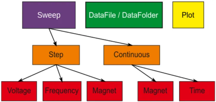
Fig. 2.Structural overview of the sweep and data logging classes.

--- id: 0

method: Clear ---

command: ’* CLS ’ id: 1

method: Write ---

command: ’* RST ’ id: 2

method: Write timeout: 10 ---

command: SNAP?1 ,2 id: 3

method: Query retval: " 0 ,0\ n"

timeout: 3

Listing 5: Example YAML log file for mock connection testing of the SR830 lock-in amplifier driver.

measurement via the outer (magnet) sweep and provides the glue connecting sweeps, data file, and measurement subroutine.

The overall design of the Lab::Measurement code is intended to provide a flexible high-level interface, while requiring only a minimum of programming knowledge for typical measurement tasks. Given their structure, the measurement scripts might even be pregenerated by a graphical user interface, while still allowing a maximum of internal tuning and adaption for the expert.

shows an overview of the classes is the sweep layer and the data logging framework. Data files and live plots are implemented as separate classes, which can also be used independently of the sweep functionality.

5. Quality control

Lab::Measurement is provided with a set of unit tests that can be run upon installation. The unit tests are integrated with the Github development repository via Travis [19] (for testing on Linux, under a wide range of Perl 5 versions) and Appveyor [20] (on Microsoft Windows) and run immediately on addition of new code commits. The current test status of the master branch is displayed on the Lab::Measurement homepage. In addition, release test reports on a wide range of software combinations, submitted by volunteers, are available via the CPANtesters website [21].

5.1. Testing with mock connection objects

Comprehensive testing of a large part of the provided func- tionality is impossible without having the corresponding hardware connected. To extend testing as far as possible, our testing routines simulate instrument responses using mock connection objects as described below.

A mock test consists of an ordinary measurement script which interfaces with one or more instruments. To select between logging

and mock operation, additional command line processing code is provided in the MockTest package, which is provided with the tests. The test script is first run connected to a real instrument.

Logging of the communication is provided by the instrument layer read , write , and query methods, independent of the specific instrument driver module. Each call to these methods is recorded with its arguments and the resulting return values into a human readable YAML text file, which is then stored alongside with the test script. An example log file for the SR830 lock-in amplifier is shown in Listing

.

Running a test without the connected instrument will use the Mock connection, which takes such a YAML log file as input.

Method calls on the mock connection will be compared with the recorded method calls; deviations from the log will lead to a test failure, allowing to ascertain the impact of committed code on the device communication. In case the test script provides the correct commands, the respective instrument responses are provided from the log file. This framework allows the creation of unit tests with considerably more coverage compared to those distributed in al- ternative open-source solutions [11,12].

6. Historical interface

Over the past years, Lab::Measurement has undergone sev- eral large scale revisions. Development was started in 2006, ini- tially only as a solution for addressing devices via the National Instruments (NI) VISA libraries [22,23] for Linux or MS Windows.

The code was later extended and refactored into a layer model, providing the abstractions for connections to instruments and instrument model specific features. The initial high-level interface focused only on logging and plotting, without providing any loop functionalities. Its successor, Lab::XPRESS , was added in 2012 and is with its documentation still present in the distribution for ongoing support of measurement scripts. The intent is to remove this deprecated code when all parts have been fully ported to Moose and Lab::Measurement 4 is released.

The historical stack uses an additional bus layer, in analogy to a GPIB adaptor carrying connections to several instruments.

All components are implemented using minimal object-oriented Perl. In the high-level interface, Lab::XPRESS , sweep classes, data logging and plotting are tightly integrated. A main objective of the Moose-based sweep classes was to modularize and simplify this part of the software, in order to allow easier integration of new features.

Aspects that still require porting to the new high-end Moose code include predefined command line switch handling for mea- surement scripts and customized handling of keyboard interrupts.

7. Requirements and licensing

Lab::Measurement is written in pure Perl and designed to run on any version since Perl 5.14. Given the extensive use of Moose and its object-oriented programming features, a range of Perl module dependencies is required. These, including minimum versions where applicable, are declared in the distribution meta- data META.json file included in the package and can be installed automatically by cpan or any Perl package manager.

The package is tested regularly and supported on both Linux

and Microsoft Windows, however, given availability of hardware

back-ends, should also work on other operating systems. Hardware

back-ends may require further dependencies, as, e.g., in the case

of Lab::VISA the National Instruments VISA driver stack, or in

the case of USB::TMC the libusb system library. Further details on these requirements can be found in the documentation of the back-end modules on CPAN.

Given that any plotting or graphical interface is optional and that the CPU and memory footprint of running Perl scripts is very low compared to commercial instrument control solutions [1,2], Lab::Measurement also lends itself for background control operation, logging, and headless server operation. The open source nature of its dependencies particularly on Linux allows the use ar- bitrary Linux systems, in particular including, e.g., ARM or AArch64 based embedded architectures.

As many other Perl module distributions, Lab::Measurement is released under the same license as Perl itself, meaning dual- licensed either under the Artistic License or the GNU General Public License, version 1 or any later version published by the Free Soft- ware Foundation. With this it is free and open source software, and can be downloaded from the Comprehensive Perl Archive Network (CPAN).

8. Summary

Lab::Measurement is a measurement framework designed for high portability and extensibility. The framework is in ac- tive use and was applied successfully in many condensed matter physics experiments. Its implementation consists of an object ori- ented layer structure. The connection layer provides backends for common instrumentation protocols on both Linux and Mi- crosoft Windows. The instrument layer, which represents con- nected equipment, uses modern object oriented programming techniques for code reuse. A high-level interface, suitable for users without previous Perl experience, allows fast creation of complex measurement tasks involving continuous or dis- crete sweeps of control parameters as, e.g., voltages, temper- ature, or magnetic field. By using mock connection objects, unit tests can be run without connected instruments. This al- lows safe refactoring and facilitates the future evolution of the framework.

Acknowledgments

We would like to thank E. E. Mikhailov for his helpful comments and considerable recent code contributions, and K. Fredric for in- sightful discussions. The authors thank the Deutsche Forschungs- gemeinschaft for financial support via SFB 689, GRK 1570, and Emmy Noether grant Hu 1808/1.

References

[1] National Instruments LabVIEW, URLhttp://www.ni.com/en-us/shop/labview.

html.

[2] MathWorks MATLAB & Simulink, URLhttps://www.mathworks.com/products /matlab.html.

[3] D. Schröer, A.D. Greentree, L. Gaudreau, K. Eberl, L.C.L. Hollenberg, J.P.

Kotthaus, S. Ludwig, Phys. Rev. B 76 (2007) 075306.http://dx.doi.org/10.1103/

PhysRevB.76.075306.

[4] D. Taubert, G.J. Schinner, H.P. Tranitz, W. Wegscheider, C. Tomaras, S. Kehrein, S. Ludwig, Phys. Rev. B 82 (2010) 161416.http://dx.doi.org/10.1103/PhysRevB.

82.161416.

[5] G. Granger, D. Taubert, C.E. Young, L. Gaudreau, A. Kam, S.A. Studenikin, P.

Zawadzki, D. Harbusch, D. Schuh, W. Wegscheider, Z.R. Wasilewski, A.A. Clerk, S. Ludwig, A.S. Sachrajda, Nat. Phys. 8 (7) (2012) 522–527.http://dx.doi.org/

10.1038/nphys2326.

[6] M. Gaass, A.K. Hüttel, K. Kang, I. Weymann, J. von Delft, C. Strunk, Phys. Rev.

Lett. 107 (2011) 176808.http://dx.doi.org/10.1103/PhysRevLett.107.176808.

[7] A. Dirnaichner, M. del Valle, K.J.G. Götz, F.J. Schupp, N. Paradiso, M. Grifoni, C.

Strunk, A.K. Hüttel, Phys. Rev. Lett. 117 (2016) 166804.http://dx.doi.org/10.

1103/PhysRevLett.117.166804.

[8] K.J.G. Götz, D.R. Schmid, F.J. Schupp, P.L. Stiller, C. Strunk, A.K. Hüttel, Phys. Rev.

Lett. 120 (2018) 246802.http://dx.doi.org/10.1103/PhysRevLett.120.246802.

[9] K.J.G. Götz, S. Blien, P.L. Stiller, O. Vavra, T. Mayer, T. Huber, T.N.G. Meier, M. Kronseder, C. Strunk, A.K. Hüttel, Nanotechnology 27 (13) (2016) 135202.

http://dx.doi.org/10.1088/0957-4484/27/13/135202.

[10] H. Maier, J. Ziegler, R. Fischer, D. Kozlov, Z.D. Kvon, N. Mikhailov, S.A. Dvoretsky, D. Weiss, Nature Commun. 8 (1) (2017) 2023. http://dx.doi.org/10.1038/

s41467-017-01684-0.

[11] PyMeasure scientific package, URLhttps://pymeasure.readthedocs.io/.

[12] QCoDeS —Python-based data acquisition framework developed by the Copen- hagen / Delft / Sydney / Microsoft quantum computing consortium, URLhttp:

//qcodes.github.io/Qcodes/.

[13] S. Ducasse, O. Nierstrasz, N. Schärli, R. Wuyts, A.P. Black, ACM Trans. Pro- gram. Lang. Syst. 28 (2) (2006) 331–388.http://dx.doi.org/10.1145/1119479.

1119483.

[14] SCPI Consortium, Standard commands for programmable instrumentation (SCPI), URLhttp://www.ivifoundation.org/docs/scpi-99.pdf.

[15] PyVISA —Python package for support of VISA, URLhttps://pyvisa.readthedocs.

io/en/stable/.

[16] F.M. Hess, D. Penkler, et al. LinuxGPIB. Support package for GPIB (IEEE 488) hardware, containing kernel driver modules and a C user-space library with language bindings, URLhttp://linux-gpib.sourceforge.net/.

[17] T. Inkster, Horizontal Reuse: An Alternative to Inheritance, URLhttp://radar.

oreilly.com/2014/01/horizontal-reuse-an-alternative-to-inheritance.html.

[18] T. Williams, C. Kelley, E.A. Merritt, et al. gnuplot — An interactive plotting program, URLhttp://www.gnuplot.info/.

[19] Travis CI continuous integration system, URLhttp://travis-ci.org/.

[20] Appveyor Continuous Integration solution for Windows, URLhttps://www.

appveyor.com/.

[21] cpantesters.org test reports for Lab::Measurement, URLhttp://matrix.cpantes ters.org/?dist=Lab-Measurement.

[22] National Instruments Virtual Instrument Software Architecture (VISA), URL https://www.ni.com/visa/.

[23] VISA Specifications, URLhttp://www.ivifoundation.org/specifications/default.

aspx.