Unmanned aerial vehicles (UAVs) for multi-temporal crop surface modelling
-
A new method for plant height and biomass estimation based on RGB-imaging
I n a u g u r a l - D i s s e r t a t i o n zur
Erlangung des Doktorgrades
der Mathematisch-Naturwissenschaftlichen Fakultät der Universität zu Köln
vorgelegt von Juliane Viktoria Bendig
aus Neuss Köln, 2015
Berichterstatter: Prof. Dr. Georg Bareth Prof. Dr. Karl Schneider Tag der mündlichen Prüfung: 12.01.2015
Abstract
Data collection with unmanned aerial vehicles (UAVs) fills a gap on the observational scale in re- mote sensing by delivering high spatial and temporal resolution data that is required in crop growth monitoring. The latter is part of precision agriculture that facilitates detection and quan- tification of within-field variability to support agricultural management decisions such as effective fertilizer application. Biophysical parameters such as plant height and biomass are monitored to describe crop growth and serve as an indicator for the final crop yield. Multi-temporal crop surface models (CSMs) provide spatial information on plant height and plant growth.
This study aims to examine whether (1) UAV-based CSMs are suitable for plant height modelling, (2) the derived plant height can be used for biomass estimation, and (3) the combination of plant height and vegetation indices has an added value for biomass estimation.
To achieve these objectives, UAV-flight campaigns were carried out with a red-green-blue (RGB) camera over controlled field experiments on three study sites, two for summer barley in Western Germany and one for rice in Northeast China. High-resolution, multi-temporal CSMs were derived from the images by using computer vision software following the structure from motion (SfM) approach. The results show that plant height and plant growth can be accurately modelled with UAV-based CSMs from RGB imaging. To maximise the CSMs’ quality, accurate flight planning and well-considered data collection is necessary. Furthermore, biomass is successfully estimated from the derived plant height, with the restriction that results are based on a single-year dataset and thus require further validation. Nevertheless, plant height shows robust estimates in comparison with various vegetation indices. As for biomass estimation in early growth stages additional po- tential is found in exploiting visible band vegetation indices from UAV-based red-green-blue (RGB) imaging. However, the results are limited due to the use of uncalibrated images. Combining visible band vegetation indices and plant height does not significantly improve the performance of the biomass models.
This study demonstrates that UAV-based RGB imaging delivers valuable data for productive crop monitoring. The demonstrated results for plant height and biomass estimation open new possi- bilities in precision agriculture by capturing in-field variability.
Zusammenfassung
Die Datenerfassung mit Unmanned Aerial Vehicles (UAVs) füllt eine Lücke auf der Beobachtungs- skala in der Fernerkundung durch die Bereitstellung von Daten mit hoher räumlicher und zeitlicher Auflösung, die für die Überwachung von Pflanzenwachstum erforderlich sind. Letzteres ist Teil der Präzisionslandwirtschaft, welche die Erfassung und Quantifizierung von Variabilität innerhalb von Getreidebeständen ermöglicht und so Entscheidungen des landwirtschaftlichen Managements unterstützt wie zum Beispiel bei effizienter Düngung. Die Überwachung biophysikalischer Para- meter wie Pflanzenhöhe und Biomasse dient der Erfassung des Pflanzenwachstums und liefert Indikatoren für den Ertrag. Multitemporale Oberflächenmodelle von Getreidebeständen (crop surface models - CSMs) liefern räumliche Informationen über die Pflanzenhöhe und das Pflanzen- wachstum.
Ziel dieser Studie ist es zu prüfen, ob (1) UAV-basierte CSMs sich zur Modellierung der Pflanzen- höhe eignen, (2) die abgeleitete Pflanzenhöhe für Biomasseschätzungen verwendet werden kann, und (3) die Kombination von Pflanzenhöhe und Vegetationsindizes einen Mehrwert für Biomasse- schätzung hat.
Um diese Ziele zu erreichen, wurden UAV-Flugkampagnen mit einer Rot-Grün-Blau (RGB)-Kamera in kontrollierten Feldversuchen in drei Untersuchungsgebieten durchgeführt, zwei für Sommer- gerste in Westdeutschland und eine für Reis im Nordosten Chinas. Aus den Bildern wurden hoch aufgelöste, multitemporale CSMs mit Hilfe von Computer-Vision-Software nach dem Structure from Motion (SFM) Ansatz abgeleitet. Die Ergebnisse zeigen, dass es genaue Modellierungen der Pflanzenhöhe und des Pflanzenwachstums mit UAV-basierten CSMs aus RGB Aufnahmen möglich sind. Um die Qualität der CSMs zu maximieren, sind eine genaue Flugplanung und wohlüberlegte Datenerfassung notwendig. Weiterhin lässt sich Biomasse erfolgreich mit der abgeleiteten Pflan- zenhöhe schätzen, mit der Einschränkung, dass die Ergebnisse aus einem einjährigen Datensatz erzeugt wurden und folglich eine weitere Verifizierung erfordern. Dennoch, zeigen die Schätzun- gen mittels Pflanzenhöhe robuste Ergebnisse im Vergleich mit verschiedenen Vegetationsindizes.
Für die Biomasseschätzung in frühen Wachstumsstadien, zeigt sich zusätzliches Potential für die Biomasseschätzung mittels Vegetationsindizes im Bereich des sichtbaren Lichts, die aus UAV-ba- sierten Rot-Grün-Blau (RGB) Aufnahmen abgeleitet wurden. Eine Beschränkung der Ergebnisse ergibt sich aus der Verwendung von unkalibrierten Bildern. Die Kombination von Vegetationsindi- zes im Bereich des sichtbaren Lichts und der Pflanzenhöhe führte nicht zu einer signifikanten Ver- besserung in der Vorhersagequalität der Biomasse-Modelle.
Diese Studie zeigt, dass RGB-Aufnahmen auf der Basis von UAVs wertvolle Daten für die produk- tive Überwachung von Pflanzenwachstum liefern. Die gezeigten Ergebnisse für die Pflanzenhöhe und Biomasseschätzung eröffnen neue Möglichkeiten in der Präzisionslandwirtschaft durch die Erfassung von Variabilität innerhalb von Getreidebeständen.
Acknowledgements
This dissertation and my entire time at the University of Cologne was a journey for me, a journey on which I met people who determined my itinerary. I would like to thank my supervisor Prof. Dr.
Georg Bareth who introduced me to the world of remote sensing, who provided me the best ed- ucational opportunities in various places around the world and who often infected me with his enthusiasm. I would like to thank Dr. Andreas Bolten, Max Willkomm, Helge Aasen and all my other colleagues for support on the “dull, dirty and [thankfully rarely, J.B.] dangerous [UAV, J.B.]
missions” (VAN BLYENBURGH, 1999). Furthermore, I thank Dr. Andreas Bolten for teaching me so much technical know-how during building our small UAV fleet and for his editorial support. I thank Dr. Martin Gnyp for his highly constructive food for thought during the preparation of this disser- tation. I thank my mother for her patient proof reading and the rest of my family and friends for their valuable moral support.
For the study site in Rheinbach I acknowledge the funding of the CROP.SENSe.net project in the context of Ziel 2-Programms NRW 2007-2013 “Regionale Wettbewerbsfähigkeit und Bes- chäftigung (EFRE)” by the Ministry for Innovation, Science and Research (MIWF) of the state North Rhine Westphalia (NRW) and European Union Funds for regional development (EFRE) (005-1103- 0018).
For the study site in Jiansanjiang I acknowledge the The International Center for Agro-Informatics and Sustainable Development (ICASD).
Cologne was an excellent base camp for this journey. Let's see how it continues…
Table of Contents
ABSTRACT ... I ZUSAMMENFASSUNG ... II ACKNOWLEDGEMENTS ... IV TABLE OF CONTENTS ... V
1 INTRODUCTION ... 1
1.1 PREFACE ... 1
1.2 RESEARCH PROBLEM AND AIMS ... 3
1.3 OUTLINE ... 6
2 BASICS AND METHODS ... 8
2.1 BIOMASS ESTIMATION FROM REMOTE SENSING DATA ... 8
2.2 PLANT HEIGHT,PLANT GROWTH AND CROP SURFACE MODELS ... 8
2.3 UAVREMOTE SENSING ... 10
2.3.1 UAVs ... 10
2.3.2 DSMs/DEMs from UAV-based RGB Imaging ... 12
2.4 MEASURING SPECTRAL PROPERTIES OF PLANTS ... 15
2.4.1 Reflectance ... 15
2.4.2 Vegetation Indices ... 17
2.5 AGRONOMY OF BARLEY AND RICE ... 19
2.5.1 Barley ... 19
2.5.2 Rice ... 20
2.6 STUDY SITES ... 21
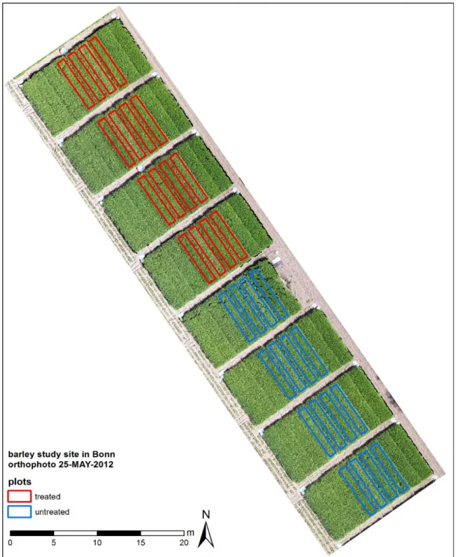
2.6.1 Barley – Bonn (2012) ... 21
2.6.2 Barley – Rheinbach (2013) ... 23
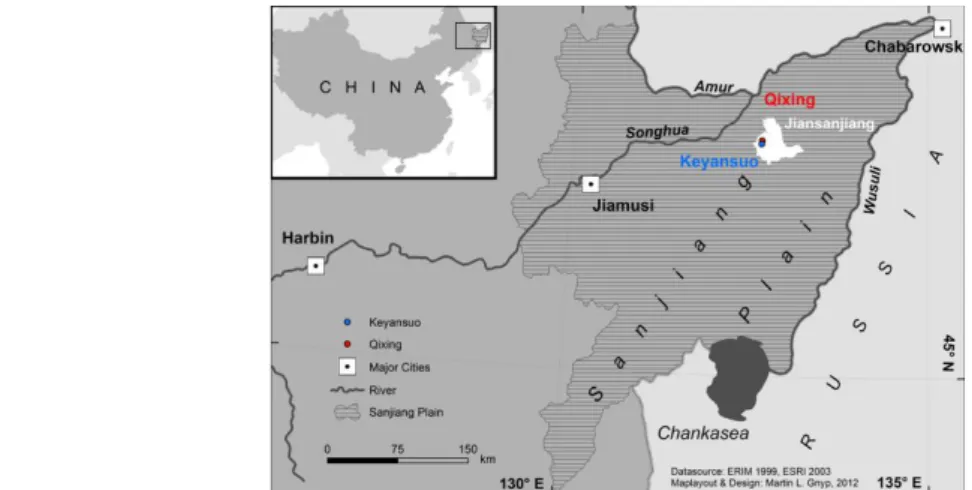
2.6.3 Rice – Jiansanjiang, China (2012) ... 24
3 HOCH AUFLÖSENDE CROP SURFACE MODELS (CSMS) AUF DER BASIS VON STEREOBILDERN AUS UAV-BEFLIEGUNGEN ZUR ÜBERWACHUNG VON REISWACHSTUM IN NORDOSTCHINA ... 26
3.1 INTRODUCTION ... 28
3.2 DATA AQUISITION ... 29
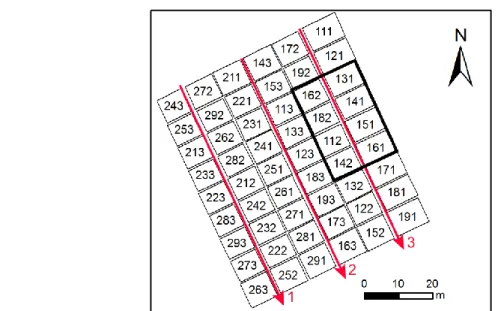
3.2.1 Study Area and Dataset ... 29
3.2.2 Platform ... 30
3.2.3 Sensor ... 31
3.2.4 Measurement ... 31
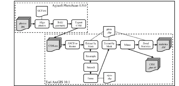
3.2.5 Data Processing ... 32
3.3 RESULTS ... 35
3.3.1 Statistics... 35
3.3.2 Crop Surface Models ... 36
3.3.3 Crop Growth ... 37
3.4 DISCUSSION ... 38
3.5 CONCLUSION ... 40
3.6 OUTLOOK ... 40
4 UAV-BASED IMAGING FOR MULTI-TEMPORAL, VERY HIGH RESOLUTION CROP SURFACE
MODELS TO MONITOR CROP GROWTH VARIABILITY ... 44
4.1 INTRODUCTION ... 45
4.2 DATA ACQUISITION ... 46
4.2.1 Study Area and Dataset ... 46
4.2.2 Platform ... 48
4.2.3 Sensor ... 48
4.2.4 Data Acquisition ... 49
4.2.5 Data Processing ... 49
4.3 RESULTS ... 51
4.3.1 Statistics... 51
4.3.2 Crop Surface Models ... 52
4.3.3 Plant Height Development... 53
4.3.4 Accuracy Assessment ... 54
4.4 DISCUSSION AND CONCLUSION ... 55
4.5 OUTLOOK ... 58
5 ESTIMATING BIOMASS OF BARLEY USING CROP SURFACE MODELS (CSMS) DERIVED FROM UAV-BASED RGB IMAGING ... 61
5.1 INTRODUCTION ... 62
5.2 MATERIALS AND METHODS ... 63
5.2.1 Test Site: Campus Klein-Altendorf, 2013 ... 63
5.2.2 Biomass Sampling ... 64
5.2.3 Platform ... 65
5.2.4 Sensor ... 66
5.2.5 Generating CSMs ... 66
5.2.6 Statistical Analyses ... 67
5.3 RESULTS ... 68
5.3.1 Plant Height and Biomass Samples ... 68
5.3.2 Biomass Modelling ... 70
5.4 DISCUSSION ... 73
5.5 CONCLUSIONS AND OUTLOOK ... 76
6 COMBINING UAV-BASED CROP SURFACE MODELS, VISIBLE AND NEAR INFRARED VEGETATION INDICES FOR BIOMASS MONITORING IN BARLEY ... 83
6.1 INTRODUCTION ... 84
6.2 MATERIALS AND METHODS ... 85
6.2.1 Test Site ... 85
6.2.2 Biomass Sampling and BBCH Measurements ... 86
6.2.3 UAV-based Data Collection ... 86
6.2.4 Field Spectroradiometer Measurements ... 87
6.2.5 Plant Height generation from CSM ... 88
6.2.6 Vegetation Indices ... 88
6.2.7 Statistical Analyses ... 90
6.3 RESULTS ... 91
6.3.1 Plant Height and Biomass Samples ... 91
6.3.2 Biomass Modelling ... 91
6.4 DISCUSSION ... 96
6.5 CONCLUSIONS AND OUTLOOK ... 97
7 LOW-WEIGHT AND UAV-BASED HYPERSPECTRAL FULL-FRAME CAMERAS FOR MONITORING CROPS: SPECTRAL COMPARISON WITH PORTABLE SPECTRORADIOMETER MEASUREMENTS ... 103
7.1 INTRODUCTION ... 104
7.2 STUDY AREA,UAV, AND SENSORS ... 105
7.3 SPECTRAL COMPARISONS ... 108
7.4 DISCUSSION AND CONCLUSIONS ... 114
8 DISCUSSION ... 119
8.1 ACCURACY OF CROP SURFACE MODELS FROM UAV-BASED RGBIMAGING ... 119
8.2 UNCERTAINTIES IN PLANT HEIGHT MODELLING ... 122
8.3 POTENTIALS OF BIOMASS ESTIMATION FROM CROP SURFACE MODELS ... 123
8.4 COMBINING VEGETATION INDICES AND CROP SURFACE MODELS FOR BIOMASS ESTIMATION ... 125
8.5 ADDITIONAL APPLICATIONS OF UAV-BASED IMAGING AND CROP SURFACE MODELS ... 127
8.6 LIMITS OF THE METHOD AND DATASET ... 131
9 CONCLUSIONS AND FUTURE CHALLENGES ... 133
REFERENCES*CHAPTERS 1,2,8,9 ... 135
LIST OF FIGURES AND TABLES ... 147
APPENDIX A: EIGENANTEIL ZU KAPITEL 3 ... 151
APPENDIX B: EIGENANTEIL ZU KAPITEL 4 ... 152
APPENDIX C: EIGENANTEIL ZU KAPITEL 5 ... 153
APPENDIX D: EIGENANTEIL ZU KAPITEL 6 ... 154
APPENDIX E: EIGENANTEIL ZU KAPITEL 7... 155
APPENDIX F: ERKLÄRUNG ... 156
APPENDIX G: CURRICULUM VITAE ... 157
1 Introduction
1.1 Preface
In recent times the world’s agricultural production system faces a number of challenges (OLIVER ET AL., 2013). Today’s agriculture and natural resources are pressured by population growth, increas- ing consumption of calorie- and meat-intensive diets and increasing use of cropland for non-food use like biofuel (FOLEY ET AL., 2011; FOOD AND AGRICULTURE ORGANIZATION OF THE UNITED NATIONS, 2013; MUELLER ET AL., 2012). Population growth is accompanied by a decrease in available land.
Furthermore, climate change will alter the reliability of critical components in crop production that causing production variability (ATZBERGER, 2013; SRINIVASAN AND SRINIVASAN, 2006). Crop pro- duction can be quantified by agronomic parameters such as crop yield, leaf area index (LAI) or chlorophyll content (HATFIELD ET AL., 2008). Parameters describing the crop status can be linked to climate modelling, for example when changing weather patterns cause production variability be- tween two growing seasons. Within fields, variability is a result of soil quality, drainage conditions, physiography, aspect, salinity and nutrient management (OLIVER ET AL., 2013). Additionally, varia- bility may be of spatial or temporal nature. Spatial variability occurs across certain areas, whereas temporal variability occurs at different measurement times (WHELAN AND TAYLOR, 2013). Particu- larly, soil variability is closely linked to crop growth and hence crop production (ADAMCHUK ET AL., 2010). On the field and sub-field scale both natural variability as well as historic and recent man- agement factors influence crop production. Humans have an impact on crop production variability through management decisions. Precision agriculture is a way of addressing production variability and optimising management decisions.
Precision agriculture accounts for production variability and uncertainties, optimises resource use and protects the environment (GEBBERS AND ADAMCHUK, 2010; MULLA, 2013). By definition, a com- plete precision agriculture system consists of four aspects: (1) field variability sensing and infor- mation extraction, (2) decision making, (3) precision field control, and (4) operation and result assessment (YAO ET AL., 2011). Precision agriculture adapts management practises within an agri- cultural field, according to variability in site conditions (SEELAN ET AL., 2003). Consequently, there is a need for methods for characterizing such variability. Within-field crop monitoring is needed to describe site conditions with a high spatial and temporal resolution (CAMPBELL AND WYNNE, 2011). In precision agriculture detailed in-field information is retrieved from using Global Position-
ing Systems (GPS), Geographical Information Systems (GIS) and Remote Sensing (RS) for agricul- tural decision making (SEELAN ET AL., 2003). This information is required within a short time window for agricultural management (HUNT JR. ET AL., 2013). RS provides such timely information for as- sessing within-field variability to adapt agricultural management purposes (ATZBERGER, 2013).
Once knowing the site conditions, fertilisers, herbicides and pesticides are only applied where and when they are needed (BONGIOVANNI AND LOWENBERG-DEBOER, 2004; NELLIS ET AL., 2009). Ultimately, profitability increases and environmental contamination minimizes (WHELAN AND TAYLOR, 2013).
As a result, RS techniques are commonly used for crop monitoring (ATZBERGER, 2013; CLEVERS AND
JONGSCHAAP, 2001).
Advances in computing, position-locating technologies and sensor development increased possi- bilities for using RS as an important data source of spatial and temporal information to adjust site- specific crop management (PINTER ET AL., 2003; SHANAHAN ET AL., 2001). RS refers to obtaining in- formation from an object or phenomenon without getting into physical contact with it (LILLESAND ET AL., 2008). In an agricultural context, RS includes non-destructive methods for crop monitoring opposed to destructive sampling and laboratory-based measurements (CAMPBELL AND WYNNE, 2011). Typically, RS records the surface reflectance in the visible or near-infrared parts of the elec- tromagnetic spectrum (YAO ET AL., 2011). Reflectance is linked to crop biophysical parameters such as biomass or leaf area index (LAI) that indicate the final crop yield (COHEN ET AL., 2003). RS data is acquired fast and in high spatial and temporal detail compared to time, cost and labour-intensive destructive sampling (ATZBERGER, 2013). Costs for RS data vary depending on the sensor and carrier platform (LILLESAND ET AL., 2008). RS methods are classified according to the sensor type as either passive or active and according to the carrier platform. Passive RS employs instruments that sense emitted energy like optical or thermal sensors opposed to active RS with sensors emitting their own energy like radar or LIDAR sensors (CAMPBELL AND WYNNE, 2011). Sensors are carried by space- borne, manned or unmanned airborne or ground-based platforms (proximate sensing) (MULLA, 2013). The platform determines the distance to the sensed object, resulting in a local, regional or global study scale. Common platforms for local scale studies include small aircraft and unmanned airborne platforms. The latter are referred to as unmanned aerial vehicles (UAVs), unmanned aer- ial systems (UAS) or remotely piloted aerial systems (RPAS) (COLOMINA AND MOLINA, 2014). UAV platforms are increasingly used in RS applications as demonstrated by COLOMINA AND MOLINA
(2014), HARDIN AND JENSEN (2011a) and LALIBERTE ET AL. (2011), who give examples of different plat- forms and applications.
1.2 Research Problem and Aims
Agricultural production is influenced by the following variabilities: yield variability, field variability, soil variability, crop variability, anomalous factor variability and management variability (OLIVER ET AL., 2013; ZHANG ET AL., 2002). Those variabilities result in differences in crop growth within agri- cultural fields that can be quantified by monitoring crop canopy variables throughout the growing season. Important variables in this context include leaf area index (LAI), biomass, and nitrogen status (HANSEN AND SCHJOERRING, 2003; SERRANO ET AL., 2000). Biomass and nutrient use efficiency are considered as the main influencing factors on final crop yield (RAUN AND JOHNSON, 1999). More- over, biomass has a strong relationship with nitrogen (JENSEN ET AL., 1990; VAN KEULEN ET AL., 1989).
Since nitrogen is an essential nutrient in crop production, it is often over-applied with negative impacts on yield and environment (HATFIELD ET AL., 2008). Knowledge on crop status and condition can be used to effectively improve nitrogen application by eliminating nutrient overuse (ATZBERGER, 2013; NELLIS ET AL., 2009). In this context, the nitrogen nutrition index (NNI) is a pow- erful tool for assessing crop nitrogen status (MISTELE AND SCHMIDHALTER, 2008). The NNI is defined as the ratio of measured and critical nitrogen content. Biomass and nitrogen concentration are input values for the N dilution curve from which the critical nitrogen content is determined (LE- MAIRE ET AL., 2008; LEMAIRE AND GASTAL, 1997). Therefore, biomass is of major importance in in crop growth monitoring. Studies by MORIONDO ET AL. (2007), REMBOLD ET AL. (2013), and MARCELIS ET AL. (1998) give examples for quantifying crop growth by measuring daily biomass gains. The accumu- lated biomass may be multiplied by a harvest index to simulate the final yield.
Data for monitoring crop growth is most valuable when captured with high spatial and temporal resolution to properly detect the variability within an agricultural field. The advantage of using unmanned aerial vehicles (UAVs) for crop growth monitoring is that UAVs fill a niche of observa- tional scale, resolution and height between manned aerial platforms and the ground (SWAIN AND
ZAMAN, 2012). Low distance from the sensed object enables collection of high resolution data and minimizes atmospheric effects in images. A mayor advantage over satellite imagery is the inde- pendence of clouds and revisit time and fast data acquisition with real time capability (BERNI ET AL., 2009a; EISENBEISS, 2009). Furthermore, high temporal resolution is given through high flexibil- ity in data acquisition (ABER ET AL., 2010; SHAHBAZI ET AL., 2014). Those characteristics make UAVs highly suitable for many agricultural applications (JENSEN ET AL., 2007; SWAIN AND ZAMAN, 2012).
Examples include spraying from unmanned helicopters that is most popular in Japan where more than 10% of paddy fields are sprayed by using this technique (NONAMI ET AL., 2010).
Generally, the growing interest in UAV systems produces a rapidly growing market with a pre- dicted growth from 5400.0 M€ market value in 2013 up to 6350.0 M€ by 2018 (MARKETSANDMAR- KETS, 2013). The number of available UAV systems multiplied by three from 2005 to the present (COLOMINA AND MOLINA, 2014) with a relevant increase in civil/commercial platforms (NONAMI ET AL., 2013). The advice of market researchers is: “Let them fly and they will create a new remote sensing market in your country” (MARKETSANDMARKETS, 2013). Trends in UAV technology include autonomous flights and swarm flights with multiple UAVs. Due to a rapid development in micro- controller processing speed and storage capacity the ability of UAVs to perform such complex tasks is increasing (NONAMI ET AL., 2013; VALAVANIS AND VACHTSEVANOS, 2014). Consequently, sensor development goes in the direction of lighter sensors with high performance. For example, light- weight full-frame hyperspectral cameras, airborne laser scanners and inertial measurement units (IMUs) became available for the use on small UAVs weighing 0.5 to 5 kg with 0.3 to 1.5 h endur- ance (BARETH ET AL., 2015; COLOMINA AND MOLINA, 2014; WALLACE ET AL., 2012). Those developments result in a strong demand for research on robust methodologies in the field of RS and crop moni- toring. However, more attention should be paid to development and evaluation of data processing techniques (SHAHBAZI ET AL., 2014). Data acquisition and data processing for many new sensors are at an experimental stage and improvement is needed to make it available to end users that might be the farmers.
Several authors demonstrate how UAVs in combination with light weight sensors are used for crop monitoring. Crop health is the most popular topic in this context (SHAHBAZI ET AL., 2014), demon- strated for example by HUANG ET AL.(2010) for cotton fields, NEBIKER ET AL.(2008) for vineyards, and CALDERÓN ET AL. (2014) for opium poppy. Further research investigates water stress for exam- ple in orchards and vineyards by using thermal and multispectral sensors (BALUJA ET AL., 2012;
BELLVERT ET AL., 2014; BERNI ET AL., 2009a). Existing UAV-based studies on crop growth monitoring include assessing biomass and nitrogen status (HUNT JR. ET AL., 2005), and deriving vegetation in- dices to relate them to LAI or nitrogen uptake (HUNT,JR. ET AL., 2010; LELONG, 2008; SWAIN AND
ZAMAN, 2012). In addition, plant height is an important parameter in crop growth monitoring.
Numerous methods for measuring plant height on the ground exist (for example BUSEMEYER ET AL., 2013; EHLERT ET AL., 2009), but fail to produce accurate and precise data at high spatial and tem- poral resolution (GRENZDÖRFFER AND ZACHARIAS, 2014). Additionally, those methods are not suitable for high growing crops like maize and sugarcane as well as irrigated crops like paddy rice. In those
cases, UAVs significantly simplify plant height measurements. EISENBEISS (2009)demonstrates dig- ital surface model (DSM) generation in a maize field. Further examples of plant height measure- ments from UAVs are given by HONKAVAARA ET AL. (2013) in wheat and barley, by GRENZDÖRFFER AND ZACHARIAS (2014) in wheat and GEIPEL ET AL. (2014) in maize. However, studies are missing where plant height is systematically monitored throughout the growing period based on UAV data.
This study utilizes remotely sensed crop surface models (CSMs) to produce high spatial and tem- poral resolution plant height data. CSMs are 3D models of the canopy surface derived from RS data (HOFFMEISTER ET AL., 2010). The concept is successfully applied on terrestrial laser scanning (TLS) data (HOFFMEISTER ET AL., 2010; TILLY ET AL., 2014). Transferring the CSM concept to UAV data is one key goal of this research.
A second goal is to model crop biomass based on plant height derived from UAV-based CSMs.
Today, it is common practice to derive biomass from plant height since crop yield is linked to crop growth and crop yield is directly linked to biomass (SERRANO ET AL., 2000). LATI ET AL. (2013b) esti- mated biomass from plant volume for single plants. PORDESIMO ET AL. (2004) found good relation- ships between stalk diameter and plant height for biomass estimation in corn stover. CATCHPOLE AND WHEELER (1992) give various examples for ground-based biomass estimation from plant height. Moreover, common tractor-based plant height measurement techniques aim at predicting biomass (BUSEMEYER ET AL., 2013; EHLERT ET AL., 2009). LUMME ET AL.(2008) and TILLY ET AL. (2014) estimate biomass using TLS. Following the argumentation that biomass can be estimated from plant height the hypothesis arises if biomass can estimated from UAV-based CSMs.
A third goal is to combine CSMs and vegetation indices. Vegetation indices that use reflectance in the near-infrared are a well-established method for biomass estimation (KUMAR ET AL., 2001; QI ET AL., 1994; ROUSE ET AL., 1974). PERRY AND ROBERTS (2008) investigate the relationship of visible band vegetation indices and biomass. UAV-based imagery enables calculation of visible band vegetation indices. It follows that biomass estimation should benefit from combining plant height and vege- tation indices. Both vegetation indices from ground-based hyperspectral measurements and UAV- data are suitable for that combination. In conclusion, key research questions are:
Are UAV-based CSMs suitable for plant height modelling?
Are UAV-based CSMs suitable for biomass estimation?
Does a combination of plant height and vegetation indices improve biomass estimation?
1.3 Outline
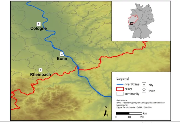
The introduction, chapter 1, is followed by a specification of the basic principles and methods used, chapter 2. First, ways the estimate biomass from remote sensing data are presented. Sec- ondly, methods for plant height and plant growth measurement are outlined and the principle of crop surface models (CSMs) is described. The next section introduces the method of UAV remote sensing, divided in a general UAV section and a description of 3D surface generation from red- green-blue (RGB) imaging. After that, methods for measuring spectral properties of plants are ex- plained with regard to the focus of this research. The term reflectance is introduced and vegeta- tion indices are presented as a method for expressing and comparing reflectance. Chapter 2 con- cludes with a brief introduction to the basic agronomy of barley and rice and a description of the study sites. The study sites are located in Bonn and Rheinbach (Germany) for summer barley and in Jiansanjiang (China) for rice. Chapters 3 to 7 comprise five research papers with the following content:
In chapter 3 (BENDIG ET AL., 2014b) the CSM generation process from RGB imaging is described for the rice study site in China. In this context, CSM generation process is adapted to the conditions of an irrigated rice field.
In chapter 4 (BENDIG ET AL., 2013) CSMs to monitor crop growth in summer barley are evaluated.
Detected crop growth variability is evaluated with ground-based in-field control surveys of plant height, indicating a strong relationship between CSM-derived plant height and in-field control sur- veys. Results are verified in an accuracy assessment.
In chapter 5 (BENDIG ET AL., 2014a) a biomass model is developed based on CSMs derived from UAV-based images. The CSMs are validated with in-field plant height ground measurements. For fresh and dry biomass estimation five linear regression models are tested in a cross validation. A strong correlation is found between plant height and fresh biomass, and plant height and dry bi- omass.
In chapter 6 (BENDIG ET AL., submitted) CSM-derived plant height and vegetation indices are eval- uated for biomass estimation. Vegetation indices are calculated from hyperspectral data and RGB imagery. Plant height shows the strongest relationship with dry biomass across all growth stages.
Visible band vegetation indices have potential for biomass estimation in early growth stages.
In chapter 7 (BARETH ET AL., 2015) two UAV-based hyperspectral full-frame cameras are compared with a field spectroradiometer. The images of the hyperspectral full-frame camera are consistent with the measurements from the field spectroradiometer.
The discussion, chapter 8, addresses the accuracy of CSMs from UAV-based RGB imaging and gen- eral uncertainties in plant height modelling. Further discussion points include both, potentials of biomass estimation from CSMs and combining vegetation indices and CSMs for biomass estima- tion. Subsequently, additional applications of CSMs are presented. At the end, the methods’ and dataset’s limits are outlined.
Chapter 9 concludes significant achievements of this research and summarises future research opportunities.
2 Basics and Methods
2.1 Biomass Estimation from Remote Sensing Data
The term biomass refers to the weight of living material, usually expressed as dry weight, in all or parts of an organism, population or community (KUMAR, 2006). It is commonly expressed as weight per unit area. Biomass accumulates through photosynthesis when solar radiation is converted into carbon dioxide (CO2) and water (H2O) (KUMAR ET AL., 2001; VARGAS ET AL., 2002). Plants grow through photosynthesis and develop plant organs above and below the ground. Grasses like bar- ley and rice develop underground root biomass and above ground biomass. The above ground biomass includes stems, leaves and ears depending on the development stage. Fresh biomass is dried to constant weight to obtain dry biomass. Biomass and biomass growth rate indicate poten- tial crop yield (SCULLY AND WALLACE, 1990; SHANAHAN ET AL., 2001). Furthermore, biomass is posi- tively correlated with leaf area index (LAI) (JONES AND VAUGHAN, 2010). Biomass maximizes under optimum nutrient, water availability, climate conditions, and pest control (BEADLE AND LONG, 1985).
Crop biomass can be estimated with different techniques. Reflectance measurements base on the instantaneous relationship between spectral reflectance and biomass (BARET ET AL., 1989). VIs are derived from reflectance data and thus VIs are suitable for crop biomass estimation. Several stud- ies demonstrate the relationship of different vegetation indices (VIs) and biomass on various spa- tial scales (GITELSON ET AL., 2003; HEISKANEN, 2006; LE MAIRE ET AL., 2008). PH is also correlated with biomass and this relationship is commonly used for biomass estimation from tractor-based PH measurements (BUSEMEYER ET AL., 2013; EHLERT ET AL., 2009). PH measurement methods are de- scribed in chapter 2.2.
2.2 Plant Height, Plant Growth and Crop Surface Models
In plant modelling, plant height (PH) is defined as the vertical distance from the model’s origin to the uppermost point (LATI ET AL., 2013a). For a plant canopy PH equals the difference between bare soil and the canopy top. Plant growth (PG) is defined by the difference in plant height be- tween two observation dates. Both PH and PG are variables of interest in precision agriculture applications. PH is an important factor in optimizing site specific crop management and harvesting processes like crop yield predictions, precise fertilizer application, and pesticide application (EH- LERT ET AL., 2009; LATI ET AL., 2013a). Moreover, PH is a key variable in determining yield potential (GIRMA ET AL., 2005) and in modelling yield losses from lodging (BERRY ET AL., 2003; CHAPMAN ET AL.,
2014; CONFALONIERI ET AL., 2011). Monitoring PG is important since plants undergo intra-annual cycles linked to growth and phenology (ATZBERGER, 2013).
Both PH and PG are measured by using RS methods. Destructive PH measurement is carried out by clipping the plant and measuring length with a ruler. Non-destructive methods include direct height measurement with laser rangefinders (EHLERT ET AL., 2009, 2008), ultrasonic sensors (SCOT- FORD AND MILLER, 2004), 3D time-of-flight cameras (BUSEMEYER ET AL., 2013), light curtains (FENDER ET AL., 2005; MONTES ET AL., 2011; SPICER ET AL., 2007) or electronic capacitance meter, rising plate meter and simple pasture ruler (SANDERSON ET AL., 2001). The latter are commonly used in range- land applications. All of the above mentioned sensors and devices are usually mounted on trac- tors. Measurements cover the areas close to the tractor lanes resulting in limited spatial coverage.
Spatial coverage increases when PH is derived from 3D point clouds collected by terrestrial laser scanning (TLS) (HOFFMEISTER ET AL., 2010; LUMME ET AL., 2008; TILLY ET AL., 2014) and airborne laser scanning (HUNT ET AL., 2003). Another way to derive such 3D point clouds is using UAV-based RGB imaging (see chapter 2.3.2). PG is acquired by repeated measurements with the described meth- ods and calculating the difference between observations. When analysing plant canopies, rather PH and PG information of a surface is required than point measurements.
Such information is provided within the concept of crop surface models (CSMs), first introduced by HOFFMEISTER ET AL. (2010). By definition CSMs represent the top of the plant canopy at a given point in time (HOFFMEISTER ET AL., 2013). CSMs are accurately georeferenced and resolution typi- cally ranges from 1 m to 0.01 m. In a CSM, PH results from the plant surface at a point in time ti
minus the ground surface t0 (Figure 2-1 and Figure 4-1). PG is derived by subtracting surfaces at the start and the end of the desired observation period (BENDIG ET AL., 2013). CSM products include PH and PG maps that enable spatial variability detection (TILLY ET AL., 2014). Point clouds for CSM generation are acquired through RS techniques like TLS or UAV RS. The latter is described in the following section.
Figure 2-1: Derivation of Crop Height (CH) and Crop Growth (CG) by the comparison of CSMs and the initial DTM (HOFFMEISTER,2014).
2.3 UAV Remote Sensing
This study focuses on data from a small UAV for RS by RGB imaging. The following section intro- duces the basics of UAV RS and DEM generation from UAV-based imaging.
2.3.1 UAVs
In recent years, Unmanned Aerial Vehicles (UAVs) became widespread in RS (COLOMINA AND MO- LINA, 2014; SHAHBAZI ET AL., 2014). VAN BLYENBURGH (1999) defines UAVs as uninhabited, reusable, motorized aerial vehicles. UAVs rely on microprocessors allowing autonomous flight, nearly with- out human intervention (NONAMI ET AL., 2010). A data link ensures remote control by a pilot. Au- topilots enable autonomous flights along predefined waypoints. Remotely controlled kites, blimps, balloons, fixed wings, helicopter or multi-rotor platforms are referred to as UAVs (EI- SENBEISS, 2009). Numerous platform classifications exist based on size, weight, range, endurance and power supply (COLOMINA AND MOLINA, 2014). In this study, a small, multi-rotor platform below 5 kg take-off weight with 15 min typical endurance is used. Those platforms are available at low cost (<1000 € to a few 10,000 €) as well as the sensors for RGB imaging (a few 100 € to a few 1000 €). A system consisting of platform, sensor and remote control has the advantages of high
portability, rapid field setup and use, and limited need for highly trained personnel enabling op- eration in many situations unsuitable for manned platforms (ABER ET AL., 2010).
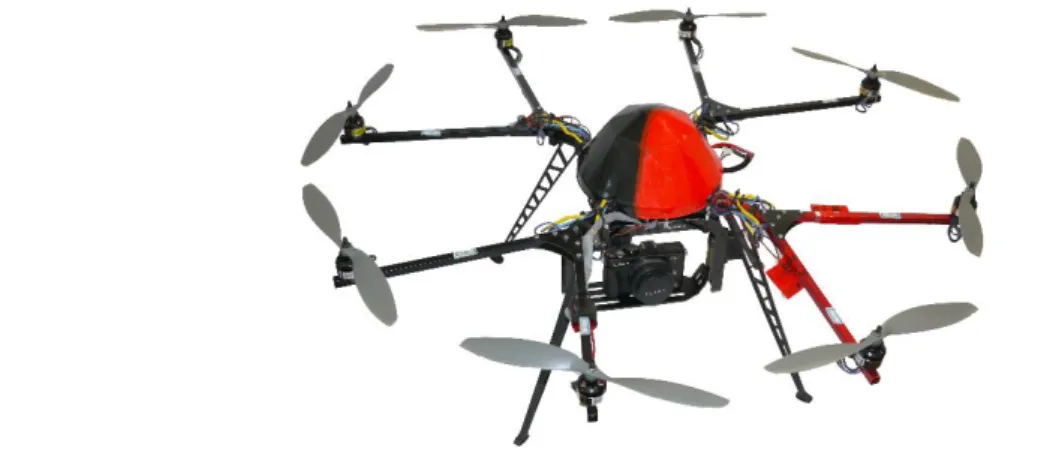
MK-OKTOKOPTER
The MK-Oktokopter, is a low cost multi-rotor platform that is available for self-assembly (HISYS- TEMS GMBH, 2013). The system consists of an aluminium and fibre reinforced plastic airframe, eight brushless motors and propellers, flight control board and navigation control board (NEITZEL AND
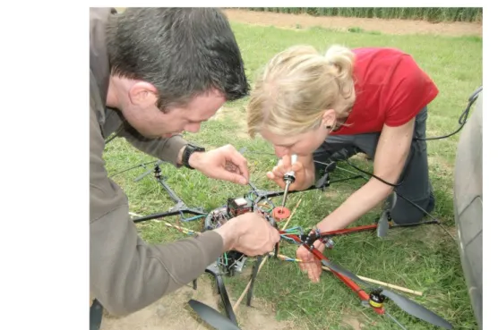
KLONOWSKI, 2011). Flight and navigation control is facilitated with high-quality gyroscopes, pres- sure sensor, compass and GPS (BÄUMKER AND PRZYBILLA, 2011). Lithium polymer batteries are used for power supply. With included batteries the UAV weighs less than 2.5 kg. The maximum addi- tional sensor payload is 1 kg. In addition to the UAV itself the UAV-system comprises a remote control and autopilot for waypoint navigation and autonomous flights (BENDIG ET AL., 2013). At- tached sensors are triggered by the remote control. Self-assembly allows for individual system modification like adding plugs to power cables for an easily detachable airframe during transport in a suitcase. Camera holder, gimbal and landing gear are adjusted according to the sensor pay- load. Furthermore, understanding the system’s principle of operation allows for onsite repair dur- ing field campaigns (Figure 2-2).
Figure 2-2: UAV-system onsite repair during one of the first field campaigns, Rheinbach, 18 May 2011.
UAVSENSORS
Today, many lightweight sensors are available for use on small UAV-systems for various crop mon- itoring applications. Sensor systems range from low-cost amateur to professional sensors specially designed for use on UAV-systems. There are visible band cameras (e.g. for 3D modelling), multi- spectral and hyperspectral ones (e.g. for crop health status) as well as thermal cameras (e.g. for plant stress). Additionally, laser scanners and radar systems are available (e.g. for 3D modelling) (COLOMINA AND MOLINA, 2014). Weight is the main limiting factor for using a sensor on a UAV.
Within the scope of this dissertation low-weight and low-cost sensors are tested on the above described MK-Oktokopter:
Visible: Panasonic Lumix GF3 and GX1 digital consumer-grade cameras (BENDIG ET AL., 2014a, 2013)
Multispectral: Tetracam Mini-MCA 4-channel multispectral camera (550, 671, 800, 950 nm) (BENDIG ET AL., 2012)
Thermal: NEC F30IS thermal imaging system (BENDIG ET AL., 2012)
Hyperspectral: Cubert UHD185 Firefly (450-950 nm) and Rikola Ltd. hyperspectral camera (500-900 nm) (BARETH ET AL., 2015)
Results presented in the following chapters concentrate on images obtained from the visible sen- sors because calibration of data from other sensors is not satisfactorily solved. The Tetracam Mini- MCA needs careful calibration and post-processing of images (KELCEY AND LUCIEER, 2012; LALIBERTE ET AL., 2011; VON BUEREN ET AL., 2014). Thermal imaging adds complexity to image interpretation due to lighting conditions, sun angle, local atmospheric conditions (BERNI ET AL., 2009b). Low image resolution (160x120 pixel for NEC F30IS) poses challenges on image georectification (HARTMANN ET AL., 2012). Cubert UHD185 Firefly and Rikola Ltd. hyperspectral camera only became available two years ago and had to be integrated in the UAV-system before first data could be recorded in 2013 (BARETH ET AL., 2015). Therefore, the following section deals with data processing of UAV- based RGB imaging only.
2.3.2 DSMs/DEMs from UAV-based RGB Imaging
Two types of models can be derived from UAV-based RGB imaging. By definition, digital surface models (DSMs) or digital terrain models (DTMs) represent the spatial distribution of terrain attrib- utes. Digital elevation models (DEMs) show the spatial distribution of elevations in an arbitrary
datum (PECKHAM AND JORDAN, 2007). Such models are needed for plant height (PH) and plant growth (PG) analysis with CSMs. The DSM/DEM generation process comprises:
image collection
image processing
and product generation.
IMAGE COLLECTION
Image collection involves considering the image scale and the area of interest (AOI). The AOI equals the agricultural field to be studied. The scale is the spatial resolution of an image. It is given by the pixel size that is the linear dimension of a pixel (ABER ET AL., 2010). The area covered by one pixel depends on the height above ground (Hg) and the focal length (f) of the camera resulting in the ground sampling distance (GSD) (Equation 2-1):
𝐺𝑆𝐷 = 𝑝𝑖𝑥𝑒𝑙 𝑠𝑖𝑧𝑒 ∗ 𝐻𝑔
𝑓 (2-1)
Images are mostly taken from a vertical vantage point, known as nadir, with a certain overlap. The minimal required forward overlap is 60% and 20-30% side lap between flight strips. Those num- bers are common in small format aerial photography (ABER ET AL., 2010). For UAV campaigns over- laps are usually higher with 80% forward overlap and 60% side lap (COLOMINA AND MOLINA, 2014).
IMAGE PROCESSING
Two types of software are generally used for image processing: traditional photogrammetry soft- ware or computer vision software. Examples for photogrammetry software are Leica Photogram- metry Suite (LPS) and PhotoModeler. The photogrammetric approach starts with camera calibra- tion, followed by ground control point (GCP) identification and tie point research either automatic or manual depending on the software (SONA ET AL., 2014). GCPs are points of known ground coor- dinates that facilitate georeferencing. Additional tie points identified by the software support the process. In a next step, exterior image orientation is estimated based on known interior image orientation. Exterior orientation is defined by X, Y and Z ground coordinates and the UAV’s roll, pitch and yaw (ABER ET AL., 2010). Roll equals the rotation around the X axis, pitch equals the rota- tion around the Y axis and yaw equals the rotation around the Z axis. Interior image orientation is defined by focal length, principal point location, three radial and two tangential distortion coeffi- cients. Finally a bundle adjustment, the orientation of an image block, is carried out (REMONDINO ET AL., 2014). Difficulties arise during image georeferencing and bundle adjustment when image positions differ from those common for classical aerial surveys. Leica LPS was initially tested on
data acquired for this study but arising problems during data processing led to a change to com- puter vision software.
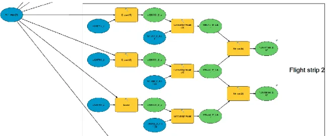
Processing with computer vision is usually faster but reduces the user’s control over georeferenc- ing and block formation as well as calculated accuracies (REMONDINO AND KERSTEN, 2012). Never- theless, results are competitive with those from the photogrammetric approach (SONA ET AL., 2014). Available software packages include Pix4UAV (Pix4D SA, Switzerland), Bundler and Agisoft PhotoScan Professional (Agisoft LLC, Russia). Agisoft PhotoScan Professional is chosen because it is easy to use and it produces high quality results (DONEUS ET AL., 2011; GINI ET AL., 2013; NEITZEL AND KLONOWSKI, 2011; SONA ET AL., 2014). Image processing with Agisoft PhotoScan is described below (Figure 2-3).
Figure 2-3: Image processing workflow with Agisoft PhotoScan.
In a first step, the images are aligned to each other. The alignment is executed using the Structure from Motion (SfM) algorithm (ULLMAN, 1979). SfM reconstructs three-dimensional scene geome- try and camera motion from an image sequence taken while moving around the scene (SZELISKI, 2010). The algorithm detects geometrical similarities like object edges, so called image feature points, and subsequently monitors their movement throughout the image sequence (VERHOEVEN, 2011). Products of the first processing step are a sparse point cloud (i), the exterior image orien- tation (ii) and the interior image orientation (iii). The sparse point cloud (i) is calculated from the information about the image feature points. Calculated camera positions equal the exterior image orientation (ii). In the photogrammetric approach (ii) and (iii) need to be known, which requires a calibrated camera. The advantage of the SfM approach with Agisoft PhotoScan is that it works with images from any uncalibrated digital camera (SNAVELY ET AL., 2008; VERHOEVEN ET AL., 2012).
Image information and thus image alignment is improved by using GCPs that are manually or half automatically identified in the images. The software’s latest version supports automatic GCP de- tection.
In a second step the detailed scene geometry is built in a bundle adjustment using dense multi- view stereo (MVS) algorithms (SCHARSTEIN AND SZELISKI, 2002). Like the image feature points, all pixels are used in this step to reconstruct finer scene details. The reconstruction accuracy may be adjusted by the user. The three dimensional geometry is then represented in a mesh of local co- ordinates. Local coordinates are transferred into an absolute coordinate system by applying a Helmert similarity transformation (VERHOEVEN ET AL., 2012).
PRODUCT GENERATION
In a third step the desired products are exported for further analysis. Products include point clouds, orthophotos and DSMs. No filtering is applied to the point clouds, thus they contain outli- ers and noise (AGISOFT LLC, 2013). Orthophotos are exported in common image formats such as
*.JPG or *.TIF with specified coordinate system, image blending mode, and the pixel size where the default value results from the entered flying height. DSM export options are similar to the latter but the default pixel size is defined by chosen accuracy during dense point cloud generation.
The DSMs are required for CSM generation (chapter 2.2).
2.4 Measuring Spectral Properties of Plants
Any RS sensor used in plant studies somehow exploits the spectral properties of plants. Tradition- ally, RS of agriculture involves timely spectral reflectance information that is linked to the plants through structural, biochemical, and physiological properties (NELLIS ET AL., 2009; ROBERTS ET AL., 2011). This section aims at explaining reflectance as well as basic concepts of vegetation indices.
Since this study focuses on biomass estimation, a more detailed description of this plant parame- ter is given.
2.4.1 Reflectance
Remote sensing methods employ electromagnetic radiation (EMR) such as light, heat and radio waves for detecting and measuring plant properties (SABINS, 1997). EMR moves at light velocity in a harmonic wave pattern in different wavelengths. Once EMR hits a matter it is either transmitted, adsorbed, scattered, emitted or reflected. Absorption causes heating and determines the EMR
emission (CAMPBELL AND WYNNE, 2011). The Stefan-Boltzmann law specifies the relationship be- tween total emitted radiation (W in watts/cm2) of a blackbody and temperature (T in K) (Equa- tion 2-2):
𝑊 = 𝜎𝑇4 (2-2)
According to this law, the total emitted radiation is proportional to temperature to the power of four, times the Stefan-Boltzmann constant (σ = 5.6697 x 10⁻⁸). The peak intensity of radiation shifts to shorter wavelengths (λ [nm]) with increased temperature (T [K]). The relationship is defined by Wien’s displacement law for a blackbody (Equation 2-3):
𝜆 = 2.897.8/𝑇 (2-3)
Short wavelength ultraviolet (UV) EMR <300 nm is absorbed by ozone (O3), and long wavelength EMR <1 cm is absorbed by clouds in the earth’s atmosphere. The atmospheric composition varies with place and time and thus EMR hitting the earth surface varies. For this study, RS methods using the reflected part of EMR are of interest.
The reflection is defined as the ratio of reflected energy to incident energy (KUMAR ET AL., 2001).
It is measured with sensors that are either framing systems, known as cameras, or scanning sys- tems, so called single detectors with a narrow field of view (FOV) (SABINS, 1997). A sensor’s spec- tral resolution is defined by the bandwidth that is determined by the wavelength interval recorded at 50% of peak response of the detector. Multispectral sensors typically consist of six to 12 broad bands whereas hyperspectral sensors consist of many (200 or more), narrow bands down to 2 nm or less (ALBERTZ, 2007; JONES AND VAUGHAN, 2010). According to the spectral resolution different plant properties can be studied.
A plant’s reflectance curve has typical properties in each spectral domain. The ranges of such do- mains are differently defined in the literature. The definition by KUMAR ET AL.(2001) is used below.
The biochemical plant constituents include foliar pigments like chlorophyll (Chl), carotene and xanthophyll that absorb light in the visible (VIS) spectrum (400-700 nm). Pigments absorb the UV and VIS with distinct but overlapping absorption features (ROBERTS ET AL., 2011). Reflectance strongly increases in the red edge between 690 and 720 nm. The point of maximum slope is called red edge inflection point. Maximum reflectance is reached at the red edge shoulder around 800 nm. The red edge position may shift due to chlorophyll concentration or LAI. Reflectance in the near-infrared (NIR) region (700-1300 nm) varies with plant species and is dominated by the leaf internal structure. The shortwave infrared (SWIR) region (1300-2500 nm) is characterized by
strong water absorption bands and a resulting lower reflectance compared to the NIR (KUMAR ET AL., 2001).
Reflectance of vegetation cover changes with the above mentioned biological aspects and the vegetation structure. Water content, age, stress, cover geometry, row spacing and orientation and leaf distribution in the cover alter vegetation reflectance (BANNARI ET AL., 1995). Furthermore, re- flectance is influenced by atmosphere composition, soil properties, soil brightness and colour as well as solar illumination geometry and viewing conditions.
2.4.2 Vegetation Indices
Vegetation indices (VIs) are developed to qualitatively and quantitatively evaluate vegetation us- ing spectral measurements in relation to agronomic parameters like biomass or PH (BANNARI ET AL., 1995). They are commonly used for extracting information from RS data (JACKSON AND HUETE, 1991). Numerous vegetation indices exist in VIS, NIR and SWIR spectral regions. The VIs are clas- sified as broad multispectral indices, narrow hyperspectral indices, and combined indices depend- ing on the width of spectral bands used for calculation. Narrow band indices can be better tuned to capture a specific absorption but need a hyperspectral sensor (MUTANGA AND SKIDMORE, 2004;
ROBERTS ET AL., 2011). Broad band indices can be calculated from many sensors. Most indices are calculated as ratios or normalized differences of two or three bands (HUNT JR. ET AL., 2013). Plant properties determined from VIs are grouped into structural, biochemical, and physiological prop- erties (ROBERTS ET AL., 2011). Structural properties include fraction of vegetation cover, green leaf biomass and leaf area index (LAI). Biochemical properties include water, pigments like chlorophyll and plant structural materials like lignin. Physiological indices measure stress-induced changes in the state of xanthophyll, chlorophyll content, fluorescence or leaf moisture (KUMAR ET AL., 2001).
VISIBLE DOMAIN VEGETATION INDICES
VIS vegetation indices (VIVIS) use the reflection in the blue (420-480 nm), green (490-570 nm) and red (640-760 nm) part of the spectrum. VIVIS can be calculated from UAV-based RGB images. Table 2-1 gives an overview of VIVIS mentioned in the literature, while VIVIS developed in this study are listed in Table 6-2. The ratio of red to green reflectance is defined as Red Green Index (RGI) or red green ratio (COOPS ET AL., 2006). The Green Red VI (GRVI) or Normalized Green Red Difference Index (NGRDI) (TUCKER, 1979) exploits the balance between red and green reflectance to distin- guish phenology stages of vegetation (MOTOHKA ET AL., 2010). The GRVI/NGRDI may also be used for biomass estimation (CHANG ET AL., 2005; HUNT JR. ET AL., 2005). The Vegetation Atmospherically
Resistant Index (VARI) has proven good estimates of leaf area index (LAI), biomass and moisture stress (GITELSON ET AL., 2003; PERRY AND ROBERTS, 2008). Moreover, it outperforms the NDVI in frac- tion of vegetation cover estimation (GITELSON ET AL., 2002). Crop parameters are assessed using the Green Leaf Index (GLI) and Triangular Greenness Index (TGI) (HUNT ET AL., 2011a) for leaf chlo- rophyll content (HUNT JR. ET AL., 2013) or NGRDI for biomass estimation (HUNT JR. ET AL., 2005). The Excess Green Index (ExG) (WOEBBECKE ET AL., 1995) quantifies green vegetation reflectance and is used for weed mapping and mapping of vegetation fraction (RASMUSSEN ET AL., 2013; TORRES- SÁNCHEZ ET AL., 2014). Although NIR VIs (VINIR) are widely used, HUNT ET AL. (2013) assert that higher correlations are found for leaf chlorophyll content and VIVIS than for VINIR.
Table 2-1: Overview of visible band vegetation indices where R = reflectance (%), RB = 450-520 nm, RG = 520-600 nm, RR = 630-690 nm, λ = reflectance at a particular wavelength (band is ± 5 nm around centre wavelength). *Multispec- tral sensor bands or digital camera bands of red, green and blue may be used instead of narrow bands (HUNT JR. ET
AL., 2013).
VI Name Formula References
RGI Red Green Index 𝑅𝑅
𝑅𝐺
(COOPS ET AL., 2006; GAMON AND SURFUS, 1999)
GRVI /NGRDI
Green Red Vegetation In- dex/
Normalized Green Red Difference Index
𝑅𝐺− 𝑅𝑅
𝑅𝐺+ 𝑅𝑅
(HUNT JR. ET AL., 2005; MOTOHKA ET AL., 2010; TUCKER, 1979)
VARI
Visible Atmospherically
Resistant Index
𝑅𝐺− 𝑅𝑅
𝑅𝐺+ 𝑅𝑅− 𝑅𝐵
(GITELSON ET AL., 2002)
GLI Green Leaf Index 2 ∗ 𝑅𝐺− 𝑅𝑅− 𝑅𝐵 2 ∗ 𝑅𝐺+ 𝑅𝑅+ 𝑅𝐵
(HUNT JR. ET AL., 2013; LOUHAICHI ET AL., 2001)
TGI* Triangular Greenness In- dex
−0.5 ((𝜆𝑟− 𝜆𝑏) − (𝑅𝑅− 𝑅𝐺))
− ((𝜆𝑟− 𝜆𝑔) − (𝑅𝑅− 𝑅𝐵))
(HUNT ET AL., 2011a)
ExG Excess Green Index 2 ∗ 𝑅𝐺− 𝑅𝑅− 𝑅𝐵
(WOEBBECKE ET AL., 1995)
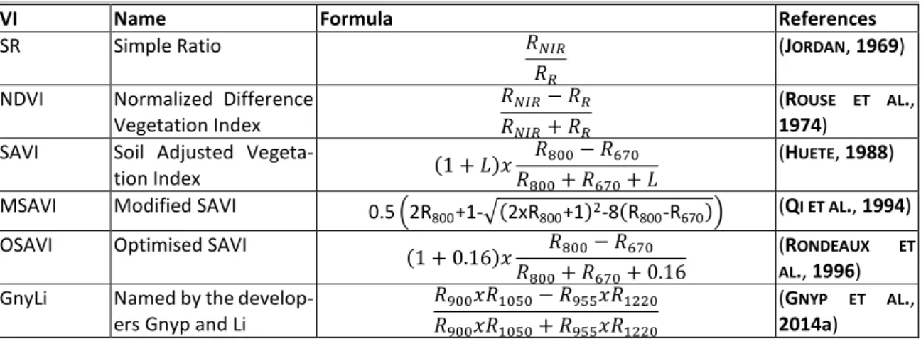
NEAR-INFRARED DOMAIN VEGETATION INDICES
Most VI equations compare an absorbing wavelength to a non-absorbing wavelength (ROBERTS ET AL., 2011). Combinations of red, green, blue and NIR or SWIR bands exist depending on the inves- tigated plant properties. Extensive lists of existing VINIR and VISWIR are given for example by BANNARI ET AL. (1995), MULLA (2013) and ROBERTS ET AL.(2011). A selection of commonly used VINIR is pre- sented in the following section (and in Table 6-1) based on the work by GNYP ET AL. (2014) and HUETE (1988). Simple Ratio (SR), the ratio of NIR to red reflectance (JORDAN, 1969) and Normalized Difference Vegetation Index (NDVI) (ROUSE ET AL., 1974) are widely used and good predictors for