Defects in strongly correlated and spin-orbit entangled quantum matter

Defects in strongly correlated and spin-orbit entangled quantum matter

Inaugural-Dissertation

zur

Erlangung des Doktorgrades

der Mathematisch-Naturwissenschaftlichen Fakultät der Universität zu Köln

vorgelegt von

Michael Becker

aus Bendorf

Köln 2014

Berichterstatter: Prof. Dr. Simon Trebst Priv.-Doz. Dr. Ralf Bulla

Tag der mündlichen Prüfung: 26. 11. 2014

Abstract

The inherent complexity of interacting quantum many-body systems poses an outstand- ing challenge to both theory and experiment. Especially in the presence of strong elec- tronic correlations, highly interesting and perplexing physical phenomena can occur.

In this thesis, we focus on three different examples of strongly correlated electron sys- tems in which different types of defects occur. First, we investigate the Heisenberg-Kitaev model formulated on a triangular lattice. Using a mixture of numerical and analytical techniques we map out the entire phase diagram for the classical and quantum models.

We provide an analytical foundation to the intriguing Z

-vortex ground state, in which strong spin-orbit coupling leads to the formation of a lattice of topological point defects.

This state was observed previously in classical Monte Carlo simulations. We furthermore propose the iridate Ba

IrTi

O

to be a prime candidate for the realization of such a state.

The second part deals with the physics of a defect in the form of a localized magnetic moment which is embedded into a metallic environment: the Kondo effect. Although this effect has been a cornerstone of condensed matter physics for more than 50 years, its properties in real-space are still not fully understood. What is the Kondo screening cloud—the extended many-body state of entangled conduction electrons? We present numerical results in 1D and 2D for the charge density oscillations created by the impu- rity. We find that the entire RG flow of the problem is recovered in these oscillations, elucidating the internal structure of the screening cloud.

Finally, we investigate the competition between the Kondo effect and Majorana

physics. Majorana bound states are highly interesting objects which exhibit unusual

statistics and could be used as a building block of a topological quantum computer. Re-

cently, signatures of their existence were observed in experiment, and we here examine

how Kondo physics (which might play a role in real systems) interact with such Majorana

bound states.

Kurzzusammenfassung

Die Komplexität wechselwirkender Quanten-Vielteilchensysteme stellt eine enorme Her- ausforderung sowohl für Theorie als auch für Experimente dar. Insbesondere in Syste- men von stark wechselwirkenden Elektronen können ungewöhnliche neue physikalische Phänomene auftreten.

In dieser Arbeit betrachten wir drei unterschiedliche Beispiele solcher stark korrelier- ter Systeme, in denen jeweils verschiedene Arten von Defekten auftreten. Als erstes wid- men wir uns dem Heisenberg-Kitaev-Modell, formuliert auf dem Dreiecksgitter. Mit nu- merischen und analytischen Methoden sind wir in der Lage, das vollständige Phasendia- gramm zu untersuchen, sowohl für das klassische als auch das quantenmechanische Mo- dell. Wir liefern eine analytische Grundlage für den Z

-Vortex-Zustand, in welchem starke Spin-Bahn-Wechselwirkung dazu führt, dass sich ein Gitter aus topologischen Punktde- fekten aufbaut. Dieser Zustand wurde kürzlich das ersten Mal in klassischen Monte-Carlo- Simulationen beobachtet. Wir schlagen vor, dass solch ein Zustand in dem Übergangs- metalloxid Ba

IrTi

O

existieren könnte.

Im zweiten Teil widmen wir uns der Physik eines Defektes in Form eines an eine metalli- sche Umgebung gekoppelten lokalen magnetischen Moments: dem Kondo-Effekt. Dieser Effekt ist seit seiner Beschreibung vor über 50 Jahren ein Grundpfeiler der Festkörper- physik. Dennoch wird die dazugehörige Physik im Ortsraum weiterhin kontrovers disku- tiert. Was genau ist die Kondo-Screening-Cloud – der örtlich ausgedehnte, verschränkte Zustand zwischen magnetischem Moment und Leitungsband-Elektronen? Wir präsentie- ren numerische Resultate für Ladungsdichte-Oszillationen in 1D und 2D, in denen wir den gesamten Renormierungsgruppenfluss des Problems wiederfinden. Damit können wir Aussagen über die innere Struktur der Screening-Cloud tätigen.

Schließlich beschäftigen wir uns mit der Frage, wie der Kondoeffekt mit der Majorana-

physik konkurriert. Gebundene Majoranazustände sind hochinteressante Objekte mit

ungewöhnlicher Statistik, die als mögliche Bausteine eines topologischen Quantencom-

puters in Frage kommen. In 2012 konnten experimentell überzeugende Hinweise auf

deren Existenz nachgewiesen werden. Wir betrachten den Einfluss des Kondoeffekts,

welcher im experimentellen Aufbau eine Rolle spielen könnte, auf solche Majoranazu-

stände.

Contents

1. Introduction 1

I. Models and numerical methods 3

2. Models of strongly correlated electrons 5

2.1. Quantum impurity problem . . . . 5

2.2. The SU(2) Heisenberg Spin Model . . . . 12

2.3. The Kitaev Honeycomb Model . . . . 13

3. Numerical methods: DMRG and NRG 19 3.1. Reducing the size of the Hilbert space . . . . 19

3.2. Matrix product states . . . . 21

3.3. Real-space renormalization . . . . 24

3.4. Density Matrix Renormalization Group . . . . 26

3.5. Numerical Renormalization Group . . . . 29

II. The Heisenberg-Kitaev model in triangular j = 1/2 Mott insulators 37 4. Transition metal oxides as j = 1/2 Mott insulators 39 4.1. Effective spin moment in transition metal oxides . . . . 39

4.2. Spin interactions . . . . 45

4.3. Kitaev interactions in real materials . . . . 47

5. The Heisenberg-Kitaev model on the triangular lattice 49 5.1. The Heisenberg model on the triangular lattice . . . . 49

5.2. The Heisenberg-Kitaev model . . . . 55

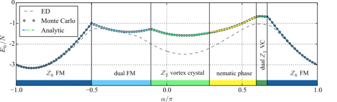
5.3. Phase diagram . . . . 58

5.4. Z

vortex lattice phase . . . . 61

5.5. Ferromagnetic order . . . . 70

5.6. Kitaev phase . . . . 74

5.7. Summary and outlook . . . . 76

III. Real-space Kondo correlations in 1D and 2D 79 6. Friedel oscillations and the Kondo screening cloud 81 6.1. Occurrence of a length scale in Kondo physics . . . . 81

6.2. The screening cloud scenario . . . . 82

6.3. Challenges to the screening cloud picture . . . . 83

6.4. Kondo length scale in charge density oscillations . . . . 84

i

ii Contents

7. 1D and Quasi-1D lattices 91

7.1. Lattice Green functions . . . . 91

7.2. Impurity Green functions . . . 101

7.3. Real-space RG flow in the charge densities . . . 102

7.4. Summary . . . 107

8. Square lattice 109 8.1. Friedel oscillations on the square lattice . . . 109

8.2. Green functions on the infinite lattice . . . 110

8.3. Impurity Green functions . . . . 113

8.4. Shape of the screening cloud . . . 116

8.5. RG flow in real space along lattice diagonals . . . 118

8.6. Summary . . . 119

IV. Kondo and Majorana interactions in quantum dots 121 9. Majorana zero modes in quantum wires 123 9.1. Kitaev’s superconducting wire . . . 124

9.2. A more realistic model: Topological superconductors . . . 124

10. Majorana fermions vs. the Kondo effect 129 10.1. The model . . . 129

10.2. Bosonization of the model . . . . 131

10.3. Renormalization group analysis and numerical results . . . 134

10.4. Results at the particle-hole symmetric point . . . 136

10.5. Summary . . . . 141

V. Appendices 143 A. Real-space Green functions from equations of motion 145 A.1. Green functions for the semi-infinite 1D chain . . . 145

A.2. Green functions for ribbons and tubes . . . 147

B. Calculations for the triangular Kitaev model 151 B.1. Lattice clusters used in the numerical calculations . . . . 151

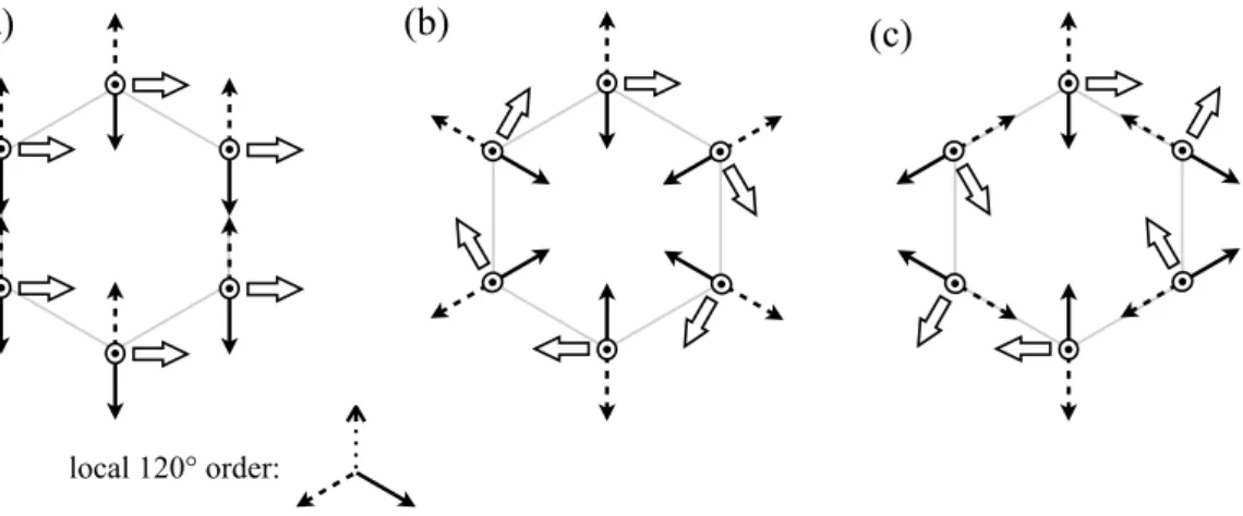
B.2. Instability of the 120

order . . . 152

B.3. Spin-wave analysis of the ferromagnet . . . 152

Acknowledgements 155

Bibliography 167

Chapter 1.

Introduction

Condensed matter systems with strong electronic correlations have brought forth some of the most remarkable physics of the last decades. From the Kondo effect, in which a single localized magnetic degree of freedom forms an entangled state with conduction electrons in its vicinity, to the physics of Mott insulators, where the strong Coulomb re- pulsion pins electrons down thereby suppressing charge transport, to spin liquids, an exotic quantum state that shows no magnetic order even at zero temperature.

Given the fact that already the Helium atom, the second-simplest element, does not allow a closed analytical solution, it is truly fascinating that physicists have been able to successfully describe and understand condensed matter systems comprised of exponen- tially many, much more complicated constituents. In these many-body systems, the indi- vidual constituents can conspire to create entirely new, emergent phenomena [1], such as fractional charges [2], heavy fermions [3], non-abelian anyons [4], or the still some- what mysterious high-T

superconductors [5]. Such physics cannot be understood con- structively from looking at a single component of the system as they are true many-body effects.

Whereas some of these systems, such as topological insulators [6] or Majorana edge states [7], can be well-described in terms of non- or weakly-interacting theories, in many other cases the strong interactions cannot be neglected. In fact, in these cases they are crucial for the occurrence of novel physics. A remarkable example is given by the physics of the so-called Mott insulators. The electrons in crystalline materials can typically travel through the system by “hopping” from one lattice site to the next. Under certain circum- stances, however, the strong Coulomb repulsion forbids two electrons to be on the same lattice site at a time, thereby effectively pinning electrons down and suppressing charge transport, and the only remaining degree of freedom is the magnetic moment of the elec- tron’s spin. These localized magnetic degrees of freedom can display a broad variety of vastly different behavior, being either magnetically ordered in a broken-symmetry state, or completely fluctuating even at zero temperature; a spin liquid state in which no sym- metry is broken. Materials and phenomena which exhibit such physics are currently one of the central research topics of both experimentalists and theorists. While this great in- terest was spurred strongly by the discovery of high-T

superconductivity in which elec- tron correlations play an important role [8], numerous other fascinating and novel phe- nomena can occur in strongly correlated systems, with a multitude of possible applica- tions in devices such as superconducting magnets or even quantum computers.

In part one of this thesis we introduce a selection of models of strongly correlated sys- tems that play a major part in the remainder of the text. Already in the simplest case of a single localized magnetic degree of freedom, historically termed an “impurity”, the highly non-trivial Kondo effect manifests: below a characteristic temperature scale, a complex many-body singlet forms and the magnetic degree of freedom is screened. This effect has witnessed a revival in the last years due to the advent of nano-scale devices such as quantum dots, allowing for accurate control of the relevant parameters and new possible

1

2 Introduction

applications of Kondo physics [9]. We present the Anderson impurity model and discuss how it leads to local moment formation and the low energy Kondo physics. Focusing then on the Mott insulators mentioned above, we present the infamous Hubbard model, a deceptively simple Hamiltonian which at present is far from fully understood [8]. Con- sidering the limit of a strong Coulomb interaction, we find the Heisenberg Hamiltonian, an effective model of the spin degrees of freedom. Finally, incorporating orbital order- ing effects, we discuss a similar model with anisotropic exchange interaction: the Kitaev model.

We then present the two numerical techniques we used extensively for the results in this thesis: the numerical renormalization group (NRG) and the density matrix renormal- ization group (DMRG). The former was devised by Kenneth Wilson in 1975 [10] and to this day is the weapon of choice for impurity problems. Almost two decades later, Steve White invented the DMRG in 1992 [11], where based on Wilson’s NRG he formulated an algorithm to calculate ground state properties of generic lattice Hamiltonians in 1D. Although both methods are typically used in very different contexts, they are born from the same ideas and can thus be considered from a common point of view.

Part two considers a model comprised of both Heisenberg and Kitaev terms, formu- lated on the triangular lattice. We discuss how in certain transition metal oxides strong spin-orbit coupling leads to a formation of a state characterized by effective j = 1/2 de- grees of freedom. Furthermore, in some of these materials, the specific exchange inter- action between these degrees of freedom might be described in terms of the Heisenberg- Kitaev model. Whereas the honeycomb version of this model has been subject of great theoretical and experimental discourse, we here focus on the triangular lattice. Thus far, only results for the classical model are known [12, 13], most of them numerical. We present a thorough analysis of the entire phase diagram, including analytical and numer- ical approaches for both the classical and quantum case.

In part three, we turn our focus to the Kondo effect. Although it has been one of the arguably most researched condensed matter topics of the 20th century [9], its real-space physics is still discussed controversially. In a broad parameter regime, an Anderson impu- rity behaves partly like a potential scatterer. This scattering induces static charge density oscillations around the impurity, known as Friedel oscillations [14]. Building on previous findings [15], we present numerical results for the Friedel oscillations in which we recover the full renormalization group flow of the impurity problem, allowing for a detailed anal- ysis of the structure of the notorious Kondo screening cloud — the quantum many-body singlet thought to be exponentially far extended in real-space.

The fourth and final part investigates the interplay between Kondo physics and Ma-

jorana bound states at the edges of quantum wires. Majorana fermions are exotic par-

ticles which are their own anti-particles. While they are conjectured to exist as possible

high-energy particles, it has become clear that they might also occur in the form of quasi-

particle excitations in condensed matter systems. In fact, in a seminal experiment, sig-

natures in transport measurements of so-called Kitaev wires have strongly indicated the

existence of Majorana bound states in these systems [16]. Although the evidence is com-

pelling, several factors might influence the results, among them disorder and the Kondo

effect. Thus, these side effects must be ruled out to achieve an unambiguous detection

of Majorana modes. We consider the interplay of Kondo and Majorana physics in an ex-

perimentally relevant setup, and show that in the experimentally relevant regimes the

low-energy physics is indeed dominated by the Majorana bound state.

Part I.

Models and numerical methods

3

Chapter 2.

Models of strongly correlated electrons

In a typical solid the intricate subtleties of quantum mechanics are combined with a vast number of ∼ 10

particles. Since these particles interact in various ways, an ex- act microscopic description of such materials seems intractable. However, it turns out that a large number of materials have properties that are comparatively insensitive to the Coulomb repulsion between electrons. In these cases, theories such as Fermi liquid theory, in which electrons are replaced by quasi-particles emerging from collective exci- tations, provide a remarkably good description of the low-temperature physics. In fact, many of the most intensively studied phenomena in condensed matter physics in recent years can be described to a significant degree in terms of non- or weakly-interacting mod- els: among them are topological insulators and superconductors [6], Majorana fermions in 1D wires [7], and graphene [17].

However, in many materials the correlations between the electrons are dominating factors and cannot be neglected. These strong correlations cannot be treated pertur- batively anymore and in many cases lead to drastically different physics! In fact, al- ready a single strongly correlated site coupled to a system of otherwise effectively non- interacting particles can give rise to such physics known as the Kondo effect, which has kept physicists busy for decades before it could finally be solved. A different example of strongly correlated systems is given by the transition metal oxides, in which the strong Coulomb correlations lead to a variety of intriguing physical phenomena, the arguably most famous one being the high-T

superconductivity discovered in doped cuprates. The unusual electronic and magnetic properties of many strongly correlated materials have also found many real-life applications such as superconducting magnets and magnetic storage [18].

In this chapter we introduce the models of strongly correlated systems considered in the main body of this thesis. This also provides a background for the discussion of nu- merical techniques in the next chapter. Starting with a non-interacting system which contains only a single site with a strong Coulomb interaction (the single-impurity Ander- son model and the Kondo model, cf. Parts III and IV), we then present the infamous Hub- bard model and its strong-coupling limit, the Heisenberg spin-Hamiltonian. Finally, we introduce the Kitaev model, a special case of a so-called compass model, which is similar to the Heisenberg model, but the spin interactions are anisotropic and depend on lattice properties (cf. Part B).

2.1. Quantum impurity problem

The arguably simplest non-trivial paradigm of a strongly correlated system is the intro- duction of a single strongly correlated impurity into an otherwise non-interacting sys- tem. Such systems are already very hard to solve and contain rich physics. The poster child of quantum impurity physics is the infamous Kondo effect: the unexpected mini-

5

6 Models of strongly correlated electrons

mum that was measured in the electronic resisitvity of gold as the temperature is low- ered. The dominant contribution to the resistivity in metals comes from the scattering of conduction electrons on phonons. As the temperature is lowered, these phonon modes are suppressed and a finite residual resistivity due to lattice defects in the metal remains.

However, in the presence of magnetic impurities, it was found [19] that below a certain temperature the resistivity increased. Thirty years later, Jun Kondo could attribute this effect to the spin-scattering of conduction electrons on the impurity spin [20] which leads to a logarithmic divergence in the resistivity below a characteristic temperature, the so- called Kondo temperature T

. Although the origin of the resistance minimum was now understood, the unphysical logarithmic divergence still posed a serious problem. A con- certed effort by many workers, especially a scaling analysis by Anderson [21], suggested that upon lowering the temperature, a local magnetic moment builds up on the impurity, and subsequently, below T

, this local moment is screened from the rest of the system by the formation of a spin-singlet state with conduction band electrons. The definitive con- firmation of this picture eventually came with Wilson’s numerical renormalization group method (NRG) [10, 22], see Chap. 3.

2.1.1. Single-impurity Anderson model

The Hamiltonian of a generic quantum impurity system can always be cast into a form consisting of three parts: the Hamiltonian of the host system, the Hamiltonian of the isolated impurity and a coupling between the two,

H = H

+ H

+ H

. (2.1)

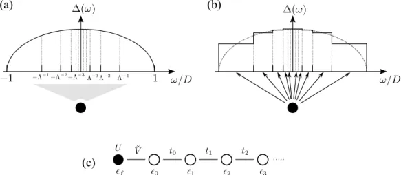
In the context of Kondo physics, the formation of a local moment on the impurity and the screening by conduction electrons can be well understood within the framework of a special quantum impurity Hamiltonian: the single-impurity Anderson model (SIAM), introduced by Anderson in 1961 [23]. In the SIAM, the host system is described by non- interacting particles and for infinite or periodic systems the Hamiltonian is diagonal in momentum space,

H

= X

kσ

ε

c

c

, (2.2)

where c

creates an electron with spin σ = ↑ / ↓ and momentum k in the conduction band, and ε

is the dispersion relation. This approach is justified by Landau’s Fermi liquid theory: At sufficiently low temperature the long-range Coulomb interaction between the electrons in the metal is screened and the effective degrees of freedom in the system can be viewed in terms of quasi-particles which move around in the host system nearly freely [3]. Neglecting the small remaining interaction between these quasi-particles turns out to be a reasonable approximation.

The second part in Eq. (2.1) is the impurity part of the Hamiltonian. In the SIAM it de- scribes a single orbital with level energy

and a Coulomb interaction U :

H

=

n ˆ

+ U n ˆ

n ˆ

, (2.3) where n ˆ

= P

σ

n ˆ

is the occupation number operator with n ˆ

= f

f

, and f

creates

an electron with spin σ on the impurity orbital. When the impurity orbital is embedded

in the host metal, the two systems are coupled via a hybridization V

. We can neglect the

k-dependence of the hybridization if the impurity couples only locally to a translationally

invariant system, and in this thesis we always assume a constant hybridization V

= V .

2.1 Quantum impurity problem 7 The Hamiltonian H

is then given by

H

= V X

σ

f

c

+ c

f

, (2.4)

where now c

=

P

k

c

(with the system’s volume V ) creates an electron in the host system orbital coupling to the impurity. Without loss of generality we can always define the origin of the host system’s coordinate system such that the hybridizing orbital is located at r = 0.

Local moment formation in the SIAM

To understand how the SIAM allows for the formation of a magnetic moment on the impu- rity, we consider the isolated impurity Hamiltonian H

. Defining | 0 i as the unoccupied impurity orbital, the impurity can be in one of the following four states, given here with their corresponding energies:

| 0 i E = 0, f

| 0 i = |↑i E =

, f

| 0 i = |↓i E =

, f

f

| 0 i = |↑↓i E = 2

+ U.

To obtain a spin doublet ground state (i.e. either |↑i or |↓i ), single occupation must be favored (

<

, where

is the Fermi energy), but the Coulomb energy must be strong enough to disfavor energetic excitations to the doubly-occupied state (

+ U >

).

Setting the Fermi level to

= 0, the requirement for the ground state to be a local magnetic moment can thus be compactly expressed as

− U <

< 0. (2.5)

In the special case when

= − U/2 the impurity is called particle-hole symmetric, as the transformation n ˆ

→ 2 − n ˆ

leaves the Hamiltonian invariant.

2.1.2. Kondo model

The SIAM provides a description of the quantum impurity system for arbitrary energies and occupation of the impurity orbital. However, we have argued that at the heart of the Kondo effect lies the spin-flip scattering on a magnetic impurity moment. Since we have identified the parameter regime in which the SIAM can sustain a local moment, we can derive an effective, simplified Hamiltonian for this special case. To this end, we project the Hamiltonian onto the subspace in which the impurity is singly-occupied. This is done via the so-called Schrieffer-Wolff transformation [24]. Taking into account virtual exci- tations to the zero- and doubly-occupied manifolds up to second order, this projection yields the following effective Hamiltonian, called the Kondo Hamiltonian:

H = H

+ K X

kk⁰σ

c

c

+ J S

· s

, (2.6)

where S

and s

are the spin-

operators for the impurity local moment and the host sys-

tem orbital spin which couples directly to the impurity. These two operators are defined

8 Models of strongly correlated electrons as

S

= X

σ,σ⁰

f

σ

f

, (2.7)

s

= X

σ,σ⁰

c

σ

c

, (2.8)

with the vector of Pauli matrices σ = (σ

, σ

, σ

). The first term H

is again given by Eq. (2.2) and the second term in Eq. (2.6) is a purely potential scattering contribution.

The effective Heisenberg exchange coupling J and the potential scattering strength K are given (to second order in V ) by [3]

J = V

1

U +

+ 1

−

, (2.9a)

K = V

2

1

−

− 1 U +

. (2.9b)

Eqs. (2.9) show that in the particle-hole symmetric case,

= − U/2, the potential scat- tering term vanishes, K = 0, and the spin interaction simplifies to

J = 4 | V |

U . (2.10)

Since the parameters U and

are constrained by Eq. (2.5), J is always positive and thus the interaction is always antiferromagnetic. This fact is an essential result as it leads to the singlet formation and screening of the impurity spin at low energies.

At this point we want to stress that the Kondo Hamiltonian in Eq. (2.6) is a low-tempera- ture effective model of the full single-impurity Anderson model defined by Eqs. (2.1)-(2.4).

Whereas the latter also describes charge fluctuations on the impurity at high energies, the former assumes a strictly singly-occupied impurity and models only the low-energy spin-spin interactions. The high-energy physics of both models differ, but the low-energy behavior and ground states of both models are identical.

2.1.3. Poor man’s scaling and the renormalization group

Having introduced two related models—the single-impurity Anderson model and its low- energy counterpart, the Kondo model—which describe a metallic host containing mag- netic impurities, we now turn to the explanation for the occurrence of the resistance min- imum. The experimentally observed correlation between the existence of a Curie-Weiß behavior in the impurity susceptibility (a local moment) and the appearance of the resis- tance minimum suggested the origin of the latter to be related to magnetic impurities.

Perturbational treatments of the Anderson and Kondo models, however, could not re- produce the minimum. Only when Kondo in 1964 [20] extended the perturbational cal- culations within the Kondo model to third order in J, the spin degeneracy of the impurity could be shown to lead to the appearance of log(T /D) terms. The resistivity is then given by

R(T ) = R

1 + 2Jρ

ln

k

T D

, (2.11)

where R

is the resistivity calculated to second order and ρ

is the density of states at the

Fermi level and k

the Boltzmann constant.

2.1 Quantum impurity problem 9

k ↑ q ↓ k

↑

↓ S ˆ

↑ S ˆ

↓

k ↑ k

↑

q ↓

↑ S ˆ

↓ S ˆ

↑

Figure 2.1.: Virtual second-order excitations into the high-energy band segments in poor man’s scaling. The thick horizontal lines represent the state of the impurity spin. The interactions with conduction band states (thin lines) flip the impurity spin, leading to a virtual excitation into the eliminated band edge (dashed line).

Subsequently, the impurity spin is flipped back into its original state. The left diagram shows the process of an electron in a quantum state | k ↑i being scat- tered into the band edge and then back into the state | k

↑i . The right diagram, on the other hand, describes the process of a particle from the band edge being scattered into the bulk of the band (leaving a hole in the band edge) and then being scattered back into the band edge.

This result finally explained the origin of the resistance minimum by attributing it to spin-spin interactions which dominate the physical processes at low enough tempera- tures. Unfortunately, it also implied the divergence of all physical quantities for T → 0.

The problem of how to extend the calculations to the regime T T

attracted the at- tention of many theorists and quickly became known as the Kondo problem. It could eventually be overcome with the help of the poor man’s scaling technique developed by Anderson in 1970 [21]. In this approach the band width is progressively reduced, and second-order virtual excitations to the band edges are eliminated perturbatively. In each step, an energy interval of size δD is cut off from the band at the edges. The reduced band thus runs from ( − D + | δD | ) → (D −| δD | ). Excitations to the eliminated states are taken into accout perturbatively, and it turns out that the only non-trivial contributions arise from virtual second-order excitations into the high-energy intervals and back. Fig. 2.1 shows diagrammatic representations of these processes.

Once the band width is reduced, the resulting Hamiltonian has exactly the same form as the original. However, the coupling parameters are renormalized J → J ˜ and the Hamiltonian is now defined on a reduced bandwidth 2 ˜ D = 2(D − | δD | ). The reduction step is then applied repeatedly, and in the limit of infinitesimally small energy intervals,

| δD | → dD, yields a differential equation for the coupling parameter J , viz.

dJ

d ln(D) = − 2ρ

J

+ O ρ

J

. (2.12)

This differential equation defines a flow of the coupling parameter as the tempera- ture/energy scale is progressively reduced. Integrating Eq. (2.12) we find a so-called scaling invariant of the Kondo effect, the Kondo temperature T

:

D exp

− 1 ρ

J

= ˜ D exp

− 1 ρ

J ˜

∼ T

. (2.13)

The invariance of T

under the reduction of the energy scale implies that, for low enough

temperatures, all properties of the system must depend only on this parameter T

. A

10 Models of strongly correlated electrons

better estimate of T

is obtained from perturbation theory to third order, giving T

= D p

ρ

J exp

− 1 ρ

J

. (2.14)

The renormalization group

Building on the scaling ideas by Anderson discussed in the previous section, we can formulate the more general concept of the renormalization group (RG) method, which was largely pioneered in the context of critical systems in condensed matter physics by Kadanoff [25] and Wilson [10]. It is a mapping R of a Hamiltonian H(K) which is spec- ified by a set of coupling parameters K = (K

, K

, . . .), into a new Hamiltonian of the same form but with different (renormalized) coupling parameters K, formally: ˜

R(K) = ˜ K. (2.15)

The series of points K defines trajectories in parameter space, also called the RG flow (in the sense that these trajectories have a direction and are smooth). Typically, the trans- formation R consists of integrating out local (microscopic) degrees of freedom in order to eventually obtain a description of the system on a macroscopic level. An example for such a transformation was given in the last subsection by the reduction of the band width. Other examples include Wilson’s real-space renormalization group procedure (see Chap. 3), and the Kadanoff block spin transformation in which the RG scheme consists of an explicit coarse-graining of space. Both these schemes are discussed in more detail in Ref. [10].

A key concept within the RG framework is that of fixed points. A fixed point is a point K

where the RG transformation leaves the coupling parameters invariant,

R(K

) = K

. (2.16)

At these points, further application of the RG scheme will not change the description of the system anymore. One generally distinguishes between stable and unstable fixed points. The trajectories in the vicinity of a stable fixed point are drawn towards it—the system flows to the stable fixed point. In the neighborhood of an unstable fixed point, however, trajectories are eventually driven away and flow to the stable fixed point.

2.1.4. Fixed Points of the RG flow

Applying the renormalization group idea to the symmetric flat-band Anderson model renormalizes the parameters U → U ˜ and V → V ˜ . We find three distinct fixed points [3, 22], and in Fig. 2.2 we show the RG flow diagram for the symmetric Anderson model.

The three fixed points can be interpreted in a physically intuitive way:

Free orbital (FO): At high temperatures, T ∼ D, charge fluctuations to and from the impurity are dominant and the system is described by the (unstable) free orbital fixed point. At this fixed point, the impurity can be in all four possible states. The charge fluctuations lead to peaks in the impurity density of states ρ

() at =

and =

+ U , which are commonly known as the Hubbard satellites.

Local moment (LM): Lowering the temperature (or energy scale) by applying the RG

scheme iteratively, below a certain energy scale charge fluctuations are frozen out

2.1 Quantum impurity problem 11

H

H

H

D

Ũ

Ṽ D

Figure 2.2.: Renormalization group flow of the symmetric Anderson model [3]. The only stable fixed point is the strong coupling fixed point at V

→ ∞ . The red line in- dicates the RG flow shared with the Kondo model where only the local moment and strong coupling fixed points are present. In the Kondo model, J ∼ V

/U is the renormalized parameter.

and the impurity orbital becomes singly-occupied, forming a local magnetic mo- ment. The system flows away from the FO fixed point to the (unstable) local mo- ment fixed point. In the RG flow the LM fixed point lies at U ˜ → ∞ . In this regime, the Kondo model serves as an adequate low-energy theory of the Anderson model.

Accordingly, the Kondo model with J = 0 (cf. Eqs. (2.10)) is described by the same LM fixed point.

Strong coupling (SC): Further lowering the temperature, as soon as the Kondo temper- ature scale at T

is reached, spin-scattering processes become dominant and the formation of the Kondo singlet groundstate is represented by the system flowing to the stable strong-coupling fixed point. In the impurity density of states the forma- tion of the singlet leads to a narrow peak of width T

around the Fermi level: The so-called Kondo resonance. The SC fixed point is the V

= ∞ limit of the Anderson model, and accordingly the J = ∞ limit of the Kondo model.

Fig. 2.3 shows the impurity entropy in the single-impurity Anderson model as a function of ω for three different sets of impurity parameters. At high energies, ω ∼ D, the system is at the FO FP, and the four possible states of the impurity yield an entropy S

= log(4) = 2 log(2). At a non-universal energy scale, the impurity degrees of freedom reduce to that of a single spin-

, and S

= log(2). Finally, below the Kondo scale the impurity is screened, the resulting singlet state has an entropy of S

= log(1) = 0.

2.1.5. The Kondo resonance

The spin exchange between the conduction electrons and the localized impurity spin

qualitatively change the energy spectrum of the system [9]. The combined scattering

processes generate a new state, known as the Kondo resonance, at the Fermi level

.

This new state also substantiates the intuitive picture we have established so far: the

electrons mainly contributing to the low-temperature conductivity of a metal have ener-

gies around the Fermi level. Since the Kondo resonance also forms at the Fermi energy,

12 Models of strongly correlated electrons

SC LM FO

T

Figure 2.3.: Impurity entropy in the single-impurity Anderson model as a function of ω for three different sets of impurity parameters. The data was obtained with the Numerical Renormalization Group for a constant hybridization function, and the parameters of the Anderson model were

/D = − 0.8 × 10

, V /D = 3 × 10

and U/D = 1 × 10

, 1.125 × 10

and 1.25 × 10

(solid, dashed, and dotted lines).

it is precisely these electrons that are affected most, leading naturally to an increased resistivity. Various experimental measurements of the Kondo resonance [26, 27] have recently been obtained by measuring the linear-response conductance G and the differ- ential conductance dI/dV through a quantum dot, which was tuned to form a spin-

impurity.

2.2. The SU(2) Heisenberg Spin Model

In the previous section we considered the case of a system of non-interacting fermions coupled to a single impurity—a localized orbital with strong Coulomb interaction. The description of a metal in terms of a Fermi liquid, i.e. non-interacting fermionic quasipar- ticles, is a vital approach that has proven to be very successful in many cases. However, when electron-electron interactions become dominant this description is not useful any- more. The physics of such strongly correlated electrons is, in fact, a bona fide example of the inapplicability of Fermi liquid theory [8].

2.2.1. Hubbard model

A very fruitful starting-point for the description of such systems is given by the Hubbard model; a deceptively simple tight-binding Hamiltonian with only on-site interactions. It has been proposed by J. Hubbard in 1963 to understand the physics of transition metal monoxides [28], but it has since been applied to many different systems and problems, e.g. heavy fermions [3] and high-T

superconductivity [29]. It has been attacked with the full range of analytic and numerical techniques available to condensed matter theorists, but in spite of its simplicity it is at present far from being completely understood [8]. The Hubbard-Hamiltonian is given by

H

= − t X

hiji,σ

c

c

+ U X

i

ˆ

n

n ˆ

, (2.17)

2.3 The Kitaev Honeycomb Model 13 where c

creates an electron with spin σ at lattice site i, and ˆ n

= c

c

is the occu- pation number operator. The first term describes the hopping of electrons between two nearest-neighbor sites i and j, with the hopping amplitude t. The second term represents the strong Coulomb interaction between two electrons on the same site.

2.2.2. Mott insulators and Heisenberg Hamiltonian

One of the many successes of the Hubbard model was the description of Mott insulators:

materials that under conventional band theory are expected to be conducting, however show insulating behavior in experiment. The explanation of this discrepancy in terms of strong interactions between electrons follows immediately from the Hubbard model.

Starting from the Hubbard Hamiltonian in Eq. (2.17) at half-filling (i.e. an electron con- centration of on average one electron per lattice site), we examine the effect of inter- actions. To this end, we consider the dimensionless interaction parameter U/t. In the weakly interacting limit, U/t 1, one can resort to standard Fermi liquid theory and the interaction term in Eq. (2.17) can be viewed as a mere perturbation to the non-interacting system. In the opposite limit of U/t 1, however, the electrons in the system will be localized at each site. The immense energy penalty from the Coulomb repulsion is thus avoided at the expense of the (much smaller) kinetic energy t. In this case charge carriers cannot travel through the system and the system becomes insulating; this is known as a Mott insulator [30]. The groundstate of the half-filled Hubbard model for U t is thus a system where each site is occupied by one electron, carrying a spin-

. To derive an ef- fective theory for this situation we treat the hopping of electrons in perturbation theory, and integrating out second-order virtual excitations into intermediate states in which a site becomes doubly-occupied yields the Heisenberg spin-Hamiltonian:

H

= J X

hiji

S

· S

, (2.18)

where S

= (S

, S

, S

) is the vector of spin-

operators at site i, and J = 2t

U . (2.19)

The interaction in Eq. (2.18) is antiferromagnetic, since J > 0. The origin of this fact can be explained very simply [8]: For two neighboring sites occupied with electrons of parallel spin, an intermediate state of both electrons on one site is strictly forbidden by the Pauli principle. The same process is allowed, though, for electrons of anti-parallel spin. In the latter case, such a process leads to an energy gain of ∆E = − 2t

/U .

2.3. The Kitaev Honeycomb Model

The interaction terms in the Heisenberg model are isotropic, i.e. symmetry operations of the underlying lattice do not change the Hamiltonian. Now, we discuss a special model with anisotropic interactions, i.e. where the relative spatial alignment of two interacting spins determines the type of interaction. This model was first presented by A. Kitaev in 2006, after he had found an exact solution to it [31] while considering it in the context of fault-tolerant quantum computation.

Not only is the fact that an exact solution to a (non-trivial) 2D model exists remarkable

by itself, this so-called Kitaev model furthermore possesses an abundance of compelling

14 Models of strongly correlated electrons

y x z

(a) (b)

y x z

y x

z

↵

Figure 2.4.: (a) The honeycomb lattice of the Kitaev model. Each site belongs to one of two sublattices, shown here as empty or filled disks. The gray diamond shows the unit cell containing two sites. (b) A graphical representation of the Majorana fermionization. The large gray bubbles represent a spin-

and each black dot represents one Majorana fermion.

physical properties: It can be solved by mapping to non-interacting Majorana fermions, its ground state is a true quantum spin liquid with topological order [32], and it contains both abelian and non-abelian anyonic excitations in the presence of a magnetic field.

At the time of Kitaev’s original publication it was not clear how to realize this model in a real system [31]. Recently, however, Khaliullin and co-workers suggested [33] that the Kitaev model might be in part realized in certain transition metal oxide systems with or- bital degrees of freedom. This discovery spurred a lot of research and is one of the main motivations for the problems considered in this thesis (see Part II). In the following, we present the model along with a sketch of the solution.

2.3.1. The model

The Kitaev model consists of spin-

degrees of freedom located at the vertices of a honey- comb lattice, Fig. 2.4(a). The lattice can be subdivided into two sublattices with the unit cell containing two sites. Interactions occur between nearest-neighbor spins and are di- vided into three types depending on the direction of the link between the sites. Each type of interaction is an Ising-like coupling of one spin component and we call them “x-links”,

“y-links” and “z-links”, see Fig. 2.4(a). The full Hamiltonian is given by H

= J

X

x−links

S

S

+ J

X

y−links

S

S

+ J

X

z−links

S

S

, (2.20)

with three independent coupling parameters J

, J

and J

. As the honeycomb lattice

is bipartite there is no geometrical frustration when considering only nearest-neighbor

interactions. However, it is the anisotropic spin-interaction terms that highly frustrate

the model. To see this, consider one spin interacting with its three neighbors: for each

individual neighbor, the spin minimizes its energy by aligning along a different spin axis,

which cannot be fulfilled with respect to all three neighbors at the same time.

2.3 The Kitaev Honeycomb Model 15 2.3.2. Majorana fermions

The Dirac equation as a relativistic generalization of the Schrödinger equation describes all spin-

particles (such as electrons) as well as their anti-particles (such as positrons).

Whereas in general particles and their anti-particles are different, Ettore Majorana showed in 1937 [34] the existence of a solution of the Dirac equation which is its own anti-particle. This is most easily seen in terms of operators where the Majorana solution is a linear combination of two “regular” Dirac-fermions. Consider the fermionic operator c

(c

) that destroys (creates) a Dirac particle and obeys the canonial anticommutation relation { c

, c

} = δ

. From this, we can construct the following linear combination:

γ

= 1

√ 2

c

+ c

, γ

= 1

√ 2i

c

− c

. (2.21)

These new operators γ

are purely real solutions to the Dirac equation. They are thus hermitian and also obey fermionic statistics

{ γ

, γ

} = δ

, γ

= γ

. (2.22) Eq. (2.22) shows explicitly that the Majorana fermions are indeed their own anti-particle.

From Eqs. (2.21) we furthermore see that we can express a regular Dirac fermion as the combination of two Majoranas as

c

= 1

√ 2 (γ

+ iγ

) , c

= 1

√ 2i (γ

− iγ

) . (2.23) In its original paper, Ettore Majorana speculated that his findings might apply to neu- trinos, which at that time were themselves only hypothetical. Remarkably, more than 80 years later, it is to this day still not certain whether neutrinos are in fact Majorana fermions or not [35]. Furthermore, the theory of supersymmetry in high energy physics also has put forth candidates for Majorana fermions, such as the so-called weakly inter- acting massive particles (WIMPs) in the context of dark matter [36].

In the field of condensed matter physics, the search for Majorana fermions has recently attracted much interest as it was suggested that they occur as quasiparticle excitations in a variety of systems. Although the use of Majorana fermions in condensed matter theory is mostly motivated from a purely mathematical standpoint [35], the possibility of real materials exhibiting such physics leads to a realistic chance of further exploring and even utilizing their exotic features.

We discuss how the Kitaev model can be solved in terms of Majorana fermion operators in the following sections, and in Part IV we focus on a different system at the center of the current search for Majorana fermions.

2.3.3. Representation of spins by Majorana fermions

Following Kitaev’s original solution, we employ the Majorana fermions initially as a math- ematical tool which turns out to be essential for the solution of the Kitaev model. To this end, we represent one spin at site i by four Majorana fermions which we call α

, β

, β

, and β

. The spin operators can now be written in terms of these Majoranas as

S

= iβ

α

, (2.24)

16 Models of strongly correlated electrons

J _x

J _y J _z

A

B A A

Figure 2.5.: Phase diagram of the Kitaev model. Shown is a cut at J

+ J

+ J

= const through the positive octant. The gapped phase A and the gapless phase B are discussed in the main text. The other octants have equivalent phase diagrams.

where γ ∈ { x, y, z } . Fig. 2.4(b) gives a graphical representation of this transformation. A side-effect of this mapping is that with the introduction of the Majorana operators we doubled the Hilbert space. This, however, can be remedied by restricting the Hilbert space to its physical sector, which can be done by requiring the new spin operators to fulfill the spin SU(2) algebra. In the Majorana representation, the Kitaev Hamiltonian Eq.

(2.20) becomes

H = i 4

X

hiji

J

iβ

β

| {z }

=ˆuij

α

α

, (2.25)

where the sum runs over nearest-neighbors h ij i and, as before, γ ∈ { x, y, z } corre- sponds to the type of link. Remarkably, the operators u ˆ

commute with each other and the Hamiltonian, and we can therefore split the Hilbert space into eigenspaces of each ˆ

u

which are indexed by their eigenvalues ± 1. Replacing the operators u ˆ

by their eigen- values u

yields a Hamiltonian quadratic in the Majorana modes. This non-interacting problem is then exactly solvable.

2.3.4. Spectrum and phase diagram

The freedom of fixing every u

leaves us with the question which configuration mini- mizes the ground state energy? In fact, from a theorem by Lieb [37] it follows that the ground state is achieved by a field configuration where u

= 1 for all links where j be- longs to the even sublattice, and k to the odd sublattice. This configuration obviously has a translational symmetry and we find the fermionic spectrum by Fourier transformation of the operators in the Hamiltonian

H = i 4

X

hiji

J

u

α

α

. (2.26)

The spectrum is then readily found as ε(k) = ± 4

J

e

+ J

e

+ J

, (2.27)

2.3 The Kitaev Honeycomb Model 17 with the two lattice vectors of the honeycomb lattice a

= (

,

√3

2

) and a

= ( −

,

√3 2

).

From here, we can immediately identify the parameter regime in which the spectrum is gapless (i.e. a solution exists for ε(k) = 0), which is the case exactly when the following three triangle inequalities are fulfilled

| J

| ≤ | J

| + | J

|

| J

| ≤ | J

| + | J

|

| J

| ≤ | J

| + | J

| .

We call the gapless phase B , and the gapped phases A, and show them in Fig. 2.5 for a cut through the parameter space for which J

+ J

+ J

= const.

2.3.5. Spin liquid ground states

A remarkable property of the Kitaev model was first elucidated in Ref. [32]: In its ground state, dynamical two spin correlation functions are short ranged and vanish exactly be- yond nearest-neighbor separation, independent of the values of J

, J

and J

. Therefore, the ground state, in both phases A and B, is given by a short-ranged quantum spin liquid with no long range spin order [38].

In the phase A the spin liquid is gapped and has a Z

topological order. In fact, in the limit that one coupling is much stronger than the two others, e.g. J

, J

J

, the Hamiltonian can be mapped to the toric code [31], a thoroughly studied model of a topo- logical quantum error correcting code [39]. The phase B, on the other hand, is gapless, and it contains quasi-particle excitations in the form of non-abelian anyons, objects of tremendous interest in the context of topological quantum computation, see also Part IV.

Thus, the combination of an exact solution and the great number of rich physics, such

as the non-abelien anyonic excitations in the gapless spin liquid state, have made this

model a central focus of theoretical and experimental condensed matter research in re-

cent years.

Chapter 3.

Numerical methods: DMRG and NRG

Strongly-correlated many-body quantum systems on low-dimensional lattices present a challenging task for both analytical and numerical treatment. The presence of strong interactions leads to failure of perturbation theory. Field-theoretic approaches have led to great insights but oftentimes rely on severe approximations. Numerically, a lattice system of finite size can in principle always be solved exactly by means of diagonaliza- tion. However, the Hilbert space of the problem grows exponentially in system size and thus severely restricts the system sizes feasible for simulation to the order of currently O (10). Although computational power steadily increases, this exponential barrier can- not be overcome and one has to turn to approximate solutions.

Kadanoff’s block spin renormalization group was a first major step to understanding how to successfully apply renormalization group ideas from other fields in condensed matter physics. In his paper [25], he shows a way to define components of the theory at large distances by iterative aggregation of components at shorter distances. By group- ing spins into blocks and then transforming the system so that each group of spins is now represented by a single effective spin, one effectively “zooms out” of the system and eventually reaches a description of the long length scale (or, conversely, low-energy) physics. This approach was further corroborated by Kenneth G. Wilson while working on the Kondo problem, and led to the invention of the numerical renormalizaton group (NRG) algorithm [10]. However, the concepts and ideas that enabled the NRG to be to this day the most powerful weapon to tackle Kondo physics fail for essentially all many-body lattice systems. Even a single free particle in a box cannot be described by Wilsons’s ap- proach. Eventually, Steven R. White realized that an important change in the approach was needed to enable it to treat general one-dimensional lattice systems to great accu- racy. In 1992 he invented the density matrix renormalization group (DMRG) technique [11] which since then has proven to be the most powerful numerical method for one- dimensional systems know to date. Recently, with a deeper understanding of the un- derlying mathematical and physical structures, and the growth in computational powers available, the DMRG algorithm could be extended to also treat 2D systems (however only systems of small width).

Although the problems for which NRG and DMRG are best suited are very different, and although both algorithms have strongly differing features, at their core they are in- timately related. In this chapter, we introduce both techniques from the point of view of their common foundation and in the modern language of matrix product states.

3.1. Reducing the size of the Hilbert space

The Hilbert space of a quantum lattice system comprised of N sites with a local Hilbert space of dimension d is exponentially large with a dimension D = d

. However, it turns out that not the entire Hilbert space is required to describe the ground state of a realistic

19

20 Numerical methods: DMRG and NRG

Hamiltonian, and renormalization group methods for many-body systems (see Chap. 2.1) have the goal to identify precisely the relevant degrees of freedom of a given system. To this end, it is important to better understand how we can reduce the full Hilbert space to a relevant sub-manifold.

3.1.1. Entanglement entropy

How much a state is spread throughout the full Hilbert space can be quantified by means of the entanglement entropy. Consider a system X which is comprised of two subsys- tems A and B such that X = A ∪ B. Assuming this system to be in a pure state | ψ i , the entanglement entropy is defined as the von Neumann entropy of either subsystem (since it is the same for either subsystem). First, we can formulate the reduced density matrices for each subsystem by tracing out the other subsystem,

ˆ

ρ

= Tr

| ψ i h ψ | , ρ ˆ

= Tr

| ψ i h ψ | . (3.1) The operators ρ ˆ

and ρ ˆ

have the same eigenvalues, λ

, and by applying iteratively a singular value decomposition (SVD) [40] the full state | ψ i can be written in the so-called Schmidt decomposition as

| ψ i = X

i

λ

| a i

⊗ | b i

, (3.2)

where | a i

and | b i

are eigenvectors of ρ

and ρ

, respectively. This formulation is re- lated to the matrix product states we discuss below, where a state is written in terms of tensor products of local objects. From the spectrum of the reduced density matrices one can now rigorously define the entanglement entropy as

S = Tr ρ

log ρ

= − X

i

λ

log λ

. (3.3) If | ψ i is a non-entangled state, the density matrices only have one non-vanishing eigen- value which—due to normalization—is λ

= 1, and accordingly the entanglement en- tropy vanishes, S = 0. On the other hand, a maximally entangled state will have an ex- ponentially large number of equal eigenvalues, leading to the (maximal) entanglement entropy S = log D.

3.1.2. Area laws

At first glance, one might argue that a calculation of the entanglement spectrum must be performed in the full Hilbert space and we have thus gained nothing. However, one can prove for one-dimensional systems and certain two-dimensional systems that low- energy eigenstates of gapped Hamiltonians with local interactions obey so-called area laws for the entanglement entropy [41, 42]. In particular, the entanglement entropy of the ground states of such systems grows proportionally to the surface of the cut rather than the subsystem’s volume. Taking for instance the two subsystems A and B as in Fig.

3.1, we find S(A) ∼ ∂A = L + W . For a 1D system, this in fact implies S

= S

= const.

It is important to stress that the fact that most systems have an area law leads to dra-

matic consequences, as it heavily constrains the number of possible candidates for the

ground state in the Hilbert space. Indeed, the manifold of states with an entanglement

entropy that grows with boundary rather than volume makes up only an exponentially

small part of the full Hilbert space [40,43]. Therefore, by reducing the Hilbert space of the

3.2 Matrix product states 21

A B

W

L

W

Figure 3.1.: Subsystems A and B comprising the full system X = A ∪ B. If the system obeys an area law, the entanglement entropy of subsystem A grows with the boundary between A and B, S

∼ W + L, and not with the volume of A, S

∼ W · L.

problem to the relevant manifold of states obeying an area law, we can massively reduce the required computational resources.

In fact, it turns out [44] that using the formalism of matrix product states (or more gen- erally tensor networks), which we describe below, one automatically targets exactly such states. Accordingly, when constructing numerical RG methods to focus on the most rele- vant degrees of freedom, it is natural to formulate them in the context of matrix product states.

3.2. Matrix product states

To introduce the formalism of matrix product states, consider a lattice of L sites where each site has a local Hilbert space of dimension d. While the following discussion is valid for arbitrary dimensions of the system, for our purposes we assume the lattice to be one- dimensional. Any pure state of this system can be formulated as

| ψ i = X

σ1,...,σL

c

| σ

i | σ

i . . . | σ

i , (3.4) where the sum runs over all d

states in the full Hilbert space and we have an exponen- tially large number of coefficients c

. A matrix product state is a representation of this state by means of local objects, where the coefficients c

are expressed in terms of matrices A

as

c

= A

A

. . . A

A

. (3.5) and thus the state | ψ i is given in a matrix product state formulation by

| ψ i = X

σ1,...,σL

A

A

. . . A

A

| σ

i | σ

i . . . | σ

i . (3.6)

At this point, of course, this is a mere reformulation and the number of total coefficients

is naturally still exponentially large. In fact, the dimensions of the matrices A grow ex-

ponentially, where A

is a (1 × d) matrix, A

is (d × d

), and so forth. The dimensions

grow for the first half of the matrices, then they decrease in the same manner until finally

A

is a (d

× d) matrix, and A

is a (d × 1) vector. Thus, for a practical (numerical)

treatment we have gained nothing so far.

22 Numerical methods: DMRG and NRG

To see how we can reduce the level of complexity by finding an optimal approximation, consider again the Schmidt decomposition in Eq. (3.2). From the reasoning above we know that for only slightly entangled states, only a few density matrix eigenvalues λ

contribute most of the weight. By summing only over the M largest eigenvalues λ

in Eq. (3.2), we can thus create an approximate state | ψ ˜ i ≈ | ψ i , and it can be shown [40]

that this is in fact an optimal approximation.

Turning back to the matrix product states we can in the same fashion limit the max- imum matrix dimension of the matrices A

to be M d

. The matrix size yields an upper bound for the rank of the reduced density matrices, and in this sense takes on the same role as the M in the Schmidt decomposition. By keeping only the largest M sin- gular values in each decomposition, we can thus approximate the state | ψ i with a set of matrices A

where each matrix is at most of dimension (M × M ).

3.2.1. Matrix Product Operators (MPO)

With the representation of arbitrary states as matrix product states, we now turn to the representation of operators. In the basis of the MPS states, {| σ

i} , we can write any op- erators as [40]

O ˆ = X

σ1,...,σL

X

σ₁⁰,...,σ_L⁰

W

W

. . . W

0 L−1

L−1

W

| σ i h σ

| , (3.7) where we have introduced the notation for a basis state

| σ i ≡ | σ

i | σ

i . . . | σ

i . (3.8) The W

in Eq. (3.7) are matrices just like the matrices A

in Eq. (3.6) with the only dif- ference that they depend on not one but two external indices, σ and σ

, which can be understood as ingoing and outgoing physical states. The coefficients of the operator are then readily obtained as

h σ | O ˆ | σ

i = W

W

. . . W

0 L−1

L−1

W

0 L

L

. (3.9)

The application of an MPO to an MPS follows straight-forwardly from their definitions:

O ˆ | ψ i = X

σσ⁰

W

W

. . . W

A

A

. . . W

| σ i

= X

σ

N

N

. . . N

| σ i , (3.10) where the new matrices N

have the multiplied dimension of the MPS and the MPO.

Noteably, the form of the MPS stays invariant at the prize of an increased matrix size.

In typical applications, however, the new MPS can be truncated again to the original matrix dimensions. The operation of summing over exponentially many basis vectors

| σ

, σ

, . . . , σ

i has been reduced to a polynomial operation, of order Ld

D

M

where D

is the dimension of the MPO [40].

3.2.2. Graphical representation of MPS and MPO

While generally the usage of MPS requires a lot of notational overhead, a much more con-

venient diagrammatic notation exists. From this point, we use the general word tensor