GI-Edition
Lecture Notes in Informatics
Dietmar Schomburg, Andreas Grote (Eds.)
German Conference on Bioinformatics 2010
September 20 - 22, 2010 Braunschweig, Germany
D . Sc homburg, A. Grote (Eds.): GCB 2010
Proceedings
publishes this series in order to make available to a broad public recent findings in informatics (i.e. computer science and informa- tion systems), to document conferences that are organized in co- operation with GI and to publish the annual GI Award dissertation.
Broken down into
• seminar
• proceedings
• dissertations
• thematics
current topics are dealt with from the vantage point of research and development, teaching and further training in theory and prac- tice. The Editorial Committee uses an intensive review process in order to ensure high quality contributions.
The volumes are published in German or English.
Information: http://www.gi-ev.de/service/publikationen/lni/
This volume contains papers presented at the 25 th German Conference on Bioin- formatics held at the Technische Universität Carolo-Wilhelmina in Braunschweig, Germany, September 20-22, 2010. The German Conference on Bioinformatics is an annual, international conference, which provides a forum for the presentation of current research in bioinformatics and computational biology. It is organized on behalf of the Special Interest Group on Informatics in Biology of the German Society of Computer Science (GI) and the German Society of Chemical Technique and Biotechnology (Dechema) in cooperation with the German Society for Bio- chemistry and Molecular Biology (GBM).
173
ISSN 1617-5468
ISBN 978-3-88579-267-3
German Conference on Bioinformatics 2010
September 20-22, 2010
Technische Universität Carolo Wilhelmina zu Braunschweig, Germany
Gesellschaft für Informatik e.V. (GI)
Volume P-173
ISBN 978-3-88579-267-3 ISSN 1617-5468
Volume Editors
Prof. Dr. Dietmar Schomburg
Technische Universität Carolo-Wilhelmina zu Braunschweig Email: d.schomburg@tu-bs.de
Dr. Andreas Grote
Technische Universität Carolo-Wilhelmina zu Braunschweig Email: andreas.grote@tu-bs.de
Series Editorial Board
Heinrich C. Mayr, Universität Klagenfurt, Austria (Chairman, mayr@ifit.uni-klu.ac.at) Hinrich Bonin, Leuphana-Universität Lüneburg, Germany
Dieter Fellner, Technische Universität Darmstadt, Germany Ulrich Flegel, SAP Research, Germany
Ulrich Frank, Universität Duisburg-Essen, Germany
Johann-Christoph Freytag, Humboldt-Universität Berlin, Germany Thomas Roth-Berghofer, DFKI
Michael Goedicke, Universität Duisburg-Essen Ralf Hofestädt, Universität Bielefeld
Michael Koch, Universität der Bundeswehr, München, Germany Axel Lehmann, Universität der Bundeswehr München, Germany Ernst W. Mayr, Technische Universität München, Germany Sigrid Schubert, Universität Siegen, Germany
Martin Warnke, Leuphana-Universität Lüneburg, Germany Dissertations
Dorothea Wagner, Universität Karlsruhe, Germany Seminars
Reinhard Wilhelm, Universität des Saarlandes, Germany Thematics
Andreas Oberweis, Universität Karlsruhe (TH)
Gesellschaft für Informatik, Bonn 2010
printed by Köllen Druck+Verlag GmbH, Bonn
Preface
This volume contains papers presented at the 25th German Conference on Bioinformat- ics held at the Technische Universit¨at Carolo-Wilhelmina in Braunschweig, Germany, September 20-22, 2010. The German Conference on Bioinformatics is an annual, in- ternational conference, which provides a forum for the presentation of current research in bioinformatics and computational biology. It is organized on behalf of the Special Interest Group on Informatics in Biology of the German Society of Computer Science (GI) and the German Society of Chemical Technique and Biotechnology (Dechema) in cooperation with the German Society for Biochemistry and Molecular Biology (GBM).
Five outstanding scientists were invited to give keynote lectures to the conference:
• Edda Klipp - ‘Cellular stress response and regulation of metabolism’
• Thomas Lengauer - ‘HIV Bioinformatics: Analyzing viral evolution for the ben- efit of AIDS patients’
• Werner Mewes - ‘The data deluge: can simple models explain complex biological systems?’
• Stefan Schuster - ‘Road games in metabolism - A biotechnological perspective’
• Gregory Stephanopoulos - ‘After a decade of systems biology, time for a record card’
Besides the keynote lectures, the scientific program comprised 22 contributed talks presenting 12 regular and 10 short papers. All accepted regular papers are collected in these proceedings. The remaining accepted contributions, i.e. short papers and poster abstracts, are published in a separate volume. We would like to thank the pro- gram committee members and all reviewers for their evaluations of the contributions.
Furthermore, we would like to thank the local organizers for keeping the conference running. The organizers are grateful to all the sponsors and supporting scientific part- ners. Last but not least, we would like to thank all contributors and participants of the GCB 2010.
Braunschweig, August 2010
Dietmar Schomburg and Andreas Grote
5
Organizers
Conference Chair
Dietmar Schomburg, Braunschweig
Local Organizers
Wolf-Tilo Balke (TU Braunschweig) S´andor Fekete (TU Braunschweig) Reinhold Haux (TU Braunschweig) Dieter Jahn (TU Braunschweig) Frank Klawonn (Ostfalia University of Applied Sciences)
Constantin Bannert (TU Braun- schweig)
Antje Chang (TU Braunschweig)
Andreas Grote (TU Braunschweig) Katharina Hanke (TU Braun- schweig)
Adam Podstawka (TU Braun- schweig)
Alexander Riemer (TU Braun- schweig)
Maurice Scheer (TU Braunschweig)
Programm committee
Mario Albrecht, Saarbr¨ucken Wolf-Tilo Balke, Braunschweig Tim Beißbarth, G¨ottingen Thomas Dandekar, W¨urzburg S´andor Fekete, Braunschweig Georg F¨ullen, Rostock Robert Giegerich, Bielefeld Reinhold Haux, Braunschweig Ralf Hofest¨adt, Bielefeld Matthias Heinemann, Z¨urich Dieter Jahn, Braunschweig Frank Klawonn, Wolfenb¨uttel Edda Klipp, Berlin
Ina Koch, Berlin
Oliver Kohlbacher, T¨ubingen Thomas Lengauer, Saarbr¨ucken Hans-Peter Lenhof, Saarbr¨ucken
Michael Marschollek, Hannover Werner Mewes, M¨unchen
Michael Meyer-Hermann Frankfurt Burkhard Morgenstern, G¨ottingen Stefan Posch, Halle
Matthias Rarey, Hamburg Falk Schreiber, Gatersleben Stefan Schuster, Jena
Gregory Stephanopoulos, Cam- bridge USA
Jens Stoye, Bielefeld Andrew Torda, Hamburg Martin Vingron, Berlin Christian von Mering, Z¨urich Edgar Wingender, G¨ottingen Andreas Ziegler, L¨ubeck
6
Sponsors and supporters
Supporting scientific societies
Gesellschaft f¨ur Chemische Technik und Biotechnologie e.V.
(DECHEMA)
http://www.dechema.de
Gesellschaft f¨ur Biochemie und Molekularbiologie e.V. (GBM) http://www.gbm-online.de
Gesellschaft f¨ur Informatik e.V. (GI) http://www.gi-ev.de
Non-profit sponsors
Technische Universit¨at Braunschweig http://www.tu-braunschweig.de
Commercial sponsors
Biobase - Biological Databases http://www.biobase-international.com
CLC bio
http://www.clcbio.com
Convey Computer
http://www.conveycomputer.com genomatix
http://www.genomatix.de
7
MEGWARE Computer Cluster http://www.megware.com Thalia
http://www.thalia.de Transtec - IT & Solutions http://www.transtec.de
8
Table of Contents
Preface 5
Organizers 6
Sponsors and supporters 7
Table of Contents 9
Submissions 11
Andreas R. Gruber, Stephan H. Bernhart, You Zhou, Ivo L. Ho- facker
RNALfoldz: efficient prediction of thermodynamically stable, local secondary structures . . . 11 Florian Battke, Stephan K¨orner, Steffen H¨uttner, Kay Nieselt
Efficient sequence clustering for RNA-seq data without a reference genome . 21 Florian Bl¨ochl, Maria L. Hartsperger, Volker St¨umpflen, Fabian J.
Theis
Uncovering the structure of heterogenous biological data: fuzzy graph parti- tioning in the k-partite setting . . . 31 Sergiy Bogomolov, Martin Mann, Bj¨orn Voß, Andreas Podelski, Rolf Backofen
Shape-based barrier estimation for RNAs . . . 41 Thomas Fober, Marco Mernberger, Gerhard Klebe, Eyke H¨ullermeier Efficient Similarity Retrieval of Protein Binding Sites based on Histogram Comparison . . . 51 Peter Husemann, Jens Stoye
Repeat-aware Comparative Genome Assembly . . . 61 Katrin Bohl, Lu´ıs F. de Figueiredo, Oliver H¨adicke, Steffen Klamt, Christian Kost, Stefan Schuster, Christoph Kaleta
CASOP GS: Computing intervention strategies targeted at production im- provement in genome-scale metabolic networks . . . 71 Jan Grau, Daniel Arend, Ivo Grosse, Artemis G. Hatzigeorgiou, Jens Keilwagen, Manolis Maragkakis, Claus Weinholdt, Stefan Posch Predicting miRNA targets utilizing an extended profile HMM . . . 81
9
Jan Budczies, Carsten Denkert, Berit M. M¨uller, Scarlet F. Brockm¨oller, Manfred Dietel, Jules L. Griffin, Matej Oresic, Oliver Fiehn
METAtarget – extracting key enzymes of metabolic regulation from high- throughput metabolomics data using KEGG REACTION information . . . . 103 Andreas Gogol-D¨oring, Wei Chen
Finding Optimal Sets of Enriched Regions in ChIP-Seq Data . . . 113 Enrico Glaab, Jonathan M. Garibaldi, Natalio Krasnogor
Learning pathway-based decision rules to classify microarray cancer samples . 123
Index of authors 135
10
RNALfoldz: efficient prediction of thermodynamically stable, local secondary structures
Andreas R. Gruber 1 , Stephan H. Bernhart 1 , You Zhou 1,2 , and Ivo L. Hofacker 1
1 Institute for Theoretical Chemistry
University of Vienna, W¨ahringerstraße 17, 1090 Wien, Austria
2 College of Computer Science and Technology Jilin University, Changchun 130012, China {agruber, berni, ivo}@tbi.univie.ac.at, zyou@jlu.edu.cn
Abstract: The search for local RNA secondary structures and the annotation of unusu- ally stable folding regions in genomic sequences are two well motivated bioinformatic problems. In this contribution we introduce RNALfoldz an efficient solution two tackle both tasks. It is an extension of the RNALfold algorithm augmented by sup- port vector regression for efficient calculation of a structure’s thermodynamic stability.
We demonstrate the applicability of this approach on the genome of E. coli and investi- gate a potential strategy to determine z-score cutoffs given a predefined false discovery rate.
1 Introduction
Over the past decade noncoding RNAs (ncRNAs) have risen from a shadowy existence to one of the primary research topics in modern molecular biology. Today computational RNA biology faces challenges in the ever growing amount of sequencing data. Effi- cient computational tools are needed to turn these data into information. In this context, the search for locally stable RNA secondary structures in large sequences is a well mo- tivated bioinformatic problem that has drawn considerable attention in the community.
RNALfold [HPS04] has been the first in a series of tools that offered an efficient solution to this task. Instead of a straight-forward, but costly sliding window approach a dynamic programming recursion has been formulated that predicts all stable, local RNA structures in O(N × L 2 ), where L is the maximum base-pair span and N the length of the sequence.
Since its publication, the RNALfold algorithm has inspired a lot of work in this field, see
e.g. Rnall by Wan et al. [WLX06] or RNAslider by Horesh et al. [HWL + 09]. All
contributions so far in this field focused on improving the computational complexity of
the algorithm, but none of the approaches has ever been used to unravel results of biolog-
ical significance. In particular, de novo detection of functional RNA structures has been
addressed, but application on a genome-wide scale with a low false discovery rate seems
still out of reach. Even on the moderately sized genome of E. coli (4.6 Mb) one is drown-
ing in hundreds of thousands of local structures. Unlike in the well established field of
protein coding gene detection where one can exploit signals like codon usage, functional
RNA secondary structures, in general, do not show strong characteristics that make them easily distinguishable from random decoys. Successful approaches for ncRNA detection operating solely on a single sequence [HHS08, JWW + 07] are limited to specific RNA classes, where some outstanding characteristics can be harnessed. There is no master plan for the detection of functional RNA structures, but one would certainly want to limit the RNALfold output to a reasonable amount. So far, only the minimum free energy (MFE) of the locally stable secondary structures, which is intrinsically computed by the algorithm, has been considered as potential discriminator to limit the number of secondary structures.
As demonstrated clearly by Freyhult and colleagues [FGM05] the MFE is roughly a func- tion of the length of the sequence and the G+C content. Even normalizing the MFE by length of the sequence does not serve as a good discriminator between shuffled or coding sequences and functional RNA structures. A strategy that does work, however, is to com- pare the native MFE E of the RNA molecule to the MFEs of a set of shuffled sequences of same length and base composition [LM89]. This way we can evaluate the thermodynamic stability of the secondary structure. A common statistical quantity in this context is the z-score, which is calculated as follows
z = E − µ σ
where µ and σ are the average and the standard deviation of the energies of the set of shuffled sequences. The more negative the z-score the more thermodynamically stable is the structure. Efficient estimation of a sequence’s z-score has been a profound problem already addressed in the very beginnings of computational RNA biology. A first strategy to avoid explicit shuffling and folding was based on table look-ups of linear regression coefficients [CLS + 90]. Clote and colleagues [CFKK05] introduced the concept of the asymptotic z-score, where the efficient calculation is also solved via table look-ups. The current state-of-the art approach for fast and efficient estimation of the z-score is to use support vector regression [WHS05].
The study by Clote and colleagues and a follow up to Chen et al. (1990) [LLM02] also report on the effort to predict thermodynamically stable structures using a sliding window approach. In this contribution we present RNALfoldz an algorithm that combines local RNA secondary structure prediction and the efficient search for thermodynamically stable structures. RNALfoldz is an extension of the RNALfold algorithm augmented by sup- port vector regression for efficient calculation of a sequence’s z-score. We demonstrate the applicability of this approach on the genome of E. coli and investigate a potential strategy to determine z-score cutoffs given a predefined false discovery rate.
2 Methods
2.1 Fast estimation of the z-score using support vector regression
For the efficient estimation of the z-score we follow the strategy first introduced by Washietl
et al. [WHS05]. Instead of explicit generation and folding of shuffled sequences in order to
determine the average free energy and the corresponding standard deviation support vector regression (SVR) models are trained to estimate both values. As described in detail in the previous work, we used a regularly spaced grid to sample sequences for the training set.
Synthetic sequences ranged from 50 to 400 nt in steps of 50 nt. The G+C content, A/(A+T) ratio and C/(C+G) ratio were, however, extended to a broader spectrum, now ranging from 0.20 to 0.80 in steps of 0.05. A total of 17,576 sequences were used for training. For each sequence of the training set 1,000 randomized sequences were generated using the Fisher- Yates shuffle algorithm, and subsequently folded with RNAfold with dangling ends op- tion -d2 [HFS + 94]. SVR models for the average free energy and standard deviation were trained using the LIBSVM package ( www.csie.ntu.edu.tw/˜cjlin/libsvm ).
While in the previous work input features and the dependent variables were normalized to a mean of zero and a standard deviation of one, we apply here a different normalization strategy that leads to a significantly lower number of support vectors for the final models.
For the regression of the average free energy model the dependent variable is normalized by the length of the sequence, while for the standard deviation it is the square root of the sequence length. The length still remains in the set of input features and is scaled from 0 to 1. Other features remain unchanged. We used a RBF kernel, and optimized values for the SVM parameters were determined using standard protocols for this purpose. Final regres- sion models were selected by balancing two criteria: (i) mean absolute error (MAE) on a test set of 5,000 randomly drawn sequences of arbitrary length (50-400) from the human genome, and (ii) complexity of the model (number of support vectors) , which translates to following procedure: from the top 10% of regression models in terms of MAE we selected the one that had the lowest number of support vectors. For the average free energy re- gression we selected a model with a MAE of 0.453 and 1,088 support vectors, and for the standard deviation regression a model with a MAE of 0.027 and 2,252 support vectors. To validate our approach we finally compared z-scores derived from the SVR to traditionally sampled z-scores on a set of 1,000 randomly drawn sequences from the human genome.
The correlation coefficient (R) is 0.9981 and the MAE is 0.072. This is in fair agreement to results obtained when comparing two sets of sampled z-scores (R: 0.9986, MAE: 0.054, number of shuffled sequences = 1,000).
2.2 Adaption of the RNALfold algorithm
RNALfold computes locally stable structures of long RNA molecules. It uses a Zuker type secondary structure prediction algorithm [ZS81] and restricts the maximum base pair span to L bases to keep the structures local. The sequence is processed from the 3’ (the sequence length n) to the 5’ end. In order to keep the number of back trace operations low and the output at moderate size, we want to avoid backtracing structures that differ only by unpaired regions. Furthermore, only the longest helices possible are of interest. To achieve this, a structure starting at base i is only traced back if the total energy F (i, n) is smaller than that of its 3’ neighbor F (i + 1, n) while its 5’ neighbor has the same energy:
F (i−1, n) = F (i, n) < F (i+1, n). The local minimum structure is found by identifying
the pairing partner j of i so that C(i, j) + F (j + 1, n) = F (i, n), i.e. the minimum energy
from i to n is decomposed into the local minimum part i, j and the rest of the molecule.
Here, C(i, j) stands for the energy of a structural feature enclosed by the base pair i, j.
As a result of this, the output of RNALfold contains components, i.e. structures that are enclosed by a base pair, only. Before we actually start the trace back, we evaluate two new criteria: (1) the sequence of the structure traced back has to be within the training parameters of the SVR, and (2) the z-score of the energy of this structure has to be lower than a predefined bound. Criterion (1) is simply imposed by the training boundaries of the SVMs. Boundaries have, however, been chosen carefully to cover a broad range of today’s known spectrum of functional RNA structures. 99.79% of the sequences in the Rfam v. 10 full data set match the base composition requirements of the SVR and 90% of Rfam RNA families are in within the sequence length restrictions.
In order to get the exact sequence composition that is needed for the SVR evaluations, the 3’ end of the structure (j ) has to be computed first. This is done by a first, short backtracing step, where the decomposition F (i, n) = C(i, j) + F (j + 1, n) is used to find j. Subsequently, the average free energy given the base composition of the sequence s(i, j) is computed by calling the corresponding SVR model. The SVR model for the standard deviation has approximately twice the number of support vectors as the average free energy model. To minimize calls of this model, first the minimal standard deviation for the particular sequence length is looked up. We can then, using the free energy of C(i, j), calculate a lower bound of the z-score. Only if this lower bound is below the minimal required z-score, the support vector regression for the standard deviation is called to calculate the actual z-score. If the z-score then still meets the minimal z-score criterion, the structure is fully traced back and printed out.
3 Results
The concept of fast and efficient estimation of the z-score by support vector regression was first introduced by Washietl et al. [WHS05], and implemented in the noncoding RNA gene finder RNAz. The speed up of this approach compared to explicit shuffling and fold- ing, which is usually done on 1,000 replicas, is tremendous, at minimum a factor of 1,000.
Moreover, computing time is invariant to the length of the sequence, while RNA folding is of complexity of O(N 3 ). When considering the z-score as evaluation criterion in the RNALfold algorithm, calculation of the z-score becomes a time consuming factor, as in a worst case scenario it has to be done almost for every nucleotide of the sequence. It is therefore a crucial concern to use support vector models that do not only have good accu- racy, but also a moderate number of support vectors (SVs). In this work we extended the z-score support vector regression to cover a broader range of the sequence spectrum, but managed at the same time to build models that have significantly less SVs than the models used by RNAz. This was accomplished by normalizing the dependent variables of the re- gression, i. e. the average free energy and the standard deviation, by the sequence length.
The dependent variables do not strictly linearly correlate with the sequence length and so
we have to keep the sequence length as an input feature. Nevertheless, redundant points
are created in the training set, which eventually leads to a smaller space to be trained. For
the average free energy model and the standard deviation model we were able to achieve a 6.3 and a 2.7 fold reduction, respectively, in the number of SVs compared to the RNAz equivalents.
3.1 Evaluation of RNALfoldz predicition accuracy
For the task of predicting local RNA secondary structures one would particularly be inter- ested in following criteria: (i) to which extent can functional ncRNAs be discovered, (ii) how well do the molecule’s predicted boundaries match to the real coordinates, and (iii) is there any significant difference between native, biological sequences and random decoys.
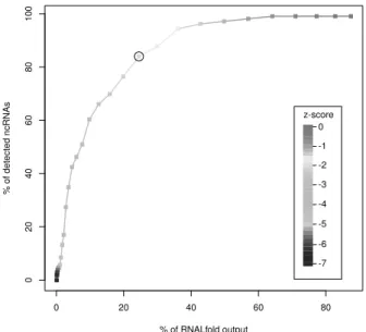
To address these questions, we applied RNALfoldz to the genome of E. coli (Accession number: CP000948). A maximum base-pair span L of 120 nt and a z-score cutoff of -2 was used. Setting the cutoff at -2 is for sure restrictive, but it should still cover a large fraction of the ncRNA repertoire. Both strands were considered. A total of 202,126 structures have been obtained. In comparison, the regular RNALfold returned a total of 1,387,136 structures, 824, 000 of which have a length ≥ 50 nt. The RNALfoldz output (a true subset of the RNALfold output) is only a forth of the regular RNALfold output.
The E. coli genome Genbank file lists 119 ncRNAs with a maximum length of 120 nt in its current annotation. To investigate the extent annotated ncRNAs are covered in the RNALfoldz output, we define for a RNALfold/RNALfoldz prediction to be counted as hit a minimal coverage of 90% of the ncRNA sequence. Giving this setup a total of 106 and 89 ncRNAs can be found in the RNALfold and RNALfoldz output, respectively.
Detailed results for each RNA gene are shown in an online supplementary table. With a z-score cutoff of -2, 17 ncRNAs that were found by RNALfold are not in output set of RNALfoldz. The detection success is directly proportional to the reduction rate of the RNALfold output. Modulating the z-score cutoff affects both quantities (Fig. 1). The failure to detect the 13 ncRNAs that were missed by both RNALfold and RNALfoldz results from the fact that the RNALfold algorithm predicts only self-contained RNA structures. For example, the two ncRNA genes rprA and ryeE that have only low cover- ing RNALfoldz hits, have indeed multi-component structures at the MFE level (abstract shape notation [GVR04]: [][][][], [][][]). In these cases RNALfoldz will rather produce multiple hits than one single hit covering the whole ncRNA. Overall, our findings confirm that most E. coli small ncRNAs are indeed more thermodynamically stable than expected by chance and that the RNALfoldz algorithm is able to detect these structures efficiently.
We further investigated how precisely the RNALfoldz predictions map to the coordinates
of the annotated ncRNAs. This is a legitimate issue, but one has to keep in mind that
functional RNAs adopt their structure at the transcription level, while in this experiment
we used the genomic sequence to detect these structures. So it might easily happen that
the RNA is predicted in a bigger structural context than its actual size. The underlying
dynamic programming algorithm is the same for RNALfold and RNALfoldz, and hence
results discussed here do hold for both versions. In this work we define noise as the fraction
of the RNALfoldz hit that does not overlap with the annotated ncRNA. In total, 34 out of
0 20 40 60 80
020406080100
% of RNALfold output
%ofdetectedncRNAs 0
-7 z-score
-6 -5 -4 -3 -2 -1
Figure 1: Non-coding RNA detection success vs. reduction of the RNALfold output. Given a z- score cutoff of 0 only one structure prediction is missed in the RNALfoldz output. With a z-score cutoff of -2 (circle) we see a four-fold reduction of the output, while at the same time covering 84%
of the correct RNALfold ncRNA predictions.
the 89 predictions have less than 10% noise. Averaged over all hits ( ≥ 90% coverage) we see noise of 18%. Using a classic sliding window approach with a length of 120 nt, one would expect more than 33% noise for a window containing a tRNA sequence (average length of tRNAs in E. coli: 78 nt). In the RNALfoldz output we find that 29 out of 73 tRNA predictions have less than 10% noise.
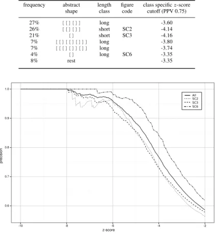
Finally, we address the significance of the predictions when compared to randomized con- trols. Therefore, we performed the same experiment on randomized sequences generated by (i) mononucleotide shuffling, (ii) simulation with an order-0 Markov model (mononu- cleotide frequencies) , and (iii) simulation with an order-1 Markov model (dinucleotide frequencies). Shuffling and simulations were done with shuffle from Sean Eddy’s squid library using default parameters. A detailed comparison of the results of these four experiments is shown in Fig. 2. In general, we observe a tendency to more stable structures in the native sequence than in any randomized sequence. Structures with a z-score ≤ -8 are profoundly enriched in the native sequence, which might point to biological relevance of these structures. These are, however, extremes and most ncRNAs will have z-score values in a much higher range.
The value -2 for the z-score cutoff in this experiment was chosen arbitrarily. Moving to an
even lower value than -2 will reduce the false discovery rate, but at the same time limit the
number of ncRNAs that show such high thermodynamic stability. Using the RNALfoldz
output from the experiment with randomized sequences (order-1 Markov model), we can
calculate an empirical precision or positive predictive value (PPV), which is simply the
native mononucleotide shuffled
order-0 Markov model
order-1 Markov model
z-score
Figure 2: Comparison of the distribution of stable secondary structures from the native E. coli genome and randomized controls. The native E. coli sequence has a strong tendency to more stable local secondary structures. RNALfoldz predictions with a z-score below -8 are exclusively found in the native sequence.
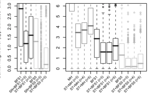
proportion of true positives against all positive results. Assuming that thermodynamic sta- bility is inherently linked to biologically function, we declare any RNALfoldz prediction with a z-score below a certain threshold from the native sequence and the randomized se- quence as true positive and as false positive, respectively. Using then a PPV of 0.75, which corresponds to 25% estimated false positives, and, hence, a deduced z-score cutoff of - 3.86 we can find 25 of the 106 annotated ncRNAs that are detectable with the RNALfold algorithm, while reducing the RNALfoldz to 21,715 predictions (3% of the RNALfold output). We further investigated if we can determine more specific z-score cutoffs when the RNALfoldz output is partitioned into different structural classes. This is motivated by the reasonable assumption that, for example, a short stable hairpin is more likely formed by chance than a stable, structurally more complex, multi-branched molecule. Hence, one would set different z-score cutoffs for different structural classes. To investigate this claim we map the MFE structures to the corresponding abstract RNA shape at the highest ab- straction level. At this abstraction level only the helix nesting pattern is considered. As an example, the well-known cloverleaf structure of tRNA molecules is then simply repre- sented as [[][][]]. The six major structural classes are shown in Tab. 1. We further partition structures according to their length into two classes short (≤ 85 nt) and long.
Fig. 3 shows structure class specific precision values in dependency of the z-score, for
those three classes that show the most deviation from the population precision. Using
now class-specific z-score values when filtering the RNALfoldz output we can raise our
prediction count from 25 to 38 ncRNAs, while keeping the expected false-positive rate
fixed at 25%. The total number of RNALfoldz predictions increases slightly to 23,225.
Table 1: Major structural classes in the E. coli genome
frequency abstract length figure class specific z-score shape class code cutoff (PPV 0.75)
27% [[][]] long -3.60
26% [[][]] short SC2 -4.14
21% [] short SC3 -4.16
7% [[][[][]]] long -3.80
7% [[[][]][]] long -3.74
4% [] long SC6 -3.35
8% rest -3.35
AllSC2 SC6 SC3
Figure 3: Precision values of different structural classes by the z-score. The solid line represents the whole RNALfoldz output.
3.2 Timing
The overall complexity O(N × L 2 ) of the core algorithm does not change, the z-score calculation just adds a constant factor. We benchmarked both implementations on an Intel Quad Core2 CPU with 2.40 GHz. Detailed results are shown in Tab. 2.
At a maximal base-pair span of 120 nt RNALfold is able to scan at a speed of approx.
250 kb/min. At the same settings and with a minimal z-score cutoff of -2 scanning speed
drops to 153 kb/min for RNALfoldz. The performance clearly depends on the number
of times the support vector regression has to be called. When moving to a lower z-score
cutoff of -4 the scanning speed increases to 207 kb/min.
Table 2: Timing results [sec] for RNALfold and RNALfoldz.
L RNALfold RNALfoldz
z-score ≤ -2 z-score ≤ -3 z-score ≤ -4
120 1,123 1,842 1,477 1,359
240 2,629 3,922 3,321 3,105
4 Discussion
In this work we have presented an extension of the RNALfold algorithm to predict ther- modynamically stable, local RNA secondary structures. Using fast support vector regres- sion models to calculate the z-score this approach comes with only a minor overhead in execution time compared to the former version, while yielding at the same time a much lower number of relevant structures. We have demonstrated that already with a z-score cutoff of -2, approx. 80% of the annotated E. coli small ncRNAs can be found in the RNALfoldz output. Comparison to randomized genome sequences showed that the na- tive E. coli genome sequence has a strong bias to more stable secondary structures. This shift is, however, not significant enough to qualify RNALfoldz as a stand-alone RNA gene finder with an acceptable false discovery rate. We see the role of RNALfoldz mainly as a first filtering step in a cascade of computational ncRNA detection steps. In particular, the intersection of data from high throughput sequencing, promoter and tran- scription termination signals (see e.g. [SNS + 10]) or G+C content on AT rich genomes with RNALfoldz hits could be of value.
In this contribution, we assume that thermodynamic stability is inherently coupled to bi- ological function. This is certainly true to some extent, but there are also a lot of RNA classes where stability is not a major issue for function, e.g. C/D box snoRNAs or ncR- NAs that form interaction with other RNAs. It is therefore highly unlikely that these RNA classes will show up in the RNALfoldz output. In this context, RNALfoldz can, how- ever, be used to define a set of highly stable loci which can then be excluded from further analysis.
It has been noted early on that thermodynamic stability alone is not a sufficient discrim- inator to distinguish ncRNAs from random sequences [RE00]. This is the main reason why most ncRNA gene finders rely solely on signals from evolutionary conservation of RNA secondary structures, or use thermodynamic stability only as an additional feature.
These methods are clearly limited by the comparative genomics data available. Investiga- tion of species that are distantly related to any species sequenced so far, or species specific RNA genes are, hence, out of scope for these methods. The RNALfoldz algorithm pre- sented in this work will not be a magic tool suddenly shedding light on these dark areas.
The search for extraordinarily stable structures, however, can help to give first clues to
putatively functional RNA secondary structure elements, where other methods fail.
Acknowledgments
This work has been funded, in part, by the Austrian GEN-AU projects “bioinformatics integration network III”
and “regulatory non-coding RNAs”. RNALfoldz is part of the Vienna RNA package and can be obtained free of charge at: http://www.tbi.univie.ac.at/˜ivo/RNA/ . An electronic supplement located at http:
//www.tbi.univie.ac.at/papers/SUPPLEMENTS/RNALfoldz compiles training and test data.
References
[CFKK05] P Clote, F Ferr´e, E Kranakis, and D Krizanc. Structural RNA has lower folding energy than random RNA of the same dinucleotide frequency. RNA, 11(5):578–591, 2005.
[CLS
+90] J H Chen, S Y Le, B Shapiro, K M Currey, and J V Maizel. A computational procedure for assessing the significance of RNA secondary structure. Comput Appl Biosci, 6(1):7–
18, 1990.
[FGM05] E Freyhult, P P Gardner, and V Moulton. A comparison of RNA folding measures.
BMC Bioinformatics, 6:241–241, 2005.
[GVR04] R Giegerich, B Voss, and M Rehmsmeier. Abstract shapes of RNA. Nucleic Acids Res, 32(16):4843–4851, 2004.
[HFS
+94] I L Hofacker, W Fontana, P F Stadler, L S Bonhoeffer, M Tacker, and P Schuster. Fast Folding and Comparison of RNA Secondary Structures. Monatsh. Chem., 125:167–
188, 1994.
[HHS08] J Hertel, I L Hofacker, and P F Stadler. SnoReport: computational identification of snoRNAs with unknown targets. Bioinformatics, 24(2):158–164, 2008.
[HPS04] I L Hofacker, B Priwitzer, and P F Stadler. Prediction of locally stable RNA secondary structures for genome-wide surveys. Bioinformatics, 20(2):186–190, 2004.
[HWL
+09] Y Horesh, Y Wexler, I Lebenthal, M Ziv-Ukelson, and R Unger. RNAslider: a faster engine for consecutive windows folding and its application to the analysis of genomic folding asymmetry. BMC Bioinformatics, 10:76–76, 2009.
[JWW
+07] P Jiang, H Wu, W Wang, W Ma, X Sun, and Z Lu. MiPred: classification of real and pseudo microRNA precursors using random forest prediction model with combined features. Nucleic Acids Res, 35(Web Server issue):339–344, 2007.
[LLM02] S Y Le, W M Liu, and J V Maizel. A data mining approach to discover unusual folding regions in genome sequences. Knowledge-Based Systems, 15(4):243 – 250, 2002.
[LM89] S Y Le and J V Maizel. A method for assessing the statistical significance of RNA folding. J Theor Biol, 138(4):495–510, 1989.
[RE00] E Rivas and S R Eddy. Secondary structure alone is generally not statistically significant for the detection of noncoding RNAs. Bioinformatics, 16(7):583–605, 2000.
[SNS
+10] J Sridhar, S R Narmada, R Sabarinathan, H Y Ou, Z Deng, K Sekar, Z A Rafi, and K Rajakumar. sRNAscanner: a computational tool for intergenic small RNA detection in bacterial genomes. PLoS One, 5(8), 2010.
[WHS05] S Washietl, I L Hofacker, and P F Stadler. Fast and reliable prediction of noncoding RNAs. Proc Natl Acad Sci U S A, 102(7):2454–2459, 2005.
[WLX06] X F Wan, G Lin, and D Xu. Rnall: an efficient algorithm for predicting RNA local secondary structural landscape in genomes. J Bioinform Comput Biol, 4(5):1015–1031, 2006.
[ZS81] M Zuker and P Stiegler. Optimal computer folding of large RNA sequences using
thermodynamics and auxiliary information. Nucleic Acids Res, 9(1):133–148, 1981.
Efficient sequence clustering for RNA-seq data without a reference genome
Florian Battke 1†∗ , Stephan K¨orner 1† , Steffen H¨uttner 2 , Kay Nieselt 1
1 Center for Bioinformatics, University of T¨ubingen, Germany
2 H¨olle & H¨uttner AG, Derendinger Str. 40, 72072 T¨ubingen, Germany
† equally contributing authors battke@informatik.uni-tuebingen.de
Abstract: New deep-sequencing technologies are applied to tran- script sequencing (RNA-seq) for transcriptomic studies. However, current approaches are based on the availability of a reference ge- nome sequence for read mapping. We present Passage, a method for efficient read clustering in the absence of a reference genome that allows sequencing-based comparative transcriptomic studies for currently unsequenced organisms. If the reference genome is available, our method can be used to reduce the computational ef- fort involved in read mapping. Comparisons to microarray data show a correlation of 0.69, proving the validity of our approach.
1 Background
Changes in transcription are the most important mechanism of differenti- ation and regulation. Until recently, the transcriptional activity of a cell was measured by PCR in the case of few genes, or microarrays were used to investigate the whole transcriptome of an organism or tissue. Both meth- ods require previous knowledge about the organism’s transcripts, either in the form of ESTs or a complete reference genome sequence for primer resp. probe design. SAGE (serial analysis of gene expression) [VZVK95]
is a method to study transcriptional activity based on sequencing of short transcript fragments. The advent of new deep sequencing technologies (also called next-generation or second generation sequencing methods) now allows to study the transcriptome in unprecedented detail by directly sequencing the pool of expressed transcripts. Using RNA-seq [WGS09]
and a known reference genome, transcriptional activity can be measured with single-base precision.
Sequencing the pool of expressed transcripts creates millions of short (36-
500 bases) sequences, called reads. These need to be mapped against
the reference genome sequence allowing for mismatches due to sequencing
errors or SNPs, which creates a huge computational challenge. Many
CACA CACA CA ACAC ACAC AC
ACGGG TTTTTTTTTTTTTCA
TTTTTTTTTTTTTCA TTTTTTTTTTTTTCA TTTTTTTTTTTTTCA TTTTTTTTTTTTTCA 3' UTR
5' UTR
TSS Start Stop TTS
TU = transcriptional unit Gene X
ACGGG ACGGG ACGGG
ACGGG CA
CACA CACA ACAC ACAC AC
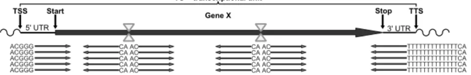
Figure 1: Schematic view of a transcriptional unit. RsaI restriction sites are indicated by yellow triangles. Transcript fragments (red) are sequenced starting from restriction sites in either direction, downstream from the transcription start site (TSS) as well as upstream from the transcription termination site (TTS), resulting in different sequence prefixes (GGG, CA, poly-T).
tools exists for that task, such as SOAP2 [LYL + 09], MAQ [LRD08], VMatch [Kur03], RazerS [WER + 09], and Bowtie [LTPS09]. Some pro- grams are able to map reads covering splice junctions (TopHat [TPS09], QPALMA [DBOSR08]), others can map reads against several genomes at once, such as GenomeMapper [SHO + 09]. Secondly, though more and more reference genomes are made available, the vast majority of organisms remain unsequenced and thus beyond the scope of RNA-seq studies.
Here we present Passage [H¨u09], extending the idea of SAGE to cre- ate a new efficient method for transcriptome studies in the absence of a reference genome sequence. It makes use of a newly established ex- perimental protocol resulting in reads originating only from well-defined genomic positions. Passage clusters these reads very efficiently to com- pute expression levels. Comparative studies can also be performed easily based on our method.
2 Material and Methods
Sample Preparation Purified mRNA is incubated with anchored Oligo (dT 13 ) and modified Smart (dG 3 ) oligonucleotides. These primers contain RsaI restriction sites. Reverse transcription is performed to obtain cDNA which is then amplified using long-distance PCR. After purification steps, the cDNA is cut into transcript fragments using the restriction enzyme RsaI. This step replaces the fragmentation step (e.g. by sonication) that is usually performed in RNA-seq protocols. Sequencing adapters are ligated to the fragments, and the fragments are analyzed by deep-sequencing.
The universal primer site can be used for different sequencing techniques
such as GS FLX TM (Roche Diagnostics/454) and the Genome Analyzer TM
(Illumina). Barcode sequences can be included in the adapters to allow
parallel sequencing of several samples. The resulting reads start with the
A C
G T C A
G T C
A A C T G
G T C
A A C T G
- Cluster 2 Read count: 1452 ACAAAAAAAAAAAAAC
>Read 73625615
>Read 23741928
>Read 29382541 ...
- Cluster 1 Read count: 345 ACAAAAAAAAAAAAAA
>Read 73625615
>Read 23741928
>Read 29382541 ...
- Cluster (n-1) Read count: 13 ACGGGGGGGGGGGT
>Read 73625615
>Read 23741928
>Read 29382541 ...
- Cluster n Read count: 57 ACGGGGGGGGGGGG
>Read 12536491
>Read 92846371
>Read 38274519 ...
FASTA
>Read 00000001 ACGGGTACAGAGTAGAGTC
>Read 00000002 ACGACTGAGCTTATGCTAT
>Read 00000003 ACGATGAGCTAGCATATCG
HASHTABLE[AAGTAA]Cluster 2536 Cluster 62543 Cluster 12837 Cluster 19927 [AGCAAT]
Cluster 42938 Cluster 13023 Cluster 19482
HASHTABLE[ACAAAA]Cluster 13627 Cluster 45832 Cluster 29384 [ACAAAT]
Cluster 31992 Cluster 18372 Cluster 59012
Cluster 39283 HASHTABLE[ACGATA]Cluster 39182 Cluster 31766 Cluster 33212 Cluster 81772 Cluster 46554 Cluster 48832 Cluster 415 [GCTAGC]
CLUSTER
- Cluster 1 Read count: 345 ACAAAAAAAAAAAAAAAA
>Read 73625615
>Read 23741928
>Read 29382541 ...- Cluster 2 Read count: 1452 ACAAAAAAAAAAAAAAAC
>Read 73625615
>Read 23741928
>Read 29382541 ...
Presorting Exact clustering
Hashing
Mismatch resolution
Figure 2: Passage workflow: Reads for one sample (after optional presorting) are used to build a trie, resulting in a clustering of perfectly matching sequences.
The reads’ sequences are split into three parts and a hash map is built for each such part. These hash maps are used in the mismatch resolution step to cluster all reads with at most two mismatches, resulting in the final clustering output.
optional barcode, followed by a prefix and the genomic sequence. Three types of fragments can be distinguished by their prefixes: 5’ UTR frag- ments start with ACGGG, 3’ UTR fragments with ACT 13 , and internal frag- ments with the restriction sequence AC (see figure 1). This protocol is adapted from [LRR + 10] describing a 3’-fingerprint analyzed on a 2-D gel electrophoresis system to next-generation sequencing transcriptomics.
Cluster algorithm Our read clustering algorithm, Passage, employs a three-step process. Starting from a fasta file containing read sequences, this involves presorting, exact clustering and mismatch resolution. The result is a file containing the number of reads contained in each cluster, the cluster’s consensus sequence, the IDs of the reads, and a normalized expression estimate (reads per million reads). Result files from multiple samples can be joined into a tabular file containing one column per sam- ple and one row per cluster, which can be analyzed with any standard microarray analysis software.
Presorting Reads are sequenced either from the 3’, the 5’ or the in-
terior region of a transcriptional unit. This is reflected in different read
prefixes (see figure 1). Differentiating the reads by these prefixes is not
only useful for reducing computational costs, but rather to allocate the
reads to the different parts of a transcriptional unit. With the addition
of barcode sequences, different samples can be analysed in the same se-
quencing run, adding another common prefix for all reads of that sample.
During presorting, reads are sorted according to their barcode (to distin- guish different samples) and their prefix.
Exact clustering Based on the presorting result, each prefix is pro- cessed as follows. A trie of read sequences is generated such that reads are assigned to a common leaf if their sequences are identical. Since we know that reads either overlap by 100% or not at all, this effectively clusters all reads deriving from the same transcript fragment. Reads are placed into the tree by matching their bases one by one to the corresponding tree path until either a leaf is reached (and the read sequence is completely matched) or a new branch has to be created to accomodate the read’s sequence. The result of the tree building step is a list of clusters, each cluster containing identical reads.
Mismatch resolution No current sequencing technology is error-free, thus we can not expect all reads from the same locus to be identical. In order to resolve this, we include a mismatch resolution step in our clus- tering algorithm. If k mismatches should be allowed, the minimal perfect match length results from equidistant distribution of these mismatches over the clusters’ sequences. Thus we partition the clusters’ sequences into k + 1 parts and create k + 1 hash maps. Clusters are placed into these hash maps according to the parts of their sequences. Thus, two clusters differing by at most k mismatches will be found in the same hash bucket in at least one of the hash maps. To ensure similar load factors in the presence of long common sequence prefixes, the first sequence part is slightly longer.
Clusters of identical reads are processed according to their size, starting with the largest cluster (in terms of the number of reads contained). From each hash map, candidate clusters are selected for merging. Ungapped alignments are computed and clusters are merged if their distance is at most k mismatches. Merged clusters are removed from all hash maps and the process is repeated until all clusters have been processed. Analysis showed that usually there is one very large and several smaller clusters for a given locus, and that the reads in the large cluster accurately represent the true genomic sequence. Thus we use the largest cluster’s sequence as the consensus sequence for the joined cluster.
3 Results
We illustrate our method using the two closely related yeast species Can-
dida albicans and Candida dubliniensis. Both are facultative pathogens,
100pg 1µg Dataset 1, 40bp C. albicans Y, 30 ◦ 4.1 † 4.6
· YF, 37 ◦ 3.7 5.1
C. dubliniensis · HF, 37 ◦ 4.9 4.8
YF, 37 ◦ 4.2 4.7
Dataset 2, 76bp C. dubliniensis · HF, 37 ◦ 7.6 / 7.6 ∗3.8 / 5.6 YF, 37 ◦ 4.4 / 5.5 ∗6.1 / 8.6 Table 1: Conditions and number of reads (millions) sequenced for the two datasets. Y, yeast extract peptone dextrose, is a complete medium for yeast growth. F, fetal calf serum (10%). H, H
2O. The amount of total RNA used for sequencing was either 100pg or 1µg. The second dataset contains replicate sequencings. Hyphae-inducing conditions are marked with (·). Data used for comparison with other tools is indicated with (†), those used for validation using microarrays are marked with (∗).
C. albicans is of higher clinical importance as the most common agent causing candidosis. Both species have a genome size of about 14Mb orga- nized in eight chromosomes and roughly the same number of genes (6185 in C. albicans, 5983 in C. dubliniensis). Cultures were grown under differ- ent conditions to study the induction of yeast or hyphae cell proliferation.
RNA-seq data was generated from different amounts of total RNA and different read lengths (see table 1). In total, we analyzed 16 RNA-seq runs, using Passage with a maximum of two mismatches.
To assess the robustness of the protocol, we compared the two sequenc- ings for each sample in dataset 1 by mapping the reads to all annotated genes (using Bowtie with up to two mismatches). More than 80% of the annotated genes found in the 100pg sample were also found in the 1µg sample, with the total number of transcripts being about twice as high in the 1µg samples (mean 4344 vs. 2247).
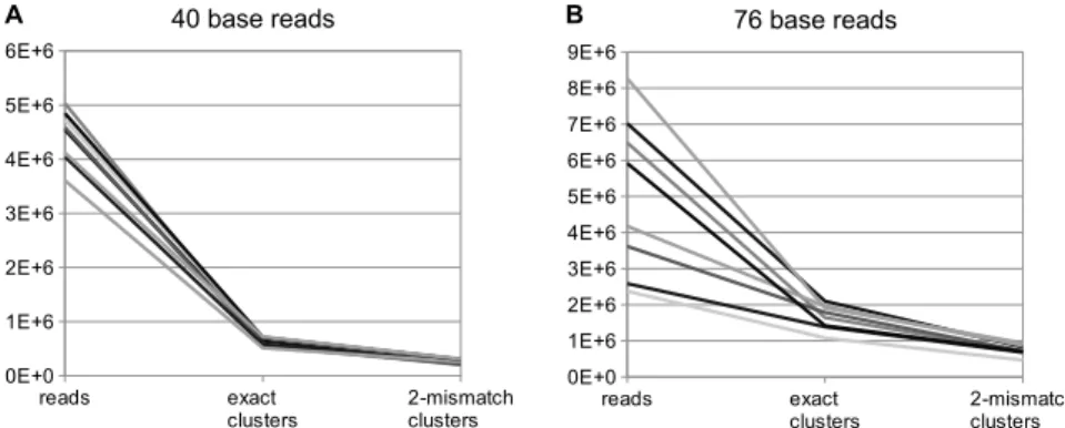
Data volume reduction Both clustering steps significantly reduce data volume (see figure 3). The efficiency of data reduction depends on the quality of the sequencing process. Fewer mismatches allow more reads to be clustered to their correct cluster and thus increase the reduction factor.
In our studies using 16 different datasets (8 with 40-mer reads, 8 with 76- mer reads), exact clustering reduced data volume by about 84% (factor 6.1). Mismatch resolution results in a further reduction by about 58%
(factor 2.4), resulting in a total reduction of about 93%. The reduction
during perfect clustering can be seen as the result of summarizing the
76 base reads 40 base reads
A B
reads exact
clusters 2-mismatch clusters 0E+0
1E+6 2E+6 3E+6 4E+6 5E+6 6E+6
reads exact
clusters 2-mismatch clusters 0E+0
1E+6 2E+6 3E+6 4E+6 5E+6 6E+6 7E+6 8E+6 9E+6
Figure 3: Reduction in data volume (number of reads resp. clusters) achieved by exact clustering and mismatch resolution. 16 datasets were analysed, eight of them with reads of length 40, eight with length 76. Longer reads (B) result in less reduction than shorter reads (A) due to higher error rates.
transcription strength (which varies between conditions) to the number of uniquely sequenced transcripts (which is expected to be more similar for all conditions). During the mismatch resolution step, a reduction is achieved by correcting for the error rate inherent in the sequencing technology, which should also be similar for all experiments.
Runtime analysis Presorting is important to reduce runtime and memory consumption and can be accomplished in O(n) where n is the number of input reads. Exact clustering can also be done in O(n). The time complexity of the mismatch resolution step depends on the average size of the hash buckets and the initial size of the cluster list: If c exact clusters are hashed randomly into buckets, let the average bucket size be . Merging the clusters can then be done in O( c · 2 ). In the worst case, all clusters are hashed into one bucket, yielding = c and O(c 2 ) runtime.
The optimal case would be = 1, yielding O(c) runtime.
For real data, we see very small values for : We found = 2.5 for reads of length 76 and = 4 for reads of length 40. Thus, for the average case can be considered constant which results in a runtime of O(c) (see figure 4A).
Even in cases where a large number of clusters are collected in one hash bucket, we observe runtime linear with respect to the sum of sizes of the largest buckets in each hash map (see figure 4B). As c is bounded by the number of reads, n, overall average runtime is O(n).
Comparison to other tools Passage was written to cluster short
reads and to use the size of the clusters as a measure of transcription.
A
0 100 200 300 400 500 600 700 800 900 1000
3E+5 8E+5 1E+6 2E+6 2E+6
Time[sec]
Exact clusters
B
0 500 1000 1500 2000 2500
25000 45000 65000 85000 105000
Time[sec]
Sum of largest hash buckets


![Figure 2: Toy example of a bipartite graph (a) from [LWZY06], with its backbone network and fuzzy clusters (b)](https://thumb-eu.123doks.com/thumbv2/1library_info/3946934.1534671/36.684.113.586.104.237/figure-example-bipartite-graph-lwzy-backbone-network-clusters.webp)