TheBelleCollaboration Testofleptonflavoruniversalityandsearchforleptonflavorviolationin B → Kℓℓ decays

arXiv:1908.01848v3 [hep-ex] 22 Apr 2021

Published as JHEP 03 (2021) 105

Belle Preprint 2020-11 KEK Preprint 2020-12

Test of lepton flavor universality and search for lepton flavor violation in B → Kℓℓ decays

The Belle Collaboration

S. Choudhury,

S. Sandilya,

K. Trabelsi,

A. Giri,

H. Aihara,

S. Al Said,

D. M. Asner,

H. Atmacan,

V. Aulchenko,

T. Aushev,

R. Ayad,

V. Babu,

S. Bahinipati,

P. Behera,

C. Beleño,

K. Belous,

J. Bennett,

F. Bernlochner,

M. Bessner,

V. Bhardwaj,

T. Bilka,

J. Biswal,

G. Bonvicini,

A. Bozek,

M. Bračko,

T. E. Browder,

M. Campajola,

D. Červenkov,

M.-C. Chang,

P. Chang,

V. Chekelian,

A. Chen,

B. G. Cheon,

K. Chilikin,

K. Cho,

S.-K. Choi,

Y. Choi,

D. Cinabro,

S. Cunliffe,

N. Dash,

G. De Nardo,

R. Dhamija,

F. Di Capua,

J. Dingfelder,

Z. Doležal,

T. V. Dong,

D. Dossett,

S. Dubey,

S. Eidelman,

D. Epifanov,

T. Ferber,

D. Ferlewicz,

B. G. Fulsom,

R. Garg,

V. Gaur,

N. Gabyshev,

A. Garmash,

P. Goldenzweig,

B. Golob,

D. Greenwald,

C. Hadjivasiliou,

O. Hartbrich,

H. Hayashii,

M. T. Hedges,

M. Hernandez Villanueva,

T. Higuchi,

W.-S. Hou,

C.-L. Hsu,

T. Iijima,

K. Inami,

A. Ishikawa,

R. Itoh,

M. Iwasaki,

Y. Iwasaki,

W. W. Jacobs,

E.-J. Jang,

H. B. Jeon,

S. Jia,

Y. Jin,

C. W. Joo,

K. K. Joo,

J. Kahn,

A. B. Kaliyar,

K. H. Kang,

G. Karyan,

H. Kichimi,

C. Kiesling,

B. H. Kim,

D. Y. Kim,

K.-H. Kim,

K. T. Kim,

S. H. Kim,

Y.-K. Kim,

K. Kinoshita,

P. Kodyš,

S. Korpar,

D. Kotchetkov,

P. Križan,

R. Kroeger,

P. Krokovny,

T. Kuhr,

R. Kulasiri,

R. Kumar,

K. Kumara,

A. Kuzmin,

Y.-J. Kwon,

K. Lalwani,

S. C. Lee,

P. Lewis,

C. H. Li,

L. K. Li,

Y. B. Li,

L. Li Gioi,

J. Libby,

K. Lieret,

Z. Liptak ,

D. Liventsev,

T. Luo,

M. Masuda,

T. Matsuda,

D. Matvienko,

M. Merola,

K. Miyabayashi,

R. Mizuk,

G. B. Mohanty,

S. Mohanty,

T. J. Moon,

T. Mori,

I. Nakamura,

K. R. Nakamura,

M. Nakao,

Z. Natkaniec,

A. Natochii,

L. Nayak,

M. Nayak,

M. Niiyama,

N. K. Nisar,

S. Nishida,

K. Ogawa,

H. Ono,

Y. Onuki,

P. Oskin,

P. Pakhlov,

G. Pakhlova,

S. Pardi,

H. Park,

S.-H. Park,

S. Patra,

S. Paul,

T. K. Pedlar,

R. Pestotnik,

L. E. Piilonen,

T. Podobnik,

V. Popov,

E. Prencipe,

M. T. Prim,

A. Rabusov,

A. Rostomyan,

N. Rout,

M. Rozanska,

G. Russo,

D. Sahoo,

Y. Sakai,

L. Santelj,

T. Sanuki,

V. Savinov,

G. Schnell,

J. Schueler,

†

now at Hiroshima University.

C. Schwanda,

A. J. Schwartz,

Y. Seino,

K. Senyo,

M. E. Sevior,

M. Shapkin,

V. Shebalin,

J.-G. Shiu,

B. Shwartz,

F. Simon,

A. Sokolov,

E. Solovieva,

S. Stanič,

M. Starič,

Z. S. Stottler,

T. Sumiyoshi,

W. Sutcliffe,

M. Takizawa,

U. Tamponi,

K. Tanida,

F. Tenchini,

M. Uchida,

S. Uehara,

T. Uglov,

Y. Unno,

S. Uno,

P. Urquijo,

Y. Ushiroda,

R. Van Tonder,

G. Varner,

K. E. Varvell,

A. Vinokurova,

V. Vorobyev,

E. Waheed,

C. H. Wang,

E. Wang,

M.-Z. Wang,

P. Wang,

M. Watanabe,

S. Watanuki,

S. Wehle,

J. Wiechczynski,

E. Won,

X. Xu,

B. D. Yabsley,

W. Yan,

S. B. Yang,

H. Ye,

J. Yelton,

J. H. Yin,

C. Z. Yuan,

Y. Yusa,

Z. P. Zhang,

V. Zhilich,

V. Zhukova

1

University of the Basque Country UPV/EHU, 48080 Bilbao, Spain

2

University of Bonn, 53115 Bonn, Germany

3

Brookhaven National Laboratory, Upton, New York 11973, USA

4

Budker Institute of Nuclear Physics SB RAS, Novosibirsk 630090, Russian Federation

5

Faculty of Mathematics and Physics, Charles University, 121 16 Prague, The Czech Republic

6

Chonnam National University, Gwangju 61186, South Korea

7

University of Cincinnati, Cincinnati, OH 45221, USA

8

Deutsches Elektronen–Synchrotron, 22607 Hamburg, Germany

9

University of Florida, Gainesville, FL 32611, USA

10

Department of Physics, Fu Jen Catholic University, Taipei 24205, Taiwan

11

Key Laboratory of Nuclear Physics and Ion-beam Application (MOE) and Institute of Modern Physics, Fudan University, Shanghai 200443, PR China

12

II. Physikalisches Institut, Georg-August-Universität Göttingen, 37073 Göttingen, Germany

13

SOKENDAI (The Graduate University for Advanced Studies), Hayama 240-0193, Japan

14

Gyeongsang National University, Jinju 52828, South Korea

15

Department of Physics and Institute of Natural Sciences, Hanyang University, Seoul 04763, South Korea

16

University of Hawaii, Honolulu, HI 96822, USA

17

High Energy Accelerator Research Organization (KEK), Tsukuba 305-0801, Japan

18

J-PARC Branch, KEK Theory Center, High Energy Accelerator Research Organization (KEK), Tsukuba 305-0801, Japan

19

Higher School of Economics (HSE), Moscow 101000, Russian Federation

20

Forschungszentrum Jülich, 52425 Jülich, Germany

21

IKERBASQUE, Basque Foundation for Science, 48013 Bilbao, Spain

22

Indian Institute of Science Education and Research Mohali, SAS Nagar, 140306, India

23

Indian Institute of Technology Bhubaneswar, Satya Nagar 751007, India

24

Indian Institute of Technology Hyderabad, Telangana 502285, India

25

Indian Institute of Technology Madras, Chennai 600036, India

26

Indiana University, Bloomington, IN 47408, USA

27

Institute of High Energy Physics, Chinese Academy of Sciences, Beijing 100049, PR China

28

Institute for High Energy Physics, Protvino 142281, Russian Federation

29

Institute of High Energy Physics, Vienna 1050, Austria

30

INFN - Sezione di Napoli, 80126 Napoli, Italy

31

INFN - Sezione di Torino, 10125 Torino, Italy

32

Advanced Science Research Center, Japan Atomic Energy Agency, Naka 319-1195, Japan

33

J. Stefan Institute, 1000 Ljubljana, Slovenia

34

Institut für Experimentelle Teilchenphysik, Karlsruher Institut für Technologie, 76131 Karlsruhe, Germany

35

Kavli Institute for the Physics and Mathematics of the Universe (WPI), University of Tokyo, Kashiwa 277-8583, Japan

36

Kennesaw State University, Kennesaw GA 30144, USA

37

Department of Physics, Faculty of Science, King Abdulaziz University, Jeddah 21589, Saudi Ara- bia

38

Korea Institute of Science and Technology Information, Daejeon 34141, South Korea

39

Korea University, Seoul 02841, South Korea

40

Kyoto Sangyo University, Kyoto 603-8555, Japan

41

Kyoto University, Kyoto 606-8502, Japan

42

Kyungpook National University, Daegu 41566, South Korea

43

Université Paris-Saclay, CNRS/IN2P3, IJCLab, 91405 Orsay, France

44

P.N. Lebedev Physical Institute of the Russian Academy of Sciences, Moscow 119991, Russian Federation

45

Liaoning Normal University, Dalian 116029, China

46

Faculty of Mathematics and Physics, University of Ljubljana, 1000 Ljubljana, Slovenia

47

Ludwig Maximilians University, 80539 Munich, Germany

48

Luther College, Decorah, IA 52101, USA

49

Malaviya National Institute of Technology Jaipur, Jaipur 302017, India

50

University of Maribor, 2000 Maribor, Slovenia

51

Max-Planck-Institut für Physik, 80805 München, Germany

52

School of Physics, University of Melbourne, Victoria 3010, Australia

53

University of Mississippi, University, MS 38677, USA

54

University of Miyazaki, Miyazaki 889-2192, Japan

55

Moscow Physical Engineering Institute, Moscow 115409, Russian Federation

56

Graduate School of Science, Nagoya University, Nagoya 464-8602, Japan

57

Kobayashi-Maskawa Institute, Nagoya University, Nagoya 464-8602, Japan

58

Università di Napoli Federico II, 80126 Napoli, Italy

59

Nara Women’s University, Nara 630-8506, Japan

60

National Central University, Chung-li 32054, Taiwan

61

National United University, Miao Li 36003, Taiwan

62

Department of Physics, National Taiwan University, Taipei 10617, Taiwan

63

H. Niewodniczanski Institute of Nuclear Physics, Krakow 31-342, Poland

64

Nippon Dental University, Niigata 951-8580, Japan

65

Niigata University, Niigata 950-2181, Japan

66

University of Nova Gorica, 5000 Nova Gorica, Slovenia

67

Novosibirsk State University, Novosibirsk 630090, Russian Federation

68

Osaka City University, Osaka 558-8585, Japan

69

Osaka University, Osaka 565-0871, Japan

70

Pacific Northwest National Laboratory, Richland, WA 99352, USA

71

Panjab University, Chandigarh 160014, India

72

Peking University, Beijing 100871, PR China

73

University of Pittsburgh, Pittsburgh, PA 15260, USA

74

Punjab Agricultural University, Ludhiana 141004, India

75

Research Center for Nuclear Physics, Osaka University, Osaka 567-0047, Japan

76

Meson Science Laboratory, Cluster for Pioneering Research, RIKEN, Saitama 351-0198, Japan

77

Theoretical Research Division, Nishina Center, RIKEN, Saitama 351-0198, Japan

78

Department of Modern Physics and State Key Laboratory of Particle Detection and Electronics, University of Science and Technology of China, Hefei 230026, PR China

79

Seoul National University, Seoul 08826, South Korea

80

Showa Pharmaceutical University, Tokyo 194-8543, Japan

81

Soochow University, Suzhou 215006, China

82

Soongsil University, Seoul 06978, South Korea

83

Sungkyunkwan University, Suwon 16419, South Korea

84

School of Physics, University of Sydney, New South Wales 2006, Australia

85

Department of Physics, Faculty of Science, University of Tabuk, Tabuk 71451, Saudi Arabia

86

Tata Institute of Fundamental Research, Mumbai 400005, India

87

Department of Physics, Technische Universität München, 85748 Garching, Germany

88

School of Physics and Astronomy, Tel Aviv University, Tel Aviv 69978, Israel

89

Toho University, Funabashi 274-8510, Japan

90

Department of Physics, Tohoku University, Sendai 980-8578, Japan

91

Earthquake Research Institute, University of Tokyo, Tokyo 113-0032, Japan

92

Department of Physics, University of Tokyo, Tokyo 113-0033, Japan

93

Tokyo Institute of Technology, Tokyo 152-8550, Japan

94

Tokyo Metropolitan University, Tokyo 192-0397, Japan

95

Utkal University, Bhubaneswar 751004, India

96

Virginia Polytechnic Institute and State University, Blacksburg, VA 24061, USA

97

Wayne State University, Detroit, MI 48202, USA

98

Yamagata University, Yamagata 990-8560, Japan

99

Yonsei University, Seoul 03722, South Korea

Abstract: We present measurements of the branching fractions for the decays B →

Kµ

µ

and B → Ke

e

, and their ratio (R

), using a data sample of 711 fb

that

contains 772 × 10

B B ¯ events. The data were collected at the Υ(4S) resonance with the

Belle detector at the KEKB asymmetric-energy e

e

collider. The ratio R

is measured

in five bins of dilepton invariant-mass-squared (q

): q

∈ (0.1, 4.0), (4.00, 8.12), (1.0, 6.0),

(10.2, 12.8) and (> 14.18) GeV

/c

, along with the whole q

region. The R

value for

q

∈ (1.0, 6.0) GeV

/c

is 1.03

± 0.01. The first and second uncertainties listed are

statistical and systematic, respectively. All results for R

are consistent with Standard

Model predictions. We also measure CP-averaged isospin asymmetries in the same q

bins. The results are consistent with a null asymmetry, with the largest difference of 2.6

standard deviations occurring for the q

∈ (1.0, 6.0) GeV

/c

bin in the mode with muon

final states. The measured differential branching fractions, dB/dq

, are consistent with

theoretical predictions for charged B decays, while the corresponding values are below

the expectations for neutral B decays. We have also searched for lepton-flavor-violating

B → Kµ

e

decays and set 90% confidence-level upper limits on the branching fraction in

the range of 10

for B

→ K

µ

e

, and B

→ K

µ

e

modes.

Contents

1 Introduction 1

2 Data samples and Belle detector 2

3 Analysis Overview 2

4 Results 6

5 Systematic uncertainties 14

6 Summary 15

7 Acknowledgments 16

1 Introduction

The decays B → Kℓ

ℓ

(ℓ = e, µ), mediated by the b → sℓ

ℓ

quark-level transition, constitute a flavor-changing neutral current process. Such processes are forbidden at tree level in the Standard Model (SM) but can proceed via suppressed loop-level diagrams, and they are therefore sensitive to particles predicted in a number of new physics models [1, 2].

A robust observable [3] to test the SM prediction is the lepton-flavor-universality (LFU) ratio,

R

= R

dq²

[B → Hµ

µ

]dq

R

dq²

[B → He

e

]dq

, (1.1) where H is a K or K

meson and the decay rate Γ is integrated over a range of the dilepton invariant mass squared, q

≡ M

(ℓ

ℓ

). For R

, recently LHCb [4] reported hints of deviations from SM expectations, while Belle [5] results are consistent with the SM with relatively larger uncertainties. LHCb also measured R

[6], reporting a difference of about 2.5 standard deviations (σ) from the SM prediction in the q

∈ (1.1, 6.0) GeV

/c

bin. A previous measurement of the same quantity was performed by Belle [7] in the whole q

range with a data sample of 657 × 10

B B ¯ events. The result presented here is obtained from a multidimensional fit performed on the full Belle data sample of 772 ×10

B B ¯ events, and supersedes our previous result [7].

Another theoretically robust observable [8], where the dominant form-factor-related uncertainties also cancel, is the CP -averaged isospin asymmetry, representing the difference in partial widths:

A

= (τ

/τ

)B(B

→ K

ℓ

ℓ

) − B(B

→ K

ℓ

ℓ

)

(τ

/τ

)B(B

→ K

ℓ

ℓ

) + B(B

→ K

ℓ

ℓ

) , (1.2)

where τ

/τ

= 1.078 ± 0.004 is the lifetime ratio of B

to B

[9]. The f

/f

= 1.058± 0.024 [10] is the relative production fraction of charged (f

) and neutral B mesons (f

) at B factories. The A

value is expected to be close to zero in the SM [11]. Earlier, BaBar [12] and Belle [7] reported A

to be significantly below zero, especially in the q

region below the J/ψ resonance, while LHCb [13] reported results consistent with SM predictions.

In many theoretical models, lepton flavor violation (LFV) accompanies LFU viola- tion [14]. With neutrino mixing, LFV is only possible at rates far below the current ex- perimental sensitivity. In case of signal, this will signify physics beyond SM [15]. The LFV in B decays can be studied via B → Kµ

e

. The most stringent upper limits on B

→ K

µ

e

and B

→ K

µ

e

set by LHCb [16] are 6.4 × 10

and 7.0 × 10

at 90% confidence level (CL). Prior to that, B

→ K

µ

e

decays were searched for by BaBar [17], which set a 90% CL upper limit on the branching fraction of 2.7 × 10

.

In this paper, we report a measurement of the decay branching fractions of B → Kℓ

ℓ

, R

and A

in the whole q

range as well as in five q

bins [(0.1, 4.0), (4.00, 8.12), (1.0, 6.0), (10.2, 12.8) and (> 14.18)] GeV

/c

. We also search for B → Kµ

e

decays using the full Belle data sample.

2 Data samples and Belle detector

This analysis uses a 711 fb

data sample containing (772 ± 11) × 10

B B ¯ events, collected at the Υ(4S) resonance by the Belle experiment at the KEKB e

e

collider [18]. An 89 fb

data sample recorded 60 MeV below the Υ(4S) peak (off-resonance) is used to estimate the background contribution from e

e

→ q q ¯ (q = u, d, s, c) continuum events.

The Belle detector [19] is a large-solid-angle magnetic spectrometer composed of a silicon vertex detector (SVD), a 50-layer central drift chamber (CDC), an array of aerogel threshold Cherenkov counters (ACC), a barrel-like arrangement of time-of-flight scintillation counters (TOF), and an electromagnetic calorimeter (ECL) comprising CsI(Tl) crystals.

All these subdetectors are located inside a superconducting solenoid coil that provides a 1.5 T magnetic field. An iron flux-return yoke placed outside the coil is instrumented with resistive plate chambers (KLM) to detect K

mesons and muons. Two inner detector configurations were used: a 2.0 cm radius beam pipe and a three-layer SVD for the first sample of 140 fb

; and a 1.5 cm radius beam pipe, a four-layer SVD, and a small-cell inner CDC for the remaining 571 fb

[20].

To study properties of signal events and optimize selection criteria, we use samples of Monte Carlo (MC) simulated events. The B → Kℓ

ℓ

modes are generated with the EvtGen package [21] based on a model described in Ref. [22], while LFV modes are generated with a phase-space model. The PHOTOS [23] package is used to incorporate final-state radiation. The detector response is simulated with GEANT3 [24].

3 Analysis Overview

We reconstruct B → Kℓ

ℓ

(K = K

, K

) [25] decays by selecting charged particles that originate from the vicinity of the e

e

interaction point (IP), except for those originating

– 2 –

from K

decays. We require impact parameters less than 1.0 cm in the transverse plane and less than 4.0 cm along the z axis (parallel to the e

beam). To reduce backgrounds from low-momentum particles, we require that tracks have a minimum transverse momentum of 100 MeV /c .

From the list of selected tracks, we identify K

candidates using a likelihood ratio R

= L

/(L

+ L

), where L

and L

are the likelihoods for charged kaons and pions, respectively, calculated based on the number of photoelectrons in the ACC, the specific ionization in the CDC, and the time of flight as determined from the TOF. We select kaons by requiring R

> 0.6, which has a kaon identification efficiency of 92%

and a pion misidentification rate of 7%. For the neutral B decay, candidate K

mesons are reconstructed by combining two oppositely charged tracks (assumed to be pions) with an invariant mass between 487 and 508 MeV /c

; this corresponds to a 3σ window around the nominal K

mass [9]. Such candidates are further identified with a neural network (NN). The variables used for this NN are: the K

momentum; the distance along the z axis between the two track helices at their closest approach; the flight length in the transverse plane; the angle between the K

momentum and the vector joining the IP with the K

decay vertex; the angle between the pion momentum and the laboratory-frame direction in the K

rest frame; the distances-of-closest-approach in the transverse plane between the IP and the two pion helices; and the number of hits in the CDC; and the presence or absence of hits in the SVD for each pion track.

Muon candidates are identified based on information from the KLM. We require that candidates have a momentum greater than 0.8 GeV /c (enabling them to reach the KLM subdetector), and a penetration depth and degree of transverse scattering consistent with those of a muon [26]. The latter information is used to calculate a normalized muon likelihood R

, and we require R

> 0.9. For this requirement, the average muon detection efficiency is 89%, with a pion misidentification rate of 1.5% [27].

Electron candidates are required to have a momentum greater than 0.5 GeV /c and are identified using the ratio of calorimetric cluster energy to the CDC track momentum; the shower shape in the ECL; the matching of the track with the ECL cluster; the specific ionization in the CDC; and the number of photoelectrons in the ACC. This information is used to calculate a normalized electron likelihood R

, and we require R

> 0.9. This requirement has an efficiency of 92% and a pion misidentification rate below 1% [28]. To recover energy loss due to possible bremsstrahlung, we search for photons inside a cone of radius 50 mrad centered around the electron direction. For each photon found within the cone, its four-momentum is added to that of the initial electron.

Charged (neutral) B candidates are reconstructed by combining K

(K

) with suitable µ

or e

candidates. To distinguish signal from background events, two kinematic variables are used: the beam-energy-constrained mass M

= p

(E

/c

)

− (p

/c)

, and the

energy difference ∆E = E

− E

, where E

is the beam energy, and E

and p

are the energy and momentum, respectively, of the B candidate. All these quantities are

calculated in the e

e

center-of-mass (CM) frame. For signal events, the ∆E distribution

peaks at zero, and the M

distribution peaks near the B mass. We retain candidates

satisfying the requirements −0.10 < ∆E < 0.25 GeV and M

> 5.2 GeV /c

.

With the above selection criteria applied, about 2% of signal MC events are found to have more than one B candidate. For these events, we retain the candidate with smallest χ

value resulting from a vertex fit of the B daughter particles. From MC simulation, this criterion is found to select the correct signal candidate 78-85% of the time, depending on the decay mode. The decays B → J/ψ(→ ℓ

ℓ

)K and B → ψ(2S)(→ ℓ

ℓ

)K, used later as control samples, are suppressed in the signal selection via a set of vetoes 8.75 < q

<

10.2 GeV

/c

and 13.0 < q

< 14.0 GeV

/c

with the dimuon; 8.12 < q

< 10.2 GeV

/c

and 12.8 < q

< 14.0 GeV

/c

with the dielectron final states for B → J/ψK and B → ψ(2S)K, respectively. An additional veto of the low q

region (< 0.05 GeV

/c

) is applied in the case of B → Ke

e

to suppress possible contaminations from γ

→ e

e

and π

→ γe

e

.

At this stage of the analysis, there is significant background from continuum processes and other B decays. As lighter quarks are produced with large kinetic energy, the former events tend to consist of two back-to-back jets of pions and kaons. In contrast, B B ¯ events are produced almost at rest in the CM frame, resulting in more spherically distributed daughter particles. We thus distinguish B B ¯ events from q q ¯ background based on event topology.

Background arising from B decays has typically two uncorrelated leptons in the final state. Such background falls into three categories: (a) both B and B ¯ decay semileptonically;

(b) a B → D ¯

Xℓ

ν decay is followed by D ¯

→ Xℓ

ν ¯ ; and (c) hadronic B decays where one or more daughter particles are misidentified as leptons. To suppress continuum as well as B B ¯ background, we use an NN trained with the following input variables:

1. A likelihood ratio constructed from a set of modified Fox-Wolfram moments [29, 30].

2. The angle θ

between the B flight direction and the z axis in the CM frame (for B B ¯ events, dN/d cos θ

∝ 1 − cos

θ

, whereas for continuum events, dN/d cos θ

≈

constant, where N is the number of events).

3. The angle θ

between the thrust axes calculated from final-state particles for the candidate B and for the rest of the event in the CM frame. (The thrust axis is the direction that maximizes the sum of the longitudinal momenta of the considered particles). For signal events, the cos θ

distribution is flat, whereas for continuum events it peaks near ±1.

4. Flavor-tagging information from the tag-side (recoiling) B decay. The flavor-tagging algorithm [31] outputs two variables: the flavor q of the tag-side B, and the tag qual- ity r. The latter ranges from zero for no flavor information to one for an unambiguous flavor assignment.

5. The confidence level of the B vertex fitted from all daughter particles.

6. The separation in z between the signal B decay vertex and that of the other B in the event.

7. The separation between the two leptons along the z-axis divided by the quadratic sum of uncertainties in the z-intercepts of the tracks.

– 4 –

8. The sum of the ECL energy of tracks and clusters not associated with the signal B decay.

9. A set of variables developed by CLEO [32] that characterize the momentum flow into concentric areas around the thrust axis of a reconstructed B candidate.

The NN outputs a single variable O, for which larger values correspond to more signal- like events. To facilitate modeling of the distribution of O with an analytic function, we require O > −0.6 (= O

) and transform O to a new variable:

O

= log

O − O

O

− O

,

where O

is the upper boundary of O. The criterion on O

reduces the background events by more than 75%, with a signal loss of only 4-5%.

We study the remaining background events using MC simulation for individual modes, with special attention paid to those that can mimic signal decays. Candidates arising from B

→ J/ψ(→ ℓ

ℓ

)K

populate towards the negative side in ∆E and are sup- pressed with the requirement ∆E > −0.1 GeV. The decay B

→ D ¯

(→ K

π

)π

mimics B

→ K

µ

µ

when both pions are mis-identified as muons; to suppress this back- ground, we apply a veto on the invariant mass of the K

and µ

candidates: M[K

µ

] ∈ / (1.85, 1.88) GeV /c

. The contribution from other B → charm decays is negligible. Events originating from the decays B

→ J/ψ(→ µ

µ

)K

, in which one of the muons is misidentified as a kaon and vice versa, contribute as a peaking background to B

→ K

µ

µ

. Such events are suppressed by applying a veto on the invariant mass M [K

µ

] ∈ / (3.06, 3.13) GeV /c

.

For the LFV modes, the background coming from B

→ J/ψ(→ e

e

)K

because of

misidentification and swapping between particles is removed by invariant mass vetoes. For

the B

→ K

µ

e

mode, two vetoes are applied: (a) the electron is misidentified as kaon

and kaon as muon, and thus the veto on the kaon-electron invariant mass is M[K

e

] ∈ /

(2.95, 3.11) GeV /c

; and (b) the electron is misidentified as a muon, and thus the muon-

electron mass veto is M [µ

e

] ∈ / (3.02, 3.12) GeV /c

. For the B

→ K

µ

e

channel, only

the latter background is found and removed using M[µ

e

] ∈ / (3.02, 3.12) GeV /c

. A small

contribution from B

→ D ¯

(K

π

)π

for these LFV modes, due to misidentification of

pions as leptons, is removed by requiring M [K

µ

] ∈ / (1.85, 1.88) GeV /c

. For the B

→

K

µ

e

mode, a background contribution from B

→ J/ψ(→ e

e

)K

, where an electron

is misrecontructed as a muon, is suppressed by requiring M[µ

e

] ∈ / (3.04, 3.12) GeV /c

.

When calculating invariant masses for these vetoes, the mass hypothesis for the misidentified

particle is used. There is a small background from B → Kπ

π

decays in the B

→

K

µ

µ

(1.37 ± 0.03 events), B

→ K

µ

µ

(0.17 ± 0.01 events), B

→ K

µ

e

(0.16 ± 0.03 events), B

→ K

µ

e

(0.14 ± 0.03 events), and B

→ K

µ

e

(0.14 ± 0.02

events) samples. This background is negligible in the B

→ K

e

e

and B

→ K

e

e

samples. The mentioned yields of peaking charmless B backgrounds are estimated by

considering all known intermediate resonances. To avoid biasing our results, all selection

criteria are determined in a “blind” manner, i.e., they are finalized before looking at data events in the signal region.

We determine the signal yields by performing a three-dimensional unbinned extended maximum-likelihood fit to the M

, ∆E, and O

distributions in different q

bins. The fits are performed for each mode separately. The probability density functions (PDFs) used to model signal decays are as follows: for M

we use a Gaussian, for ∆E the sum of a Gaussian and a Crystal Ball function [33], and for O

the sum of a Gaussian and an asym- metric Gaussian with a common mean. All signal shape parameters are obtained from MC simulation. To account for small differences observed between data and MC simulations, we introduce an offset in the mean positions and scaling factors for the widths. The val- ues of these parameters are obtained from fitting the control sample B → J/ψ(→ ℓ

ℓ

)K decays and kept fixed. The PDFs used for charmless B → Kπ

π

peaking background is the same as that of the signal PDFs, with the fixed number of peaking events. The shapes of the M

, ∆E, and O

distributions for background arising from B decays are parameterized with an ARGUS function [34], an exponential, and a Gaussian function, re- spectively. Similarly, the continuum background is modeled using an ARGUS, a first-order polynomial, and a Gaussian function. The shapes of B B ¯ and continuum backgrounds are very similar in two of the fit variables, making it difficult to simultaneously float the yields of both backgrounds. Hence, the continuum yields are obtained for each mode from the off-resonance data sample and fixed in the fit. These yields are consistent with those of the high-statistics off-resonance MC sample. The B B ¯ yields are floated in the fit.

4 Results

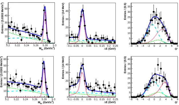
The results of the fit projected into a signal-enhanced region for M

[|∆E| < 0.05 GeV and O

∈ (1.0, 8.0)], ∆E [M

∈ (5.27, 5.29) GeV /c

and O

∈ (1.0, 8.0)] and O

[M

∈ (5.27, 5.29) GeV /c

and |∆E| < 0.05 GeV] distributions in the data sample are shown in Figs. 1 and 2 for B

→ K

ℓ

ℓ

and B

→ K

ℓ

ℓ

, respectively. These distributions correspond to the whole q

; q

∈ [(0.1, 8.75)(10.2, 13)(> 14.18)] GeV

/c

with muon and q

∈ [(0.1, 8.12)(10.2, 12.8)(> 14.18)] GeV

/c

with electron, in the final states.

There are 137 ± 14 and 138 ± 15 signal events for the decays B

→ K

µ

µ

and B

→ K

e

e

, respectively, whereas the yields for the decays B

→ K

µ

µ

and B

→ K

e

e

are 27.3

and 21.8

events, respectively. The fit is also performed in the aforementioned five q

bins [(0.1, 4.0), (4.00, 8.12), (1.0, 6.0), (10.2, 12.8), and (> 14.18)] GeV

/c

including the (1.0, 6.0) GeV

/c

bin, where LHCb reports a possible de- viation in R

, and R

and A

values are calculated from Eqs. (1.1) and (1.2), respectively.

The results are listed in Table 1 and R

and A

are also shown in Figs. 3 and 4, respectively.

The differential branching fraction (dB/dq

) results are shown in Fig. 5. The branching fractions for the B

→ K

ℓ

ℓ

, and B

→ K

ℓ

ℓ

modes are (5.99

± 0.14) × 10

, and (3.51

± 0.10) × 10

, respectively for the whole q

range. The measurement is done for B

→ K

ℓ

ℓ

, but the branching fraction is quoted for B

→ K

ℓ

ℓ

, con- sidering a factor of 2. Figure 6 illustrates the fit for B → J/ψ(→ ℓ

ℓ

)K modes and the corresponding branching fractions obtained are listed in Table 2. These samples serve

– 6 –

5.2 5.22 5.24 5.26 5.28 5.3

2) (GeV/c Mbc

0 10 20 30 40 50 )2Entries / (3.0303 MeV/c

−0.1−0.05 0 0.05 0.1 0.15 0.2 0.25 E (GeV)

∆ 0

10 20 30 40

Entries / (14 MeV)

−8 −6 −4 −2 0 2 4 6 8 O’

0 5 10 15 20 25 30 35

Entries / (0.5)

5.2 5.22 5.24 5.26 5.28 5.3

2) (GeV/c Mbc

0 10 20 30 40 50 60 )2Entries / (3.0303 MeV/c

−0.1−0.05 0 0.05 0.1 0.15 0.2 0.25 E (GeV)

∆ 0

10 20 30 40

Entries / (14 MeV)

−8 −6 −4 −2 0 2 4 6 8 O’

0 5 10 15 20 25 30 35 40

Entries / (0.5)

Figure 1. Signal-enhanced M

(left), ∆E (middle), and O

(right) projections of three-dimensional unbinned extended maximum-likelihood fits to the data events that pass the selection criteria for B

→ K

µ

µ

(top), and B

→ K

e

e

(bottom). Points with error bars are the data; blue solid curves are the fitted results for the signal-plus-background hypothesis; red dashed curves denote the signal component; cyan long dashed, green dash-dotted, and black dashed curves represent continuum, B B ¯ background, and B → charmless decays, respectively.

as calibration modes for the PDF shapes used as well as to calibrate the efficiency of

O > O

requirement for possible difference between data and simulation. These are also

used to verify that there is no bias for some of the key observables. For example, we ob-

tain R

(J/ψ) = 0.994 ± 0.011 ± 0.010 and 0.993 ± 0.015 ± 0.010 for B

→ J/ψK

and

B → J/ψK

, respectively. Similarly, A

(B → J/ψK) is −0.002 ± 0.006 ± 0.014.

5.2 5.22 5.24 5.26 5.28 5.3

2) (GeV/c Mbc

0 5 10 15 )2Entries / (3.0303 MeV/c

−0.1−0.05 0 0.05 0.1 0.15 0.2 0.25 E (GeV)

∆ 0

5 10 15

Entries / (14 MeV)

−8 −6 −4 −2 0 2 4 6 8 O’

0 2 4 6 8 10 12 14

Entries / (0.5)

5.2 5.22 5.24 5.26 5.28 5.3

2) (GeV/c Mbc

0 5 10 15 )2Entries / (3.0303 MeV/c

−0.1−0.05 0 0.05 0.1 0.15 0.2 0.25 E (GeV)

∆ 0

2 4 6 8 10 12

Entries / (14 MeV)

−8 −6 −4 −2 0 2 4 6 8 O’

0 2 4 6 8 10 12

Entries / (0.5)

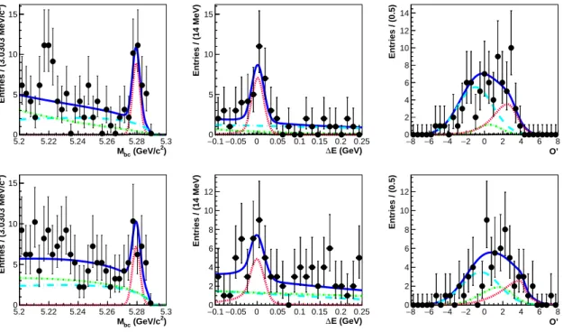
Figure 2. Signal-enhanced M

(left), ∆E (middle), and O

(right) projections of three-dimensional unbinned extended maximum-likelihood fits to the data events that pass the selection criteria for B

→ K

µ

µ

(top), and B

→ K

e

e

(bottom). The legends are the same as in Fig. 1.

– 8 –

Table 1. Results from the fits. The columns correspond to the q

bin size, decay mode, reconstruction efficiency, signal yield, branching fraction, lepton-flavor-separated and combined A

and R

.

q

B → mode ε N

B A

A

R

R

( GeV

/c

) (%) (10

) (individual) (combined) (individual) (combined)

(0.1,4.0)

K

µ

µ

20.4 28.4

1.76

± 0.04 A

(µµ) =

−0.22

± 0.01

R

=

1.01

± 0.02 K

µ

µ

14.7 6.8

0.62

± 0.02 −0.11

± 0.01 0.98

± 0.02

K

e

e

29.1 41.5

1.80

± 0.05 A

(ee) = R

S

= K

e

e

19.3 5.5

0.38

± 0.01 −0.35

± 0.01 1.62

± 0.02

(4.00,8.12)

K

µ

µ

29.0 28.4

1.24

± 0.03 A

(µµ) =

−0.09

± 0.01

R

=

0.85

± 0.01 K

µ

µ

21.0 4.2

0.27

± 0.01 −0.34

± 0.01 1.29

± 0.02

K

e

e

35.4 26.9

0.96

± 0.03 A

(ee) = R

S

= K

e

e

23.9 9.3

0.52

± 0.02 0.10

± 0.01 0.51

± 0.01

(1.0,6.0)

K

µ

µ

23.2 42.3

2.30

± 0.05 A

(µµ) =

−0.31

± 0.01

R

=

1.03

± 0.01 K

µ

µ

16.8 3.9

0.31

± 0.01 −0.53

± 0.02 1.39

± 0.02

K

e

e

31.7 41.7

1.66

± 0.04 A

(ee) = R

S

= K

e

e

21.1 8.9

0.56

± 0.02 −0.13

± 0.01 0.55

± 0.01

(10.2,12.8)

K

µ

µ

35.6 24.3

0.86

± 0.02 A

(µµ) =

−0.18

± 0.01

R

=

1.97

± 0.02 K

µ

µ

26.5 5.7

0.29

± 0.01 −0.14

± 0.01 1.96

± 0.02

K

e

e

40.3 14.0

0.44

± 0.01 A

(ee) = R

S

= K

e

e

26.5 1.1

0.06

± 0.01 −0.55

± 0.01 5.18

± 0.06

> 14.18

K

µ

µ

45.2 47.9

1.34

± 0.03 A

(µµ) =

−0.14

± 0.01

R

=

1.16

± 0.01 K

µ

µ

25.7 9.6

0.49

± 0.01 −0.08

± 0.01 1.13

± 0.01

K

e

e

46.2 43.2

1.18

± 0.03 A

(ee) = R

S

= K

e

e

24.9 5.9

0.32

± 0.01 −0.24

± 0.01 1.57

± 0.02

whole q

K

µ

µ

27.8 137.0

6.24

± 0.16 A

(µµ) =

−0.19

± 0.01

R

=

1.10

± 0.02 K

µ

µ

18.5 27.3

1.97

± 0.06 −0.16

± 0.01 1.08

± 0.02

K

e

e

30.3 138.0

5.75

± 0.15 A

(ee) = R

=

– 9 –

4

)

2

/c (GeV q

0 5 10 15 20

+K

R

0 0.2 0.4 0.6 0.8 1 1.2 1.4 1.6 1.8 2

4

)

2

/c (GeV q

0 5 10 15 20

K0

R

0 0.2 0.4 0.6 0.8 1 1.2 1.4 1.6 1.8 2

4 )

2 /c (GeV q 2

0 5 10 15 20

K R

0 0.2 0.4 0.6 0.8 1 1.2 1.4 1.6 1.8 2

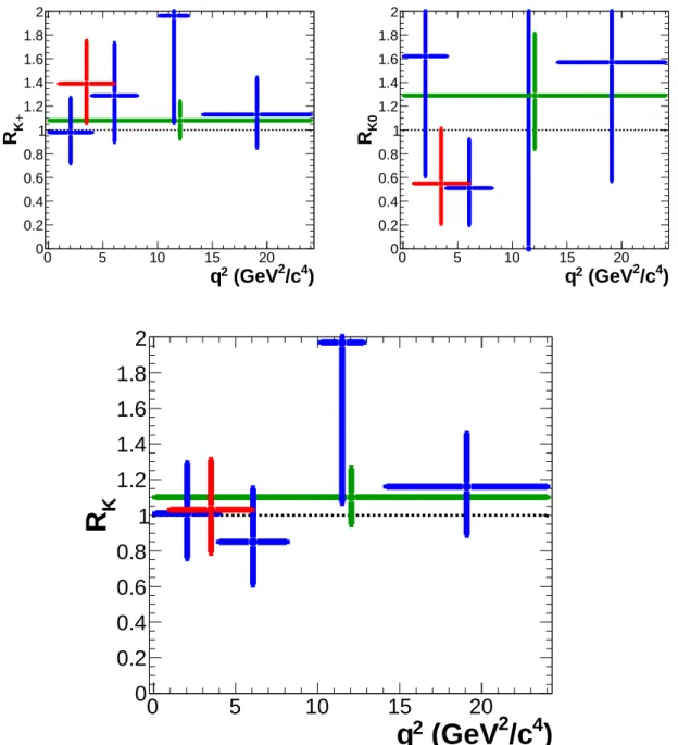
Figure 3. R

in bins of q

, for B

→ K

ℓ

ℓ

(top-left), B

→ K

ℓ

ℓ

(top-right), and both modes combined (bottom). The red marker represents the bin of 1.0 < q

< 6.0 GeV

/c

, and the blue markers are for 0.1 < q

< 4.0, 4.00 < q

< 8.12, 10.2 < q

< 12.8 and q

> 14.18 GeV

/c

bins. The green marker denotes the whole q

region excluding the charmonium resonances.

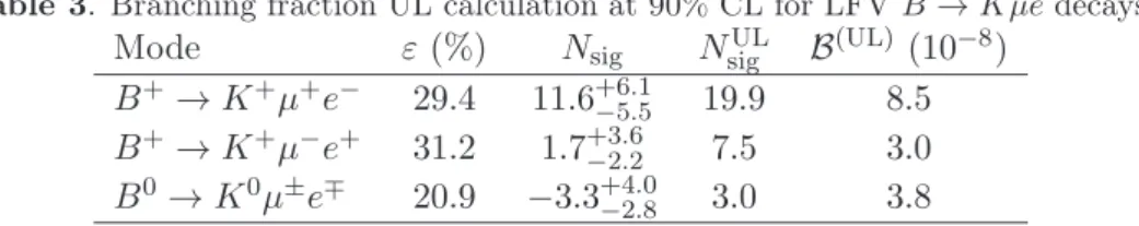
The signal yields for LFV decays are obtained by performing unbinned extended maximum- likelihood fits, similar to those for the B → Kℓ

ℓ

modes. The signal-enhanced projection plots with fit results for LFV decays are shown in Fig.7. The fitted yields are 11.6

, 1.7

, and −3.3

for B

→ K

µ

e

, B

→ K

µ

e

, and B

→ K

µ

e

, respec- tively. For the B

→ K

µ

e

modes, we consider B( B

→ K

µ

e

) and B( B

→ K

µ

e

)

– 10 –

4

)

2

/c (GeV q

0 5 10 15 20

)

µ

µ K → (B

A

− 0.6

− 0.4

− 0.2 0 0.2 0.4 0.6

4

)

2

/c (GeV q

0 5 10 15 20

)

e

Ke → (B

A

− 0.6

− 0.4

− 0.2 0 0.2 0.4 0.6

4 )

2 /c (GeV q 2

0 5 10 15 20

) − l + Kl → (B I A

− 0.6

− 0.4

− 0.2 0 0.2 0.4 0.6

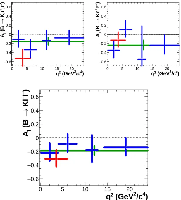
Figure 4. A

measurements in bins of q

, for decays B → Kµ

µ

(top-left), B → Ke

e

(top-right), and both modes combined (bottom). The legends are the same as in Fig. 3.

together, as we do not distinguish between B

and B ¯

. The total branching fraction

B( B

→ K

µ

e

) corresponds, via isospin invariance, to B( B

→ K

µ

e

)+B( B

→ K

µ

e

).

The significance of the signal yield for B

→ K

µ

e

channel is 2.8σ. To estimate the

signal significance for this mode, we have generated a large sample of pseudoexperiments

with N

= 0 and estimated the number of cases which have N

> N

(observed). The

confidence level obtained is then translated to significance. We calculate the upper limit for

these modes at 90% CL using a frequentist method. In this method, for different numbers

0 5 10 15 20 25

)

2

/c

2

(GeV q

0 0.1 0.2 0.3 0.4 0.5

) /c /GeV (10 dB/dq 0.6

0 5 10 15 20 25

4

)

2

/c

2

(GeV q

0 0.1 0.2 0.3 0.4 0.5

) /c /GeV (10 dB/dq 0.6

0 5 10 15 20 25

4

)

2

/c

2

(GeV q

0 0.1 0.2 0.3 0.4 0.5

) /c /GeV (10 dB/dq 0.6

0 5 10 15 20 25

4

)

2

/c

2

(GeV q

0 0.1 0.2 0.3 0.4 0.5

) /c /GeV (10 dB/dq 0.6

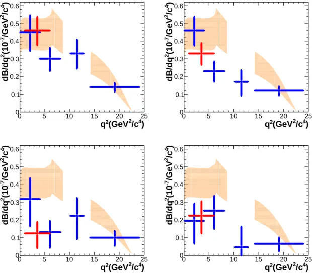
Figure 5. dB/dq

measurements in bins of q

, for decays B

→ K

µ

µ

(top-left), B

→ K

e

e

(top-right), B

→ K

µ

µ

(bottom-left), and B

→ K

e

e

(bottom-right). The legends are the same as in Fig. 3. The yellow shaded regions show the theoretical predictions from the light-cone sum rule and lattice QCD calculations [38, 39].

Table 2. Branching fraction for B → Kℓ

ℓ

and B → J/ψK decays.

Mode B

B

→ K

ℓ

ℓ

(5.99

± 0.14) × 10

B

→ K

ℓ

ℓ

(3.51

± 0.10) × 10

B

→ J/ψK

(1.032 ± 0.007 ± 0.024) × 10

B

→ J/ψK

(0.902 ± 0.010 ± 0.026) × 10

of signal events N

(gen), we generate 1000 Monte Carlo experiments with signal and back- ground PDFs, with each set of events being statistically equivalent to our data sample of

– 12 –

5.2 5.22 5.24 5.26 5.28 5.3

2) (GeV/c Mbc

1 10 102

103

104

)2Entries / (2 MeV/c

−0.1−0.05 0 0.05 0.1 0.15 0.2 0.25 E (GeV)

∆ 1

10 102

103

Entries / (5 MeV)

−8 −6 −4 −2 0 2 4 6 8 O’

1 10 102

103

Entries / (0.32)

2) (GeV/c Mbc

5.2 5.22 5.24 5.26 5.28 5.3 )2Entries / (2 MeV/c

1 10 102

103

104

E (GeV)

∆

−0.1−0.05 0 0.05 0.1 0.15 0.2 0.25

Entries / (5 MeV)

1 10 102

103

O’

−8 −6 −4 −2 0 2 4 6 8

Entries / (0.32)

1 10 102

103

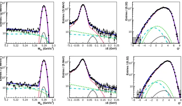
Figure 6. M

(left), ∆E (middle), and O

(right) projections of three-dimensional unbinned extended maximum-likelihood fits to the data events that pass the selection criteria for B

→ J/ψ(→ µ

µ

)K

(top), and B

→ J/ψ(→ e

e

)K

(bottom). The legends are the same as in Fig. 1 and black dashed curve is [π

J/ψ] background.

5.2 5.22 5.24 5.26 5.28 5.3

2) (GeV/c Mbc

0 20 40 60 )2Entries / (5.55556 MeV/c

5.2 5.22 5.24 5.26 5.28 5.3

2) (GeV/c Mbc

0 10 20 30 40 )2Entries / (5.55556 MeV/c

5.2 5.22 5.24 5.26 5.28 5.3

2) (GeV/c Mbc

0 10 20 30 )2Entries / (5.55556 MeV/c

Figure 7. Signal-enhanced M

projection of three-dimensional unbinned extended maximum- likelihood fits to the data events that pass the selection criteria for decays B

→ K

µ

e

(left), B

→ K

µ

e

(middle), and B

→ K

µ

e

(right). The legends are same as in Fig. 1.

711 fb

. We fit all these simulated data sets, and, for each value of N

(gen), we calculate the fraction of MC experiments that have N

≤ N

(data). The 90% CL upper limit is taken to be the value of N

(gen) (called here N

) for which 10% of the experiments have N

≤ N

(data). The upper limit on the branching fraction is then derived using the formula:

B

= N

N

× 2 × f

× ε ,

where N

is the number of B B ¯ pairs = (772 ± 11) × 10

, f

is the branching fraction B[Υ(4S) → B

B

] (B[Υ(4S) → B

B ¯

]) for charged (neutral) B decays, and ε is the signal reconstruction efficiency calculated from signal MC samples. The systematic uncertainty in B

is included by smearing the N

obtained from the MC fits with the fractional systematic uncertainty (discussed in Section 5). The results are listed in Table 3.

Table 3. Branching fraction UL calculation at 90% CL for LFV B → Kµe decays.

Mode ε (%) N

N

B

(10

) B

→ K

µ

e

29.4 11.6

19.9 8.5 B

→ K

µ

e

31.2 1.7

7.5 3.0 B

→ K

µ

e

20.9 −3.3

3.0 3.8

5 Systematic uncertainties

Systematic uncertainties arising due to lepton identification is 0.3% (0.4%) for each muon (electron) selection. This uncertainty is calculated using an inclusive J/ψ → ℓ

ℓ

, ℓ = e or µ sample. Uncertainty due to hadron identification is 0.8% for K

using D

→ D

(K

π

)π

sample and 1.6% for K

[35]. The systematic uncertainty due to charged track reconstruction is 0.35% per track estimated by using the partially reconstructed D

→ D ¯

π

, D ¯

→ π

π

K

, and K

→ π

π

events. The uncertainty in effi- ciency due to limited MC statistics is about 0.2%, and the uncertainty in the number of B B ¯ events is 1.4%. The systematic uncertainty in the branching fraction B[Υ(4S) → B

B

] (B[Υ(4S) → B

B ¯

]) is 1.2% [9]. We compare the efficiency of the O > O

crite- rion between data and MC samples with the control channel B → J/ψK, J/ψ → ℓ

ℓ

; the differences between data and MC simulation (0.9-1.2%) are corrected and the correspond- ing uncertainty (0.2-0.3%) is assigned as a systematic uncertainty. The uncertainty due to PDF shapes is evaluated by varying the fixed shape parameters by ±1σ and repeating the fit; the change in the central value of N

is taken as the systematic uncertainty, which ranges from 0.1 to 0.6%. The uncertainty due to the fixed yield of continuum events is estimated by varying the yield by ±1σ in the fit; the resulting variation in N

is less than 1%. The charmless B → Kπ

π

background fixed in the fit for the modes with muon final states is varied within ±1σ in the fit, and the change in N

is assigned as system- atic, which is 0.1-0.2%. The decay model systematic for B → Kℓ

ℓ

modes is evaluated by comparing reconstruction efficiencies calculated from MC samples generated with dif- ferent models [36, 37] and is 0.3 to 2.0% depending on the q

bin. For the B → J/ψK branching fraction, we have considered all the sources except for the contribution due to fixed continuum or charmless B → Kπ

π

events and the decay model. The systematic uncertainties such as hadron identification, track reconstruction, number of B B ¯ events, and the ratio B[Υ(4S) → B

B

] (B[Υ(4S) → B

B ¯

]) cancel out in the double ratio of R

(J/ψ), while for A

(J/ψK) the sources that divide out are lepton identification and number of B B ¯ events as listed in Table 4. In the case of R

, systematic uncertainties

– 14 –