1
Temporal dynamics of surface ocean carbonate chemistry in response
1
to natural and simulated upwelling events during the 2017 coastal El
2
Niño near Callao, Peru
3
Shao-Min Chen1, 2, Ulf Riebesell1, Kai G. Schulz3, Elisabeth von der Esch1, Eric P. Achterberg1, and 4
Lennart T. Bach4 5
1GEOMAR Helmholtz Centre for Ocean Research Kiel, Kiel, Germany 6
2Department of Earth and Environmental Sciences, Dalhousie University, Halifax, Canada 7
3Centre for Coastal Biogeochemistry, School of Environment, Science and Engineering, Southern Cross University, Lismore, 8
Australia 9
4Institute for Marine and Antarctic Studies, University of Tasmania, Tasmania, Australia 10
11
Correspondence to: Shao-Min Chen (shaomin.chen@dal.ca) 12
Abstract. Oxygen minimum zones (OMZs) are characterized by enhanced carbon dioxide (CO2) levels and low pH and are 13
being further acidified by uptake of anthropogenic atmospheric CO2. With ongoing intensification and expansion of OMZs 14
due to global warming, carbonate chemistry conditions may become more variable and extreme, particularly in the Eastern 15
Boundary Upwelling Systems. In austral summer (Feb-Apr) 2017, a large-scale mesocosm experiment was conducted in the 16
coastal upwelling area off Callao (Peru) to investigate the impacts of on-going ocean deoxygenation on biogeochemical 17
processes, coinciding with a rare coastal El Niño event. Here we report on the temporal dynamics of carbonate chemistry in 18
the mesocosms and surrounding Pacific waters over a continuous period of 50 days with high temporal resolution observations 19
(every 2nd day). The mesocosm experiment simulated an upwelling event in the mesocosms by addition of nitrogen (N)- 20
deficient and CO2-enriched OMZ water. Surface water in the mesocosms was acidified by the OMZ water addition, with pHT
21
lowered by 0.1-0.2 and pCO2 elevated to above 900 μatm. Thereafter, surface pCO2 quickly dropped to near or below the 22
atmospheric level (405.22 μatm in 2017, NOAA/GML) mainly due to enhanced phytoplankton production with rapid CO2
23
consumption. Further observations revealed that the dominance of dinoflagellate Akashiwo sanguinea and contamination of 24
bird excrements played important roles in the dynamics of carbonate chemistry in the mesocosms. Compared to the simulated 25
upwelling, natural upwelling events in the surrounding Pacific waters occurred more frequently with sea-to-air CO2 fluxes of 26
4.2-14.0 mmol C m-2 d-1.The positive CO2 fluxes indicated our site was a local CO2 source during our study, which may have 27
been impacted by the coastal El Niño. However, our observations of DIC drawdown in the mesocosms suggests that CO2
28
fluxes to the atmosphere can be largely dampened by biological processes. Overall, our study characterized carbonate 29
chemistry in near-shore Pacific waters that are rarely sampled in such temporal resolution and hence provided unique insights 30
into the CO2 dynamics during a rare coastal El Niño event.
31
1 Introduction 32
One of the most extensive oxygen minimum zones (OMZs) in the global ocean can be found off central/northern Peru (4 - 16°
33
S, Chavez and Messié, 2009). High biological productivity is stimulated by permanent upwelling of cold, nutrient-rich water 34
to the surface supporting a remarkable fish production off Peru (Chavez et al., 2008; Montecino and Lange, 2009; Albert et 35
al., 2010). The high primary production also leads to enhanced remineralization of sinking organic matter in subsurface waters 36
which depletes dissolved oxygen (O2) and creates an intense and shallow OMZ (Chavez et al., 2008). The depletion of O2 in 37
OMZs plays an important role in the global nitrogen (N) cycle, accounting for 20 - 40% N loss in the ocean (Lam et al., 2009;
38
Paulmier and Ruiz-Pino, 2009). Denitrification and anammox processes that occur in O2 depleted waters remove N from the 39
ocean and produce an N deficit and hence phosphorus (P) excess with respect to the Redfield ratio (C:N:P = 106:16:1) in the 40
water column (Redfield, 1963; Deutsch et al., 2001; Deutsch et al., 2007; Hamersley et al., 2007; Galán et al., 2009; Lam et 41
al., 2009). Upwelling of this N-deficient water has been found to control the surface-water nutrient stoichiometry and thus 42
influence phytoplankton growth and community compositions (Franz et al., 2012; Hauss et al., 2012).
43
Apart from being N-deficient, the OMZ waters are also characterized by enhanced carbon dioxide (CO2) concentrations and 44
low pH from respiratory processes and are further acidified by uptake of anthropogenic atmospheric CO2 (Feely et al., 2008;
45
Friederich et al., 2008; Paulmier et al., 2008; Paulmier et al., 2011). Accordingly, surface water carbonate chemistry is 46
influenced by upwelling of CO2-enriched OMZ water (Van Geen et al., 2000; Capone and Hutchins, 2013). The upwelled 47
CO2-enriched OMZ water can give rise to surface CO2 levels >1,000 µatm, pH values as low as 7.6, and under-saturation for 48
the calcium carbonate mineral aragonite (Feely et al., 2008; Hauri et al., 2009). As a result, there is a significant flux of CO2
49
from the ocean to the atmosphere off Peru, which is further facilitated by surface ocean warming, making the Peruvian 50
upwelling region a year-round CO2 source to the atmosphere (Friederich et al., 2008). In contrast, rapid utilization of upwelled 51
3
CO2 and nutrients by phytoplankton can occasionally deplete surface CO2 below atmospheric equilibrium and dampen the CO2
52
outgassing (Van Geen et al., 2000; Friederich et al., 2008; Loucaides et al., 2012). The enhanced primary production in turn 53
contributes to increasing export of organic matter, enhanced bacterial respiration, O2 consumption and CO2 production at 54
depth. Such a positive feedback may determine the intensity of the underlying OMZ and promote carbon (C) preservation in 55
marine sediments (Dale et al., 2015).
56
In response to reduced O2 solubility and enhanced stratification induced by global warming, OMZs have been intensifying and 57
expanding over the past decades (Stramma et al., 2008; Fuenzalida et al., 2009; Stramma et al., 2010). Based on regional 58
observations and model projections, a decline in dissolved O2 concentrations has been reported for most regions of the global 59
ocean (Matear et al., 2000; Matear and Hirst, 2003; Whitney et al., 2007; Stramma et al., 2008; Keeling et al., 2009; Bopp et 60
al., 2013; Schmidtko et al., 2017; Oschlies et al., 2018). The vertical expansion of OMZs represents shoaling of CO2-enriched 61
seawater, which has become further enriched by oceanic uptake of anthropogenic CO2 (Doney et al., 2012; Gilly et al., 2013;
62
Schulz et al., 2019). Since biogeochemical processes in OMZs are directly linked to the C cycle and control surface nutrient 63
stoichiometry, with on-going ocean warming and acidification, the deoxygenation may have cascading effects on plankton 64
productivity and composition, C uptake, and food web functioning (Keeling et al., 2009; Gruber, 2011; Doney et al., 2012;
65
Gilly et al., 2013; Levin and Breitburg, 2015). Therefore, it is important to monitor the changes in CO2 when investigating the 66
effects of deoxygenation on marine ecosystems.
67
To investigate the potential impacts of upwelling on pelagic biogeochemistry and natural plankton communities in the Peruvian 68
OMZ, a large-scale in situ mesocosm study was carried out in the coastal upwelling area off Peru. An upwelling event was 69
simulated in the mesocosms by addition of OMZ waters collected from two different locations where the OMZ was considered 70
to contain different nutrient concentrations and N:P ratios. The ecological and biogeochemical responses in the mesocosms 71
were monitored and compared with those influenced by natural upwelling events in the ambient coastal water surrounding the 72
mesocosms. As part of this collaborative research project, questions specific to the present paper were: (1) How does surface 73
water carbonate chemistry respond to an upwelling event?; and (2) How does upwelled OMZ water with different chemical 74
signatures modulate surface water carbonate chemistry? The current study will mainly focus on the temporal changes in surface 75
water carbonate chemistry within the individual mesocosms, including observations made in the ambient Pacific water and a 76
local estimate of air-sea CO2 exchange, together with the influence by a rare coastal El Nino event (Garreaud, 2018). This 77
provides first insights into how inorganic C cycling links to chemical signatures of OMZ waters in a natural plankton 78
community and its implications for ongoing environmental changes.
79
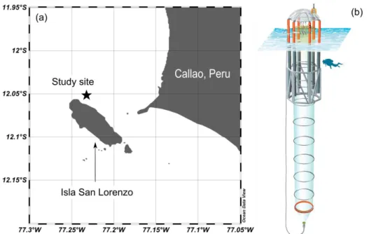
2 Material and methods 80
2.1 Study site 81
The experiment was conducted in the framework of the Collaborative Research Center 754 "Climate-Biogeochemistry 82
Interactions in the Tropical Ocean" (www.sfb754.de/en) and in collaboration with the Instituto del Mar del Peru (IMARPE) 83
in Callao, Peru (Fig. 1a). The coastal area off Callao lies within the Humboldt Current System and is influenced by wind- 84
induced coastal upwelling (Bakun and Weeks, 2008).
85
2.2 Mesocosm setup 86
Eight “Kiel Off-Shore Mesocosms for Future Ocean Simulations” (KOSMOS) units (M1-M8), extending 19 m below the sea 87
surface, were deployed by the research vessel Buque Armada Peruana (BAP) Morales and moored at 12.06° S, 77.23° W in 88
the coastal upwelling area off Callao, Peru (Fig. 1a) on February 23rd, 2017 (late austral summer). The technical design of 89
these sea-going mesocosms is described by Riebesell et al. (2013). For a more detailed description of the mesocosm 90
deployment and maintenance in this study, please refer to Bach et al. (2020a).
91
The mesocosm bags were filled with surrounding seawater through the upper and lower openings. Both openings were covered 92
by screens with a mesh size of 3 mm to avoid enclosing larger organisms such as fish. The mesocosm bags were left open 93
below the water surface for two days, allowing free exchange with surrounding coastal water. On February 25th, mesocosm 94
bags were closed with the screens removed, tops pulled above the sea surface and bottoms sealed with 2-m long conical 95
sediment traps (Fig. 1b). The experiment started with the closure of the mesocosms (day 0) and lasted for 50 days. Each 96
mesocosm bag enclosed a seawater volume of ~54 m3. After the bags were closed, daily or every-2nd-day sampling was 97
performed to monitor the initial conditions of the enclosed water before simulating an upwelling event on day 11 and 12 (see 98
Sect. 2.4 for details).
99
100
Figure 1 The study site of the mesocosm experiment (a) created and modified using Ocean Data View (Schlitzer, Reiner, Ocean 101
Data View, odv.awi.de, 2021) and a schematic illustration of a KOSMOS mesocosm unit (b). We acknowledge reprint permission 102
from the AGU as parts of this drawing was used for a publication by Bach et al. (2016). The star symbol marks the approximate 103
location of mesocosm deployment.
104
2.3 Simulated upwelling and salt addition 105
To simulate an upwelling event in the mesocosms, OMZ-influenced waters were collected from the nearby coastal area and 106
added to the mesocosms. Two OMZ water masses were collected at Station 1 (12° 01.70’ S, 77° 13.41’ W) at a depth of ~30 107
m and at Station 3 (12° 02.41’ S, 77° 22.50’ W) at a depth of ~70 m respectively using a deep-water collection system as 108
described by Taucher et al. (2017). These two water masses were sampled for chemical and biological variables as the 109
mesocosms (see Sect. 2.4). The OMZ water collected from Station 3 had a dissolved inorganic nitrogen (DIN) concentration 110
of 4.3 μmol L-1 (denoted as “Low DIN” in this paper) and was added to M2, M3, M6 and M7. The OMZ water from Station 1 111
had a DIN of 0.3 μmol L-1 (denoted as “Very low DIN” in this paper) and was added to M1, M4, M5 and M8. Before OMZ 112
water addition, approximately 9 m3 of seawater were removed from 11-12 m of each mesocosm on March 5th (day 8). During 113
the night of March 8th (day 11), ~10 m3 of OMZ water were added to 14-17 m of each mesocosm. On March 9th (day 12), ~10 114
m3 of seawater were removed from 8-9 m followed by an addition of ~12 m3 OMZ water to 0-9 m of each mesocosm.
115
5
To maintain a low-O2 bottom layer in the mesocosms and avoid convective mixing induced by heat exchange with the 116
surrounding Pacific, 69 L of a concentrated sodium chloride (NaCl) brine solution were added to the bottom of each mesocosm 117
(10-17 m) on day 13, which increased the bottom salinity by ~0.7 units. Since then, turbulent mixing induced by sampling 118
activities continuously interrupted the artificial halocline. Hence, on day 33, 46 L of the NaCl brine solution were added again 119
to the bottom of each mesocosm (12.5-17 m), which increased the bottom salinity by ~0.5 units. At the end of the experiment 120
after the last sampling (day 50), 52 kg of NaCl brine was added again to each mesocosm to calculate the enclosed seawater 121
volume from a measured salinity change by ~0.2 units (see Czerny et al., 2013 and Schulz et al., 2013 for details). The average 122
final volume for each mesocosm bag was calculated at ~54 m3. With known sampling volumes and deep-water addition 123
volumes during the experiment, the enclosed volumes of each mesocosm on each sampling day could be calculated. The NaCl 124
solution for the halocline establishments had been prepared in Germany by dissolving 300 kg of food industry grade NaCl 125
(free of anti-caking agents) in 1000 L deionized water (Milli-Q, Millipore) and purified with ion exchange resin (LewawitTM 126
MonoPlus TP260®, Lanxess, Germany) to minimize potential contaminations with trace metals (Czerny et al., 2013). The 127
NaCl solution for the volume determination was produced on site using locally purchased table salt. For a more detailed 128
description of OMZ water and salt additions, please refer to Bach et al. (2020a).
129
2.4 Sampling procedures and CTD operations 130
Sampling was carried out in the morning (7 a.m.-11 a.m. local time) daily or every 2nd day throughout the entire experimental 131
period. Depth-integrated samples were taken from the surface (0-10 m for day 3-28) and bottom layer (10-17 m for day 3-28) 132
of the mesocosms and the surrounding coastal water (named “Pacific”) using a 5-L integrating water sampler (IWS, HYDRO- 133
BIOS, Kiel). Due to the deepening of the oxycline as observed from the CTD profiles, the sampling depth for the surface was 134
adjusted to 0-12.5 m while that for the bottom was changed to 12.5-17 m from day 29 until the end of the experiment (day 50).
135
For gas-sensitive variables such as pH and dissolved inorganic carbon (DIC), 1.5 L of seawater from each integrated depth in 136
each mesocosm were taken directly from the fully-filled 5-L integrating water sampler. Clean polypropylene sampling bottles 137
(rinsed with deionized water in the laboratory; Milli-Q, Millipore) were pre-rinsed with sample water immediately prior to 138
sampling. Bottles were filled from bottom to top using pre-rinsed Tygon tubing with overflow of at least one sampling bottle 139
volume (1.5 L) to minimize the impact of CO2 air-water gas exchange. Nutrient samples were collected into 250 ml 140
polypropylene bottles using pre-rinsed Tygon tubing (see Bach et al., 2020a for details). Sample containers were stored in cool 141
boxes for ~3 hours, protected from sunlight and heat before being transported to the shore. Once in the lab, sample water was 142
sterile-filtered by gentle pressure using syringe filters (0.2 μm pore size), Tygon tubing and a peristaltic pump to remove 143
particles that may cause changes to seawater carbonate chemistry (Bockmon and Dickson, 2014). For DIC measurements, the 144
water was filtered from the bottom of the 1.5-L sample bottle into 100-ml glass-stoppered bottles (DURAN) with an overflow 145
of at least 100 ml to minimize contact with air. Once the glass bottle was filled with sufficient overflow, it was immediately 146
sealed without headspace using a round glass stopper. This procedure was repeated to collect a second bottle (100 ml) of 147
filtered water for pH measurements. The leftover seawater was directly filtered into a 500 ml polypropylene bottle for total 148
alkalinity (TA) measurements (non-gas-sensitive). Filtered DIC and pH samples were stored at 4 ℃ in the dark and TA samples 149
were at room temperature in the dark until further analysis. Samples were analysed for DIC and pH on the same day of 150
sampling, while TA was determined overnight (see Sect. 2.5 for analytical procedures).
151
CTD casts were performed with a multiparameter logging probe (CTD60M, Sea and Sun Technology) in the mesocosms and 152
Pacific on every sampling day. From the CTD casts, profiles of salinity, temperature, pH, dissolved O2, chlorophyll a (chl a) 153
and photosynthetically active radiation were obtained (see Schulz and Riebesell, 2013 and Bach et al., 2020a for details).
154
2.5 Carbonate chemistry and nutrient measurements 155
Total alkalinity was determined at room temperature (22-32℃) by a two-stage open-cell potentiometric titration using a 156
Metrohm 862 Compact Titrosampler, Aquatrode Plus (Pt1000) and a 907 Titrando unit in the IMARPE laboratory following 157
Dickson et al. (2003). The acid titrant was prepared by preparing a 0.05 mol kg-1 hydrochloric acid (HCl) solution with an 158
ionic strength of ca. 0.7 mol kg-1 (adjusted by NaCl). Approximately 50-grams of sample water from each sample was weighed 159
into the titration cell with the exact weight recorded (precision: 0.0001 g). After the two-stage titration, the titration data 160
between a pH of ~3.5 and 3 was fitted to a modified non-linear Gran approach described in Dickson et al. (2007) using 161
MATLAB (The MathWorks). The results were calibrated against certified reference materials (CRMs) batch 142 (Dickson, 162
2010) measured on each measurement day. In this paper, measured TA values refer to the measured values that have been 163
calibrated against the CRM.
164
Seawater pHT (total scale) was determined spectrophotometrically by measuring the absorbance ratios after adding the 165
indicator dye m-cresol purple (mCP) as described in Carter, et al. (2013). Before measurements, samples were acclimated to 166
25.0°C in a thermostatted bath. The absorbance of samples with mCP was determined on a Varian-Cary 100 double-beam 167
spectrophotometer (Varian), scanning between 780 and 380 nm at 1-nm resolution. During the spectrophotometric 168
measurement, the temperature of the sample was maintained at 25.0°C by a water-bath connected to the thermostatted 10-cm 169
cuvette. The pHT values were calculated from the baseline-corrected absorbance ratios and corrected for in situ salinity 170
(obtained from CTD casts) and pH change caused by dye addition (using the absorbance at the isosbestic point, i.e. 479 nm) 171
as described in Dickson et al. (2007). To minimize potential CO2 air-water gas exchange, a syringe pump (Tecan Cavro XLP) 172
was used for sample/dye mixing and cuvette injection (see Schulz et al. 2017 for details). For the dye correction, a batch of 173
sterile filtered seawater of known salinity was prepared. The pHT was determined once for an addition of 7 ul of dye and once 174
of 25 ul at five pH levels (raised to 7.95 with NaOH and lowered to 7.74, 7.58, 7.49 and 7.36 with HCl stepwise). The pH 175
change resulting from the dye correction addition was calculated from the change in measured absorbance ratio for each pair 176
of dye additions (see Clayton and Byrne, 1993 and Dickson et al., 2007 for details). The dye-corrected pHT values measured 177
at 25.0°C and atmospheric pressure were then re-calculated for in situ temperature and pressure as determined by CTD casts 178
(averaged over 0-10/12.5 m for surface and 10/12.5-17 m for bottom). For carbonate chemistry speciation calculations (see 179
Sect. 2.6), the dye-corrected pHT values were used as one of the input parameters.
180
Dissolved inorganic carbon was measured by infrared absorption using a LI-COR LI-7000 on an AIRICA system 181
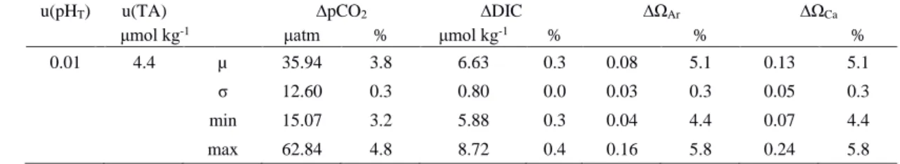
(MARIANDA, Kiel, see Taucher et al., 2017 and Gafar and Schulz, 2018 for details). The results were calibrated against 182
CRMs batch 142 (Dickson, 2010). Unfortunately, due to a malfunctioning of the AIRICA system, we obtained measured DIC 183
data only up to March 7th (day 10). Therefore, measured TA and pHT were used for calculations of carbonate system 184
parameters at in situ temperature and salinity but we used DIC measurements from day 3-10 for consistency checks of 185
calculated carbonate chemistry parameters. In this paper, measured DIC values refer to the measured values that have been 186
calibrated against the CRM.
187
Inorganic nutrients were analyzed colorimetrically (NO3-, NO2-, PO43- and Si(OH)4) and fluorimetrically (NH4+) using a 188
continuous flow analyzer (QuAAtro AutoAnalyzer with integrated photometers, SEAL Analytical) connected to a fluorescence 189
detector (FP-2020, JASCO). All colorimetric methods were conducted according to Murphy and Riley (1962), Mullin and 190
Riley (1955a, b) and Morris and Riley (1963) and corrected following the refractive index method developed by Coverly et al.
191
(2012). For details of the quality control procedures, see Bach et al. (2020a).
192
7
2.6 Carbonate chemistry speciation calculations and propagated uncertainties 193
Calculations of carbonate chemistry parameters (in situ pHT, DIC, pCO2,and calcium carbonate saturation state for calcite and 194
aragonite) were performed with the Excel version of CO2SYS (Version 2.1, Pierrot et al., 2006) using K1 and K2 dissociation 195
constants from Mehrbach et al., (1973) which were refitted by Lueker et al. (2000). The dissociation constant for KHSO4 from 196
Dickson (1990) and for total boron from Uppström (1974) were applied in the calculations (see Orr et al., 2015 for details).
197
The observed pHT and TA as well as inorganic nutrient concentration (phosphate and silicic acid) were used as input CO2
198
system parameters. In situ salinity and temperature were obtained by CTD casts and averaged over surface (0-10 m or 0-12.5 199
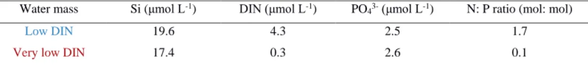
m) and bottom (10-17 m or 12.5-17 m) waters for each sampling day. In situ pressure was approximated for surface (5 dbar) 200
and bottom (13.5 or 14.75 dbar) waters. For details of calculation procedures and choices of constants, see Lewis et al. (1998) 201
and Orr et al. (2015).
202
To evaluate the performance of pHT and TA measurements, quality control procedures were performed. First, standard 203
deviations of pHT measurements were graphed over time. Measured TA values of a control sample (CRM batch 142, Dickson, 204
2010) were plotted over time, compared to the warning and control limits calculated from their mean and standard deviation 205
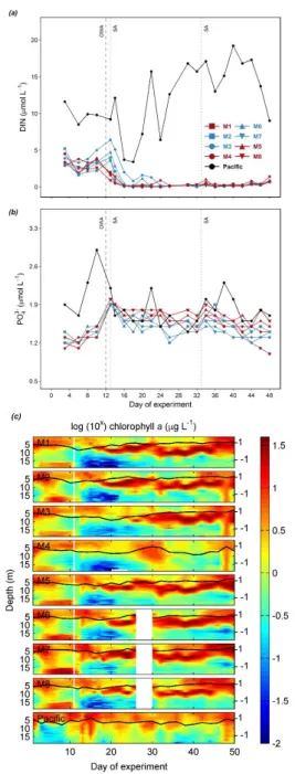
(for details please see Dickson et al., 2007) as well as the certified value of the CRM. To compute a range control chart for the 206
evaluation of measurement repeatability, the absolute difference between duplicate measurements of CRMs on each sampling 207
day was calculated and plotted over time, compared to the warning and control limits calculated from their mean and standard 208
deviation (for details see Dickson et al., 2007).
209
We used the R package seacarb with a Gaussian approach and an input variable pair (pHT, TA) to calculate uncertainties for 210
calculated CO2 system parameters (Orr et al. 2018; Gattuso et al. 2020). The contribution of input uncertainties in nutrient 211
concentrations and in situ salinity and temperature to the uncertainties in the CO2SYS-based calculations are often small (<
212
0.1%; Orr et al. 2018) so they were not considered in our propagation. The input uncertainties of pHT and TA were estimated 213
based on our measurements (Table 1). Standard uncertainties include random and systematic errors. For TA, systematic errors 214
were removed by calibrating the measured results using CRMs (see Sect. 2.5). Hence, the random error of TA, estimated by 215
the averaged standard deviation of all the CRM measurements (4.4 μmol kg-1; n = 62), was used as the standard uncertainty.
216
For pHT, an uncertainty of 0.01 was used as the standard uncertainty. Due to the unavailability of CRMs that correct for 217
systematic error in pH measurements, the standard deviations of repeated measurements (0.0012; n = 377) only accounted for 218
the random components of standard uncertainties (Orr et al. 2018). Therefore, we used 0.01 in our uncertainty propagation as 219
an approximation of the total standard uncertainty for pHT, which has been used in previous assessments (Orr et al. 2018).
220
Table 1: Standard uncertainties of pHT and TA estimated based on our measurements are denoted by u(pHT) and u(TA). Based 221
on u(pHT) and u(TA), propagated uncertainties were estimated for each data point in R and averaged for each reported variable 222
(µ), with Standard deviation (σ), minimum (min) and maximum (max) values presented. The relative percentage (%) of 223
propagated standard uncertainties were calculated by dividing the propagated uncertainty by the corresponding data point and 224
averaged for each reported variable (µ), with σ, min and max values presented.
225
u(pHT) u(TA) ∆pCO2 ∆DIC ∆ΩAr ∆ΩCa
μmol kg-1 μatm % μmol kg-1 % % %
0.01 4.4 µ 35.94 3.8 6.63 0.3 0.08 5.1 0.13 5.1
σ 12.60 0.3 0.80 0.0 0.03 0.3 0.05 0.3
min 15.07 3.2 5.88 0.3 0.04 4.4 0.07 4.4
max 62.84 4.8 8.72 0.4 0.16 5.8 0.24 5.8
The air-sea flux of CO2 (FCO2, mmol C m-2 d-1) in the Pacific was determined based on 226
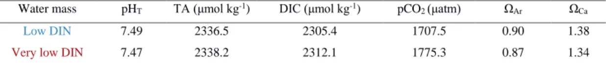
𝐹𝐶𝑂2 = 𝑘 𝐾0 ∆𝑝𝐶𝑂2 (1)
227
where k is the gas transfer velocity parameterized as a function of wind speed, K0 is the solubility of CO2 in seawater dependent 228
on in situ salinity and temperature (Weiss, 1974), and ∆pCO2 is the difference between pCO2 in the surface water and in the 229
atmosphere (Wanninkhof 2014). Wind data were averaged over 2 sampling days for the sampling location from a satellite- 230
derived gridded dataset (GLDAS Model, near surface wind speed, 0.25 x0.25 degrees, 3 hour temporal resolution, 12.375° to 231
11.875°S, 77.375° to 76.875°W), obtained from NASA Giovanni (Rodell et al., 2004; Beaudoing and Rodell, 2020). In situ 232
salinity and temperature were obtained from the CTD casts (see Sect. 2.4). Calculated pCO2 based on (pHT, TA) and an 233
estimated atmospheric pCO2 of 405.22 μatm (referenced to year 2017, NOAA/GML) were used in the air-sea flux estimation.
234
3 Results 235
3.1 Responses of surface layer nutrient concentrations 236
The OMZ-influenced water masses were collected from two locations and added to the mesocosms to simulate an upwelling 237
event (see Sect. 2.3). The two water masses were named “Low DIN” and “Very low DIN” respectively based on their DIN 238
concentrations (Table 2). Both water masses shared similar silicic acid (Si) and phosphate (PO43-) concentrations but differed 239
in DIN concentration. The “Low DIN” water had a DIN concentration of 4.3 μmol L-1, 14 times as high as that of the “Very 240
low DIN” water (0.3 μmol L-1; Table 2).
241
9
Table 2: Inorganic nutrient concentrations of the two collected deep-water masses. Please note that DIN is the sum of nitrate, nitrite 242
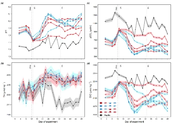
and ammonium. P is phosphate. Si is silicic acid. Color codes denote the two water masses and are applied to the mesocosms treated 243
with respective water masses in the following figures and tables.
244
Water mass Si (μmol L-1) DIN (μmol L-1) PO43- (μmol L-1) N: P ratio (mol: mol)
Low DIN 19.6 4.3 2.5 1.7
Very low DIN 17.4 0.3 2.6 0.1
On day 10 before OMZ water addition, the average surface DIN concentration of the two treatment groups were similar (3.4 245
μmol L-1), but lower than that in the Pacific (9.8 μmol L-1; Table 3). Surface layer DIN concentration in the mesocosms ranged 246
between 2.0 and 6.0 μmol L-1 before OMZ water addition (Fig. 2a). The addition of OMZ water elevated surface DIN in the 247
“Low DIN” mesocosms to 3.6-6.4 μmol L-1 but lowered that in the “Very low DIN” to 0.9-2.0 μmol L-1. The average surface 248
DIN concentration in the “Very low DIN” decreased to 1.6 μmol L-1 while the “Low DIN” slightly increased to 4.7 μmol L-1 249
(Table 3), followed by a sharp depletion on day 16 except for M3. M3 received the highest input of DIN (6.4 μmol L-1) and 250
was not depleted until day 24. Despite several small peaks in M3, M4, M5 and M6 (≤ 1.6 μmol L-1), surface DIN concentration 251
in the mesocosms were at around limits of detection (LODs: NH4+ = 0.063 µmol L-1, NO2- = 0.054 µmol L-1, NO3- = 0.123 252
µmol L-1) most of the time after depletion. A slight rise could be observed from day 44 towards the last sampling day (day 48).
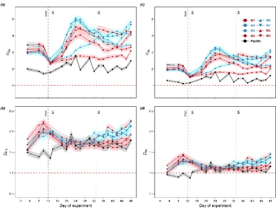
253
In the Pacific, surface layer DIN concentration was mostly greater than 5 μmol L-1 (except on day 16 and 18) and became 254
considerably higher during the second half of the experiment (> 10 μmol L-1 for day 26-44; Fig. 2a).
255
Table 3: DIN concentration (μmol L-1) in the surface layer of each mesocosm (M1-M8) and the average DIN concentration (μmol L- 256
1) for each treatment (“Low DIN” and “Very Low DIN”, n = 4) before (t10) and after deep water addition (t13). The DIN 257
concentration in the surface Pacific water is also shown. Color codes and symbols denote the respective mesocosm in the following 258
figures.
259
M1 M2 M3 M4 M5 M6 M7 M8 Low DIN Very Low DIN Pacific
t10 3.7 2.2 5.0 3.3 3.9 3.4 3.2 2.6 3.4 ± 1.2 3.4 ± 0.5 9.8
t13 1.8 3.6 6.4 2.0 1.6 4.7 4.0 0.9 4.7 ± 1.3 1.6 ± 0.5 9.2
Surface layer PO43- concentrations in the mesocosms initially ranged between 1.1 and 1.5 μmol L-1 and were elevated by OMZ 260
water addition to around 1.9 μmol L-1 (Fig. 2b). Thereafter, PO43- exhibited a slow but steady decline until the end of the study 261
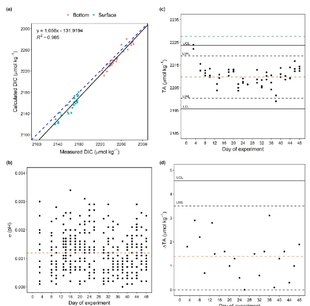
with a slightly higher decrease in “Low DIN” mesocosms (blue symbols; Fig. 2b). Throughout the study, PO43- in the 262
mesocosms was never lower than 1.1 μmol L-1. Surface layer PO43- in the Pacific was generally higher, fluctuating between 263
1.4 and 2.9 μmol L-1. In the mesocosms, enhanced chl a concentrations were observed at depths shallower than 5 m and below 264
15 m before OMZ water addition (Fig. 2c). Following OMZ water addition, a chl a maximum occurred at ~10 m and persisted 265
until day 40, except for M3 and M4 with a 1-week delayed increase in the former and a lack of bloom in the latter (Fig. 2c).
266
After day 40, chl a concentrations in all mesocosms (except for M4) increased to 12-38 μg L-1 with a bloom occurring in 0-10 267
m (Fig. 2c) Throughout the study, a chl a maximum was continuously observed above 10 m in the Pacific (Fig. 2c).
268
269
Figure 2 Temporal dynamics of depth-integrated surface DIN concentration (a), PO43- concentration(b) and vertical distribution of 270
chl a concentration determined by CTD casts (c). The black solid lines on top of the coloured contours represent the average values 271
over the entire water column, with the corresponding additional y-axes on the right. The vertical white lines represent the day when 272
OMZ water was added to the mesocosms. Color codes and symbols denote the respective mesocosm. Abbreviation: OWA, OMZ 273
water addition. SA, salt addition. Dataset is available at https://doi.pangaea.de/10.1594/PANGAEA.923395 (Bach et al., 2020b).
274
3.2 Temporal dynamics of carbonate chemistry 275
Before OMZ water addition, surface layer pHT in the mesocosms ranged between 7.80-7.94 with a slight decline by ~0.1 over 276
time (Fig. 3a). The initial surface layer TA ranged between 2,310 and 2,330 μmol kg-1 (Fig. 3b; day 3-12). Surface layer pCO2
277
and DIC ranged from 541 to 749 μatm and 2,119 to 2,180 μmol kg-1, respectively (Fig. 3c, d).
278
11
The two collected OMZ-water masses shared similar carbonate chemistry properties despite the differences in DIN 279
concentrations. In both water masses, pHT was ~7.48, DIC was ~2,305-2,310 μmol kg-1, TA was ~2,337 μmol kg-1, and pCO2
280
was between 1,700 and 1,780 μatm (Table 4).
281
Table 4: The in situ pHT, TA, DIC, pCO2, ΩAr and ΩCa of the two collected OMZ-water masses.
282
Water mass pHT TA (μmol kg-1) DIC (μmol kg-1) pCO2 (μatm) ΩAr ΩCa
Low DIN 7.49 2336.5 2305.4 1707.5 0.90 1.38
Very low DIN 7.47 2338.2 2312.1 1775.3 0.87 1.34
Surface DIC and pCO2 were elevated from ~2,150 μmol kg-1 and ~600 μatm to ~2,200 μmol kg-1 and ~900 μatm (except M7) 283
by OMZ water addition, respectively, without distinct differences between the two treatments (Mann-Whitney U-Test, p >
284
0.05; Fig. 3c). Following OMZ water addition, surface pCO2 in the mesocosms decreased quickly and reached minima at 340- 285
500 μatm (except M3 and M4) on day 24 and 26. These minima corresponded with DIC minima at 2,040-2,110 μmol kg-1 and 286
pHT maxima at 7.9-8.1 (except M3 and M4; Fig. 3c, d). After reaching the minima, surface layer pCO2 exhibited a steady 287
increase to 410- 680 μatm from day 24 to day 38 and later declined in M3, M5, and M7 while the rest remained relatively 288
stable until day 42 (Fig. 3c). Interestingly, and unlike the other mesocosms, after OMZ water addition, pCO2 in M3 steadily 289
declined from 928 to 342 μatm until the end of the experiment while that in M4 remained constantly higher than the other 290
mesocosms (> 700 μatm), with a slightly decreasing trend to 645 μatm towards the end of the study (Fig. 3c).
291
In the Pacific, much lower surface pHT and higher surface pCO2 and DIC were observed compared to the mesocosms, with an 292
average of 7.7 (7.6-7.8), 1,078 μatm (775 – 1358 µatm) and 2,221 μmol kg-1 (2173 – 2269 µmol kg-1; minimum to maximum 293
range in parenthesis; Fig. 3c, d), respectively. TA in the Pacific was initially similar to that in the mesocosms, fluctuating 294
between 2,310 and 2,330 μmol kg-1, and later decreased to ~2,310 μmol kg-1 for the rest of the study.
295
Surface waters in the mesocosms and the Pacific were always saturated with respect to calcite and aragonite throughout the 296
entire experimental period, with lower values observed in the Pacific (Fig. 4a, c). Bottom waters in the mesocosms and Pacific 297
were always saturated with respect to calcite during the experiment (Fig. 4b) while bottom waters in the Pacific were 298
undersaturated with respect to aragonite before day 13 (0.88-0.99) and had ΩAr values slightly above 1.0 for the rest of the 299
study period (Fig. 4d).
300
301
Figure 3 Temporal dynamics of measured depth-integrated surface pHT (a) and TA (b), and calculated pCO2 (c) and DIC (d). The 302
error ribbons present measurement and propagated standard uncertainties of the calculations, respectively. Color codes and 303
symbols denote the respective mesocosm. Abbreviation: OWA, OMZ water addition. SA, salt addition.
304
13 305
Figure 4 Temporal dynamics of depth-integrated surface calcite saturation state (a), bottom calcite saturation state (b), surface 306
aragonite saturation state (c), and bottom aragonite saturation state (d) in the mesocosms and the surrounding Pacific. The error 307
ribbons present the propagated standard uncertainties of the calculations. When Ω > 1 (above red dashed line), seawater is 308
supersaturated for calcium carbonate. When Ω < 1 (below red dashed line), seawater is under-saturated for calcium carbonate.
309
Color codes and symbols denote the respective mesocosm. Abbreviation: OWA, OMZ water addition. SA, salt addition.
310
3.3 Air-sea CO2 fluxes in the Pacific 311
Positive FCO2 values indicate CO2 outgassing from the surface waters to the atmosphere, while negative values indicate a CO2
312
flux from the atmosphere to the ocean. The air-sea CO2 flux in the Pacific was constantly positive throughout our study, 313
fluctuating from 4.2 to 14.0 mmol C m-2 d-1 over time (Fig. 5a). The minima of FCO2 occurred on day 26 and 30, while the 314
maximum occurred on day 32 when near surface wind was the highest (2.89 m s-1; Fig. 5b), corresponding to the minima and 315
maxima of surface pCO2. Co-occurring with a decrease in surface temperature to below 19℃ after day 36 (Fig 5c), FCO2
316
slightly declined from ~10 to ~6 mmol C m-2 d-1 (Fig. 5a). FCO2 was positively correlated with near surface wind speed (R2 = 317
0.4). No correlation was found between FCO2 and temperature (R2 = 0).
318
319
Figure 5 Temporal dynamics of surface air-sea CO2 flux (a), near surface wind speed (b) and surface temperature (c) in the Pacific.
320
FCO2 > 0 (above red dashed line) indicates CO2 outgassing from the sea surface to the atmosphere. FCO2 < 0 (below red dashed 321
line) indicates a CO2 flux from the atmosphere to the sea.
322
4 Discussion 323
4.1 Quality control and propagated uncertainties 324
To compare the sensitivity of different calculated variables to uncertainties in the input variables, the propagated uncertainties 325
were averaged for each calculated variables, reported in numerical values and percentages relative to the calculated values of 326
each variable (Table 1). Among the 4 reported variables, ΩCa and ΩAr were the most sensitive to uncertainties in pHT and TA 327
with an average uncertainty of 5.1%. This adds ambiguity to whether the bottom water (10-17 m for day 3-28; 12.5-17 m for 328
day 29-50) in the Pacific was undersaturated with respect to aragonite when ΩAr was oscillating near 1 (Fig. 4d). The 329
propagated uncertainty in pCO2 was slightly lower (3.8%) while DIC was the least sensitive (0.3%).
330
We examined the internal consistency between DIC measurements and calculations. DIC was measured from day 3 until the 331
malfunction of the instrument on day 10. In total, 53 sets of measured DIC and calculated DIC (from measured pHT and TA) 332
values were obtained from day 3 to day 10 and compared to test their consistency (Fig. 6a). The calculated DIC values were 333
15
generally in agreement with the measured values (R2 = 0.985, p < 0.005), showing that the calculations made an overall good 334
prediction for the measured DIC values. The average of the residuals (calculated DIC– measured DIC) was -8.27 ± 6.9 μmol 335
kg-1, indicating an underestimation of calculated DIC. This result is consistent with a previous observation of underestimated 336
calculated DIC (pHT, TA) compared with measured DIC when applying the same set of constants (-6.6 ± 7.9 μmol kg-1; 337
Raimondi et al., 2019). The reasons for such underestimation have not been addressed in previous studies and remain unclear.
338
No significant relationships with input variables pHT and TA (R2 = 0.12 for both) and temperature (R2 = 0.30) were found in 339
the DIC residuals (salinity remained the same from day 3 to day 10). The lack of correlation with pHT and TA indicated that 340
the underestimation in calculated DIC was not a result from changes in pHT and TA. Although dissociation constants are 341
known to be salinity- and temperature-dependent, the lack of correlation between DIC residuals and temperature may be 342
attributed to the relatively narrow ranges of temperature in the mesocosms (17.9-20.9℃ from day 3-10). The offsets were 343
typically larger at lower temperatures (e.g., samples from the Arctic, Chen et al. 2015).
344
To assess the quality of carbonate chemistry measurements in this study, the stability and performance of measurements were 345
evaluated. The standard deviation of triplicate pHT measurements varied up to 0.003 with an average of 0.0012 throughout the 346
whole experiment (Fig. 6b). The average standard deviation was in agreement with reported analytical precisions of pH (0.003, 347
Orr et al. 2018; 0.002, Raimondi et al., 2019; Ma et al., 2019).
348
For TA, triplicate measurements of CRM distributed to before and after the sample measurements were carried out on each 349
measuring day to monitor the stability of the measurement process and the performance of the system. Based on the offsets, a 350
correction factor was applied to the measured values of samples on each sampling day to calibrate for instrument drift. As 351
shown in Fig. 6c, 90.5% of the measured TA values of CRM fell between warning limits (UWL and LWL) with one data point 352
falling outside the control limits (UCL and LCL), overall suggesting a relatively stable measurement system. The average 353
measured TA was 2209.9 μmol kg-1, which was 17.69 μmol kg-1 lower than the certified concentration of the CRM (2227.59 354
μmol kg-1), indicating a relatively poor accuracy (compared to the suggested bias of less than 2 μmol kg-1; Dickson et al., 2003;
355
Dickson et al., 2007). The poor accuracy could be attributed to the fact that the concentration of the acid titrant was not checked 356
after being prepared, as suggested in the protocol (Dickson et al., 2003). A range control chart was computed based on duplicate 357
measurements of CRM made prior to the sample measurements on each sampling day to evaluate the consistency of the offset 358
between measured and certified TA values over the course of the study (Fig. 6d; Dickson et al., 2007). The absolute difference 359
(range) between the repeated CRM mesaurements was on average 1.4 μmol kg-1. All the range values fell below the UWL 360
(3.50 μmol kg-1; Fig. 6d), suggesting a relatively good precision of the measurement system.
361
362
Figure 6 Comparison of calculated values of DIC (pHT, TA) and measured values (a). The black line is the regression line, with the 363
corresponding equation and R2 shown in the top-left corner. The blue dashed line shows the regression line forced through the 364
origin. Standard deviations of all the triplicate pHT measurements on each sampling day over the study period. Orange dashed line 365
shows the average (n = 377) of the standard deviations (b). TA values of CRM measurements on each sampling day over the study 366
period. Orange dashed line shows the average (n = 62) of the measured values and green dashed line indicates the certified value of 367
the CRM (c). The absolute difference in TA values between duplicate CRM measurements (range) on each sampling day over the 368
study period. Orange dashed line shows the average (n = 21) of the ranges (d). Abbreviation: UCL, upper control limit. UWL, upper 369
warning limit. LWL, lower warning limit. LCL, lower control limit.
370
4.2 CO2 responses to the simulated upwelling event 371
At the beginning of the experiment, surface pCO2 levels in the mesocosms were >500 μatm (Fig. 3c). This suggests that we 372
initially enclosed an upwelled water mass that was enriched with respiratory CO2. The addition of OMZ water with high 373
concentrations of CO2 to the mesocosms reduced the surface pHT by 0.1-0.2 and increased the surface pCO2 to >900 μatm 374
(except for M7, which was 819.4 μatm on day 13). The simulated upwelling substantially reduced the variability in CO2
375
between mesocosms because OMZ water addition replaced ~20 m3 of seawater in each mesocosm (out of ~54 m3). The 376
enhanced pCO2 level is comparable with our observations in the ambient Pacific water (>775 μatm; Fig. 3c). These values also 377
17
agree with reported observations for our study area in 2013 (>1,200 μatm in the upper 100 m and > 800 μatm at the surface;
378
Bates, 2018).
379
In the days after OMZ water addition, surface pCO2 in the mesocosms dropped near or below the atmospheric level (405.22 380
μatm, NOAA/GML) with a decline in DIC by ~100 μmol kg-1 (except M3 and M4; Fig. 3c, d). The declining pCO2 could be 381
partially attributed by CO2 outgassing due to a high CO2 gradient from the sea surface to the air. Due to a rare coastal El Nino 382
event (Garreaud, 2018), the CO2 loss process may have been enhanced by a rapid surface warming (19.8-21.0 °C from day 14 383
to 36; Fig. 5) which reduced surface CO2 solubility (Zeebe and Wolf-Gladrow, 2001). However, air-sea gas exchange could 384
not explain surface CO2 under-saturation in relation to the atmosphere, as observed in response to OMZ water addition in some 385
mesocosms (Van Geen et al., 2000; Friederich et al., 2008; Fig. 3c). Biological production has typically one to four times 386
greater impacts on CO2 drawdown than air-sea gas exchange in the equatorial Pacific where surface waters are exposed to 387
local wind stress (Feely et al., 2002). This interpretation is supported by the continuously high DIC in M4 where photosynthetic 388
biomass build-up was substantially lower (Fig. 3d). Hence, the depletion of nutrients (Fig. 2a, b) and increase in chl a 389
concentration (Fig 2c; Bach et al., 2020a) strongly suggest that the loss of DIC (except M4) was primarily driven by biological 390
uptake and phytoplankton growth. Nevertheless, it is difficult to dissect how much CO2 was outgassed and how much was 391
taken up photosynthetically as we did not measure air-sea gas exchange in the mesocosms (please note that equations from 392
Wanninkhof, (2014) are not applicable for mesocosms).
393
Before OMZ water addition, dissolved inorganic N:P ratios in the mesocosms ranged from 1.6 to 3.5 (data not shown), 394
indicating N is the limiting nutrient in the water column (Bach et al., 2020a). Not surprisingly, the uptake of DIC was higher 395
in the “Low DIN” mesocosms which received more input of DIN from OMZ water addition, with on average 41.0 μmol kg-1 396
higher drawdown compared to the “Very Low DIN” from day 13 to day 24 (excluding M3 and M4; Mann-Whitney U-Test, p 397
= 0.05; Table S1). This observation agrees with the general expectations that addition of limiting nutrients to water column 398
should enhance biological biomass build-up. Such differences in DIC uptake, however, were not reflected in the build-up of 399
particulate organic carbon (POC) in the mesocosms (excluding M3 and M4; Mann-Whitney U-Test, p > 0.1). As mentioned 400
above, the differences in OMZ-water DIN between the two treatments were minor and hence, their potential to trigger treatment 401
difference were small. Due to the developing N-limitation after the biomass build-up there much of the consumed DIC could 402
have been channelled to dissolved organic carbon (DOC) pool. Indeed, we observed a pronounced increase in DOC following 403
OMZ water addition (except for M4; Igarza et al., in prep, 2021). The increase in DOC may be attributed to extracellular 404
release by phytoplankton due to nutrient limitation, or cellular lysis of phytoplankton cells by bacteria (Myklestad 2000; Igarza 405
et al., in prep, 2021).
406
After day 24, variability in carbonate chemistry between individual mesocosms increased, with a general trend of recovering 407
from CO2-undersaturated conditions during the peak of the bloom (except for M3 and M4; Fig. 3c). One factor that may have 408
controlled the differences in CO2 increase are the mesocosm-specific phytoplankton succession patterns. A shift from a diatom- 409
dominated community to a dominance of dinoflagellates (in particular Akashiwo sanguinea) occurred when DIN was 410
exhausted, which was absent in M3 and M4 (Bach et al., 2020a). The different succession patterns in the plankton community 411
are the most likely explanation why M3 and M4 behaved differently from the others in terms of surface layer productivity, and 412
hence carbonate chemistry. Although the rate of DIN depletion in M3 and M4 were similar to the others, the reduction in pCO2
413
in M3 experienced a 1-week delay which is consistent with the delayed build-up of chl a biomass (Fig. 2c, 3c). On the other 414
hand, the pCO2 level in M4 remained constantly elevated throughout the experiment, as of a lack of a phytoplankton bloom 415
(Fig. 2c, 3c). M4 was the only mesocosm where a A. sanguinea remained undetectable, whereas a delayed and reduced 416
contribution by A. sanguinea was observed in M3. This strongly suggests that A. sanguinea was a key factor driving the trend 417
of carbonate chemistry in the mesocosms.
418
Near the end of the experiment, a slight decline in pCO2 became apparent in the mesocosms which co-occurred with a second 419
phytoplankton bloom observed in the uppermost layer of the water column (Fig. 2c, 3c). This bloom was likely fuelled by 420
surface eutrophication due to defecating sea birds. During the last part of our experiment, Inca terns (Larosterna inca) were 421
frequently observed to rest on the roofs and the edges of the mesocosms (Bach et al., 2020a). Bird excrements, dropped into 422
the mesocosms, are known to be enriched in inorganic nutrients, especially ammonium (Bedard et al., 1980). The excrements 423
may also be high in dissolved organic nitrogen (DON), evidenced by a substantial increase in DON concentrations in the 424
mesocosm surface from day 38 onward (Igarza et al., in prep, 2021). The triggered surface eutrophication and phytoplankton 425
blooms were noticeable from an accumulation of chl a biomass above the mixed layer in the mesocosms near the end of the 426
study (Fig. 2c). As a result, another drawdown of DIC could be observed in the mesocosms except for M4, M6 and M8. While 427
the build-up of chl a was comparable with that triggered by OMZ water addition, the drawdown in DIC was less pronounced, 428
potentially counteracted by the release of CO2 by enhanced respiration and remineralization following the previous bloom.
429
Also, the second bloom occurred in the top 2 meter in the mesocosms (Fig. 2c) where gas exchange can quickly replete the 430
DIC drawdown during photosynthesis and biomass build up.
431
4.3 Temporal changes of carbonate chemistry in the coastal Pacific near Callao 432
According to estimations by Takahashi et al. (2009) of global air-sea CO2 fluxes, our study site in the equatorial Pacific (14°N- 433
14°S) is a major source of CO2 to the atmosphere. Our near-coastal location showed high pCO2 levels over the study period 434
(with an average of 1,078 μatm), with a sea-to-air CO2 flux of 4.2-14.0 mmol C m-2 d-1 (Fig. 5). Compared to the criterion of 435
high CO2 fluxes (5 mmol C m-2 d-1 or more) as proposed by Paulmier et al. (2008), our study site was a strong CO2 source to 436
the atmosphere most of the time. These results of air-sea CO2 fluxes were slightly higher than observations by Friederich et al.
437
(2008) along the coast of Peru in February, 2004-2006 (0.85-4.54 mol C m-2 yr-1; spatially averaged for 5-15°S along the coast 438
of Peru). This is not surprising because Friederich et al. averaged the air-sea CO2 fluxes for 0-200 km from shore where much 439
lower pCO2 were observed offshore (< 600 μatm), compared to our nearshore study site. The decline in pCO2 with increasing 440
distance from shore was driven by biological uptake and outgassing to the atmosphere (Friederich et al., 2008; Loucaides et 441
al., 2012). However, when compared to the magnitude of DIC drawdown triggered by upwelling events in the mesocosms, the 442
flux of CO2 to the atmosphere was insignificant. Assuming a 10 m mixed layer in the Pacific with a DIC concentration of 443
2,200 µmol kg-1, the DIC content below 1 m2 surface area would be ~22 mol m-2. With an upper bound outgassing of 14.2 444
mmol C m-2 d-1 over 10 days (day 13-24), the loss of CO2 would only be 0.142 mol m-2. On the other hand, the average DIC 445
drawdown of 118.2 μmol kg-1 in the “Very Low DIN” and 160.3 μmol kg-1 in the “Low DIN” mesocosms (M3 and M4 446
excluded) during this period accounts for 1.18 mol m-2 and 1.60 mol m-2, respectively, over the same water column. This shows 447
that biological processes, drawing down CO2, is stronger than loss by air-sea gas exchange.
448
During our study, we experienced a coastal El Niño event, which has been the strongest on record (compared to those recorded 449
in 1891 and 1925) and induced rapid sea surface warming of ~1.5℃ and enhanced stratification (Garreaud, 2018). Previous 450
investigations showed that the impact of reduced upwelling on CO2 fluxes is pronounced for upwelling areas (Feely et al., 451
1999; Feely et al., 2002). A decline in upwelling of CO2-enriched OMZ water results in a decrease in sea-to-air CO2 fluxes.
452
For example, during the 1991-94 El Niño year, a total reduction in CO2 fluxes to the atmosphere was reported for the equatorial 453
Pacific. They were only 30-80% of that of a non-El-Niño year (Feely et al., 1999; Feely et al., 2002). This is likely to be the 454
case for our study location. Most studies investigated air-sea CO2 fluxes at larger time and regional scales (Feely et al., 1999;
455
Friederich et al., 2008; Takahashi et al., 2009). Therefore, it is difficult to conclude the magnitude of the coastal El Niño 456
influence on the local CO2 fluxes in our study by comparing our results with previous observations. Nevertheless, our 457
observations can serve as a first evidence of carbonate chemistry dynamics in the coastal Peruvian upwelling system during a 458
coastal El Niño event. Observations of sea surface carbonate chemistry with a high temporal resolution (every-2nd-day) in near- 459
19
shore waters are scarce, as rarely covered by typical research expeditions in the open ocean (Takahashi et al., 2009; Franco et 460
al., 2014), especially during such an extremely rare coastal El Niño event. Comparisons of our data with previous or future 461
observations may enhance our understanding of how inorganic carbon cycling interact with extreme climate events in 462
upwelling systems.
463
CO2-enriched OMZ water has been occasionally reported to be under-saturated with respect to aragonite (Feely et al., 2008;
464
Fassbender et al., 2011). In our study, calcite under-saturation did not occur in the mesocosms or in the Pacific (Fig. 4).
465
Aragonite under-saturation, however, was observed below the surface (10-17 m for day 3-28; 12.5-17 m for day 29-50) of the 466
Pacific at the start of the experiment (Fig. 4d), when pCO2 was the highest (pCO2 > 1100 μatm; Fig. 3c). Aragonite under- 467
saturation was also observed in the two deep water masses collected at deeper depths (30 m and 70 m) in the Pacific (Table 468
4). Throughout the study period, the aragonite saturation state fluctuated close to around 1 below the surface (Fig. 4d).
469
Considering the water column we sampled in the Pacific still belonged to the upper surface ocean, we could expect deeper and 470
more CO2-enriched water in the underlying OMZ to be most likely under-saturated with respect to calcite and aragonite. Hence, 471
our observations of aragonite under-saturation in the Pacific suggest a potential risk of dissolution for marine calcifiers in 472
response to the on-going intensification and expansion of acidified OMZ water (Comeau et al., 2009; Lischka et al., 2011;
473
Maas et al., 2012).
474
5 Conclusion 475
Our observations in the mesocosms revealed that, following the addition of two OMZ water masses with different nutrient 476
signatures, there was a higher drawdown of DIC in response to slightly more DIN input from the OMZ water addition but no 477
difference in the build-up of POC and chl a (Fig. 2a, 2c, 3d). The timing of the first phytoplankton bloom was consistent with 478
a shift from a diatom-dominated community to A. sanguinea dominance in most mesocosms, indicating that A. sanguinea was 479
a key factor driving the changes in carbonate chemistry under N-limited conditions. A second phytoplankton bloom was 480
triggered by defecations of Inca terns, which eased the N limitation in the mesocosms (Fig. 2c). These findings provide 481
improved insights into the links between upwelling-induced N limitation, phytoplankton community shifts and carbonate 482
chemistry dynamics in the Peruvian upwelling system.
483
The surrounding Pacific waters at the study site were characterized by constantly high pCO2 levels (with an average of 1,078.1 484
μatm). Most CO2 flux estimates have been conducted in the open ocean and few studies surveyed coastal regions (Takahashi 485
et al., 2009; Franco et al., 2014). Our study site was a strong CO2 source to the atmosphere most of the time (4.2-14.2 mmol 486
C m-2 d-1), despite a rare coastal El Niño event. However, evidence from our mesocosm experiment suggests biological 487
responses that draw down DIC can quickly turn a CO2 source into a sink in the upwelling system. The influence of the co- 488
occurring coastal El Niño event on the local CO2 fluxes remains unclear. Nevertheless, future carbonate chemistry fluctuations 489
are expected to be enhanced by expanding and intensifying ocean deoxygenation, as well as reducing buffer factors (Schulz et 490
al., 2019). Hence, it is essential to improve our understanding of the mechanisms driving the inorganic carbon cycling in 491
upwelling systems. As a unique dataset that characterized near-shore carbonate chemistry with a high temporal resolution 492
during a rare coastal El Niño event, our study gives important insights into the carbonate chemistry responses to extreme 493
climate events in the Peruvian upwelling system.
494
Data availability 495
All data will be made available on the permanent repository www.pangaea.de after publication.
496
Author contribution 497
UR, KGS, and LTB designed the experiment. All authors contributed to the sampling. S-MC measured, calculated, and 498
analyzed carbonate chemistry. LTB and KGS supervised the carbonate chemistry analysis. KGS carried out the CTD casts and 499
data analyses. EvdE and EPA measured and analyzed nutrients. S-MC wrote the manuscript with input from all the co-authors.
500
Competing interests 501
The authors declare that they have no conflict of interests.
502
Acknowledgements 503
This project was supported by the Collaborative Research Centre SFB 754 Climate-Biogeochemistry Interactions in the 504
Tropical Ocean financed by the German Research Foundation (DFG). Additional funding was provided by the EU project 505
AQUACOSM and the Leibniz Award 2012 granted to U.R. We thank all participants of KOSMOS Peru 2017 experiment for 506
mesocosm maintenance and sample collection and analysis. Special thanks go to the staff of IMARPE, the captains and crews 507
of Bap Morales, IMARPE VI and B.I.C. Humboldt, and Marina de Guerra del Perú, in particular the submarine section of the 508
Navy of Callao, and the Dirección General de Capitanías y Guardacostas for their support and assistance planning and carrying 509
out the experiment. We are thankful to Club Náutico Del Centro Naval for hosting our laboratories, office space, and support.
510
This work is a contribution in the framework of the Cooperation agreement between the IMARPE and GEOMAR through the 511
German Ministry for Education and Research (BMBF) project ASLAEL 12-016 and the national project Integrated Study of 512
the Upwelling System off Peru developed by the Direction of Oceanography and Climate Change of IMARPE, PPR 137 513
CONCYTEC. Analyses and visualizations used in this paper were produced with the Giovanni online data system, developed 514
and maintained by the NASA GES DISC.
515
References 516
Albert, A., Echevin, V., Lévy, M. and Aumont, O.: Impact of nearshore wind stress curl on coastal circulation and primary 517
productivity in the Peru upwelling system, J. Geophys. Res. Oceans, 115(C12), https://doi.org/10.1029/2010JC006569, 2010.
518
Bach, L.T., Boxhammer, T., Larsen, A., Hildebrandt, N., Schulz, K.G. and Riebesell, U.: Influence of plankton community 519
structure on the sinking velocity of marine aggregates, Global Biogeochem. Cycles, 30(8), 1145-1165, 2016.
520
Bach, L. T., Paul, A. J., Boxhammer, T., von der Esch, E., Graco, M., Schulz, K. G., Achterberg, E., Aguayo, P., Arístegui, J., 521
Ayón, P., Baños, I., Bernales, A., Boegeholz, A. S., Chavez, F., Chavez, G., Chen, S.-M., Doering, K., Filella, A., Fischer, M., 522
Grasse, P., Haunost, M., Hennke, J., Hernández-Hernández, N., Hopwood, M., Igarza, M., Kalter, V., Kittu, L., Kohnert, P., 523
Ledesma, J., Lieberum, C., Lischka, S., Löscher, C., Ludwig, A., Mendoza, U., Meyer, J., Meyer, J., Minutolo, F., Ortiz Cortes, 524
J., Piiparinen, J., Sforna, C., Spilling, K., Sanchez, S., Spisla, C., Sswat, M., Zavala Moreira, M., and Riebesell, U.: Factors 525
controlling plankton community production, export flux, and particulate matter stoichiometry in the coastal upwelling system 526
off Peru, Biogeosciences, 17, 4831–4852, https://doi.org/10.5194/bg-17-4831-2020, 2020a.
527
Bach, L. T., Paul, A., Boxhammer, T., von der Esch, E., Graco, M., Schulz, K. G., Achterberg, E. P., Aguayo, P., Arístegui, 528
J., Ayón, P., Banos, I., Bernales, A., Boegeholz, A. S., Chavez, F. P., Chen, S.-M., Doering, K., Filella, A., Fischer, M. A., 529
Grasse, P., Haunost, M., Hennke, J., Hernandez-Hernandez, N., Hopwood, M., Igarza, M., Kalter, V., Kittu, L., Kohnert, P., 530
Ledesma, J., Lieberum, C., Lischka, S., Löscher, C., Ludwig, A., Mendoza, U., Meyer, J., Meyer, J., Minutolo, F., Ortiz Cortes, 531
J., Piiparinen, J., Sforna, C., Spilling, K., Sanchez, S., Spisla, C., Sswat, M., Zavala Moreira, M., and Riebesell, U.: KOSMOS 532
2017 Peru mesocosm study: overview data, PANGAEA, https://doi.org/10.1594/PANGAEA.923395, 2020b.
533