Process Time Patterns: A Formal Foundation
Andreas Lanza,∗, Manfred Reicherta, Barbara Weberb
aInstitute of Databases and Information Systems, Ulm University, Germany
bQuality Engineering Research Group, University of Innsbruck, Austria
Abstract
Companies increasingly adopt process-aware information systems (PAISs) to model, execute, monitor, and evolve their business processes. Though the handling of temporal constraints (e.g., deadlines, or time lags between activities) is crucial for the proper support of business processes, existing PAISs vary significantly regarding the support of the temporal perspective. Both the formal specification and the operational support of temporal constraints constitute fundamental challenges in this context. In previous work, we introduced process time patterns, which facilitate the comparison and evaluation of PAISs in respect to their support of the temporal perspective. Furthermore, we provided empirical evidence for these time patterns. To avoid ambiguities and to ease the use as well as the implementation of the time patterns, this paper formally defines their semantics. To additionally foster the use of the patterns for a wide range of process modeling languages and to enable pattern integration with existing PAISs, the proposed semantics are expressed independently of a particular process meta model. Altogether, the presented pattern formalization will be fundamental for introducing the temporal perspective in PAISs.
Keywords: Process-aware Information System, Workflow Patterns, Process Time Patterns, Temporal Perspective, Temporal Constraints, Formal Semantics
1. Introduction
Companies strive for comprehensive life cycle support of their business processes [1, 2]. In particular, IT support for analyzing, modeling, executing, monitoring, and evolving business processes is becoming increasingly important [3, 4]. In this context, process-aware information systems (PAISs) offer promising perspectives by enabling companies to define their business processes in terms of explicitprocess schemasas well as to create, execute and monitor relatedprocess instances in a controlled and efficient manner [1].
Both the formal specification and the operational support oftemporal constraints constitute fundamental challenges for PAISs [5, 6, 7, 8]. Although there exist many proposals for supporting the temporal process perspective, no comprehensive criteria for systematically assessing its support by a PAIS exist. To foster comparability and to facilitate the selection of PAIS-enabling technologies in a given application environment, workflow patternshave been introduced [9, 10, 11, 12]. Respective patterns allow analyzing the expressiveness of process modeling languages and tools in respect to different process perspectives, including control flow [9], data flow [10], resources [11], activities [13], exceptions [14], and process changes [12, 15, 16]. Recently, we extended the workflow patterns by a set of 10process time patterns(time patterns for short) suitable for evaluating the support of the temporal perspective in PAISs [17, 18]. Examples of time patterns include Time Lags between Activities,Durations, andFixed Date Elements. Empirical evidence, we gained in case studies [18], has confirmed that the proposed time patterns are common in practice and are required for properly modeling the temporal perspective of processes in many application domains [18]. Finally, we evaluated different approaches and tools in respect to their time pattern support [18].
∗Corresponding author
Email addresses: andreas.lanz@uni-ulm.de(Andreas Lanz),manfred.reichert@uni-ulm.de(Manfred Reichert), barbara.weber@uibk.ac.at(Barbara Weber)
S1:
A1
A4 A3
e2 e5
e0 e6
[1; 5]
[5; 10]
[30; 40]
end-end max 10 end-start
min 20
end-start max 25
time lag
activity duration Figure 1: Interdependencies between different temporal constraints
1.1. Problem Statement
Our evaluation of approaches and tools incorporating the temporal process perspective has revealed the need for precise formal semantics of the time patterns. In particular, if such formal semantics are not present, patterns may be interpreted differently and ambiguities regarding informal pattern descriptions will result. In turn, this would hamper both pattern implementation and a pattern-based comparison of PAISs. Only when providing these precise formal semantics, it can be ensured that different implementations of a particular time pattern share the same semantics and, hence, have the same effects during process enactment. Precise formal semantics further constitute a prerequisite for verifying the temporal perspective of a business process at both build- and run-time [5, 6, 7, 19, 20], i.e., to check whether the temporal constraints of a process are satisfiable. Moreover, formal semantics are needed to be able to detect temporal inconsistencies in a process schema caused by interactions among different time pattern occurrences. Example 1 illustrates how such interactions may result in hidden effects. In particular, note that the occurrence of a time pattern within a process schema can never be treated in isolation. This significantly differentiates the time patterns from related patterns (e.g., workflow or data patterns [9, 10]), making a formal specification of their semantics indispensable. Only then a robust and error-free process execution becomes possible. Precise formal semantics are further required to achieve a common understanding of process schemas using the time patterns.
Example 1 (Interactions between temporal constraints). Fig. 1 depicts process schemaS1consisting of three activities and two control gateways. Each activity is associated with a minimum and maximum duration (Pattern: Duration). Furthermore, time lags exist between the end of activityA1 and the start of activityA3, between the end ofA1and the start ofA4, and between the end ofA3and the end ofA4 (Pattern:
Time Lags between Activities). At first glance, the process schema seems to be sound. However, when taking a closer look at it, one realizes thatS1 can never be executed without violating at least one of its temporal constraints. In particular,A3 may be started the earliest 20 time units after completing A1 and takes at least 30 time units to complete, i.e., it completes at least 50 time units after completingA1. In turn, A4 must start the latest 25 time units after completingA1 and takes at most 10 time units to complete. Thus, A4
completes at most 35 times units after completingA1. However, this violates the time lag betweenA3 and A4. Particularly, it is not possible to completeA3 within 10 time units after completingA4.
In order to tackle the issues and limitations outlined above, formal semantics need to specify how the various time patterns interact with the elements of the control flow perspective, i.e., control flow patterns like loop, XOR-split, or AND-join. Moreover, in the context of loops and concurrent data access, for time patterns referring to process instance data (e.g., appointments made during run-time), it must be precisely defined which version of the data value shall be used for a specific pattern instance. For example, if a data object may be modified more than once during run-time, it must always be clear which version of the data value shall be used when evaluating a particular temporal constraint referring to the data object.
Since a pattern is defined as a reusable solution to a commonly occurring problem, the time patterns should be applicable to a wide range of application scenarios. A particular challenge is to provide a formal description of the time patterns, which is independent of a specific process modeling language or paradigm.
Only then time patterns as well as their formal semantics will be widely accepted. Finally, this is required to enable PAIS engineers to integrate the time patterns without need to cope with language-specific issues.
1.2. Contribution
This paper complements our previous work on time patterns [17, 18] by providingprecise formal semantics for them. These semantics are defined independent of a specific process modeling language or paradigm.
Furthermore, we illustrate the pattern semantics through realistic examples and detailed explanations.
To define the pattern semantics independent of any process modeling language, while still closely intertwined with process execution semantics, we useexecution tracesas the basis for the formalization [21].
An execution trace may be considered as logical representation of theexecution history of a process instance, i.e., it reflects what happened during the execution of a particular process instance. We formally describe time pattern semantics by characterizing which traces are producible on a process schema that contains a particular time pattern, i.e., we formally describe which traces aretemporally compliant with the pattern semantics.
This enables the implementation of techniques for checking the conformance of a process instance [22] with respect to a given process schema and its temporal constraints (i.e., occurrences of the time patterns). For pattern occurrences depending on run-time data of the process instance (i.e., on process instance data), we define which version of a data value shall be valid for a specific pattern instance. Finally, based on the presented formal semantics, we provide a reference implementation of selected time pattern variants.
As will be shown, the provided formal semantics contribute to overcome the problems discussed in Sect. 1.1. In particular, they will foster the integration of the temporal perspective into PAISs broadening their application scope significantly.
Sect. 2 provides background information and summarizes the time patterns. Sect. 3 discusses the research method we applied for defining and evaluating the proposed formal semantics. Sect. 4 then provides a formal semantics for each of the 10 time patterns. Sect. 5 elaborates on our reference implementation of the time patterns. In Sect. 6, we discuss the expected impact of the proposed formal pattern semantics as well as their usefulness for implementing time support in PAISs. Sect. 7 deals with potential threats regarding the validity of our work. Sect. 8 discusses related work and Sect. 9 concludes with a summary.
2. Backgrounds
This section provides basic notions needed for understanding this paper. Further, it summarizes the time patterns we informally introduced in [17, 18].
2.1. Basic Notions
A process-aware information system(PAIS) is a specific type of information system, providing process support functions and separating process logic from application code. At build-time, the process logic is explicitly defined based on the elements provided by aprocess meta model (cf. Fig. 2). For each business process to be supported by the PAIS, aprocess typerepresented by aprocess schema is defined. The latter corresponds to a directed graph that comprises a set ofnodes, representingactivities andgateways (e.g., Start-/End-Nodes and AND-joins), as well as a set ofcontrol edgesspecifying precedence relations between nodes (cf. Fig. 2). Furthermore, the notion ofactivity set refers to any subset of the activities of a process schema, whereby the elements of an activity set do not have to meet any structural requirements (e.g., connected component). When referring to specific regions of a process schema, in turn, we use the notion of process fragment. The latter refers to a sub-graph of a process schema with a single entry and a single exit node. In addition to the described control flow elements, a process schema may contain process-relevantdata objects as well asdata edges linking activities with data objects (cf. Fig. 2). More precisely, a data edge either represents a read or a write access of the respective activity to the referred data object.
At run-time,process instancesmay be created and executed according to the predefined process schema.
An activity instance, in turn, represents the execution of a single activity in the context of a particular process instance. During run-time, a specific data element may be written several times, resulting in different versions of a data value. Finally, aprocess instance set refers to a collection of process instances executed by the PAIS. When executing a process instance,eventsmay be triggered either by the process instance itself (e.g., start of the process instance), a process node (e.g., start of an activity instance, cf. Fig. 3), or an external source (e.g., receipt of a message). We use the notion ofevent as a general term for something
A
B
D C
E F
I G
XOR-Join H
AND-Join
Activity Loop-Start
Control Edge
Loop-End StartFlow
AND-Split XOR-Split
EndFlow Process Schema S
d Data Object
Figure 2: Core concepts of a process meta model
NOT ACTIVATED ACTIVATED STARTED COMPLETED
SKIPPED enable disable
start finish
skip
skip
start event end event
Activity Instance State Event
Figure 3: Activity life cycle and relevant events
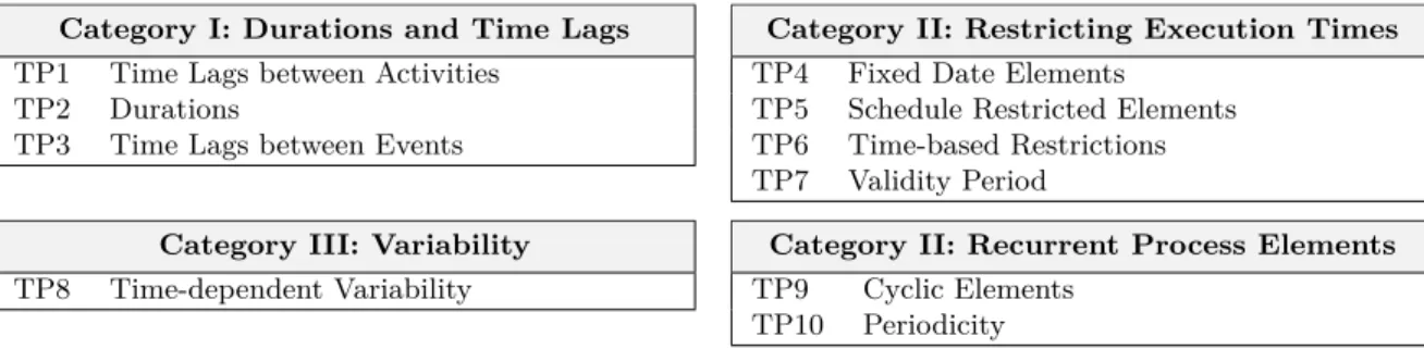
Category I: Durations and Time Lags TP1 Time Lags between Activities
TP2 Durations
TP3 Time Lags between Events
Category II: Restricting Execution Times TP4 Fixed Date Elements
TP5 Schedule Restricted Elements TP6 Time-based Restrictions TP7 Validity Period
Category III: Variability TP8 Time-dependent Variability
Category II: Recurrent Process Elements TP9 Cyclic Elements
TP10 Periodicity Table 1: Process time pattern catalogue [18]
happening during process execution. We assume that activity instances are executed according to the activity life cycle depicted in Fig. 3.When starting a process instance, its activities are in stateNot Activated. As soon as a particular activity becomes enabled, it enters stateActivated. When a user starts an activated activity instance it enters stateStarted and a correspondingstart eventis created. As soon as the user completes the activity instance, its state switches toCompleted and anend event is generated. Finally, non-executed activities (e.g., activities in a non-selected path of an XOR-split) enter stateSkipped.
2.2. Process Time Patterns
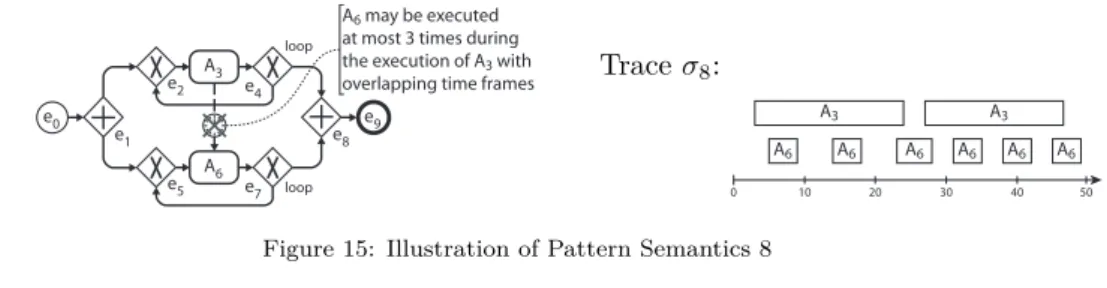
Process Time Patterns (TP) represent temporal constraints commonly occurring in PAISs (cf. Fig. 1) [17, 18]. The 10 time patterns can be divided into 4 distinct categories, based on their implications (cf.
Fig. 1). Pattern Category I (Durations and Time Lags) provides support for expressingdurationsof process elements at different levels of granularity, i.e., activities, activity sets, processes, or sets of process instances.
Furthermore, this category coverstime lags between activities or—more generally—between process events (e.g., milestones). Pattern Category II (Restricting Execution Times) allows specifying constraints regarding possible execution times of single activities or an entire process (e.g., deadlines). Category III (Variability) provides support for expressingtime-based variability during process execution (e.g., varying control-flow depending on temporal aspects). Finally,Category IV (Recurrent Process Elements) comprises patterns for expressing temporal constraints in connection with recurrent activities or process fragments (e.g., cyclic flows and periodicity). Example 2 introduces a simple process along which we will illustrate selected time patterns.
A basic understanding of these patterns is required to understand the formalization provided in Sect. 4.
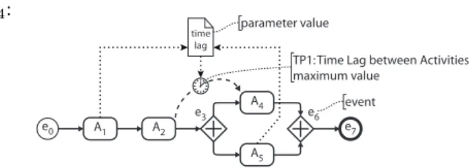
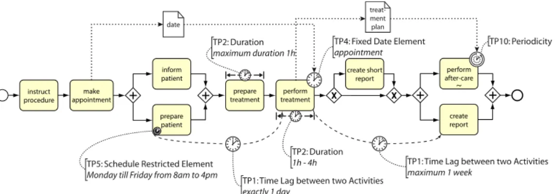
Example 2 (Patient Treatment Process). Consider the simplified patient treatment process depicted in Fig. 4.1 First, a doctor orders a medical procedure for a patient. Then, the responsible nurse makes an appointment with the medical department the treatment will take place in. Before that, the patient needs to be informed about the procedure and be prepared for it. Just before the treatment starts, a specific preparation is required. In turn, after completing the treatment, the doctor creates a short report (if requested). Finally, aftercare is provided and the doctor creates a final medical report, which is then added to the patient record.
When considering the temporal perspective of this business process, a number of temporal constraints can be observed. Example 3 relates these temporal constraints to the time patterns of Fig. 1.
1Note that we use an extension of BPMN to visualize time patterns in process schemas (see [18] for details).
instruct
procedure make
appointment
inform patient
prepare patient
perform after-care
~
create report perform
treatment prepare
treatment
create short report TP2: Duration
maximum duration 1h
TP4: Fixed Date Element appointment
TP1: Time Lag between two Activities maximum 1 week
TP1: Time Lag between two Activities exactly 1 day
TP10: Periodicity
TP5: Schedule Restricted Element Monday till Friday from 8am to 4pm
TP2: Duration 1h - 4h date
treat- ment plan
Figure 4: Simplified treatment process with temporal constraints
Example 3 (Temporal Constraints). Reconsider Fig. 4. Theappointment of thetreatment, made in the context of activitymake appointment, must be met during process execution. This constitutes a Fixed Date Element (TP4), restricting the earliest start date of activity perform treatment. In particular, the respective date will be set during run-time by activitymake appointmentand be stored in data object date. Moreover, this constraint affects the scheduling of preceding activities as well; e.g., the patient needs to be preparedexactly 1 day beforethe treatmenttakes place. This represents aTime Lag between two Activities(TP1) between the start of prepare patientand that of perform treatment. Hence,prepare patient needs to be scheduled in accordance with the appointment of the treatment. Additionally, the preparationof the patient may only be performed during opening hours of the anesthetics department, i.e., fromMonday till Friday between 8am and 4pm. In turn, this represents aSchedule Restricted Element (TP5). It further restricts possible execution times ofprepare patient and hence those of thetreatment itself. Next, due to a high utilization of the treatment room, the preparationof the treatment should not take more than 1 hour; otherwise, the treatmentmight be delayed. This represents a maximumDuration (TP2) for activity prepare treatment. In turn, the treatment itself may take between 1 and 4 hours, which represents a minimum as well as a maximumDuration (TP2), i.e., an interval. Finally, during the execution of activityperform aftercare, different drugs are given to the patient, according to a treatment plandefined by activity perform treatment. Such a treatment plan may state, for example, that drug A must be administeredevery day at 8 am, 1 pm, and 6 pm, and drug Bevery two hours, except when drug A is administered within the same hour. This plan represents a Periodicity(TP10); more precisely, it constitutes the underlying periodicity rule of thePeriodicity represented by activityperform aftercare.
Example 3 demonstrates the diversity and complexity of the temporal perspective of business processes. It further emphasizes the need for precise and formal semantics of the different time patterns. For example, consider the Fixed Date Element of activity perform treatment in combination with theTime Lag be- tween activitiesprepare patientandperform treatment and theSchedule Restricted Elementof activity prepare patient. When combining these three temporal constraints, one may deduce that the treatment itself may only be performed fromTuesday to Saturday. In turn, this restriction needs to be considered when arranging the appointment for thetreatmentduring activitymake appointment. As a prerequisite for determining such implicit restrictions, aprecise formal semanticsneeds to be defined for each time pattern.
Only then, algorithms for automatically detecting such complex interdependencies can be developed. As another example, assume that in certain cases it becomes necessary to reschedule the appointment of activity perform treatmentwhen informing the patient(e.g., due to an overbooking of the treatment room).
For this case, a write access of activityinform patientto data objectdatemust be added, which allows this activity to modify theappointmentfor theFixed Date Elementof activityperform treatment. However, when changing thisappointment, it is not fully clear how to treat activity prepare patient. In particular, the latter must be executedexactly one dayprior to activity perform treatment. As a result, if inform patientis executed after activityprepare patient, it must be decided whether or not the process instance may be continued as is. Particularly, it must be determined whether thetreatmentshall be rescheduled
Pattern Identification
Pattern Validation
Definition of Pattern Semantics
Refinement & Assessment of Pattern Semantics Systematic
Literature Review Data
Sources
Academic Approaches
Lanz et. al (2012) This paper
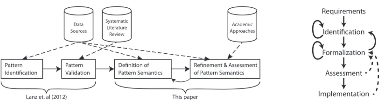
Figure 5: Overall research method
Requirements Identification Formalization Assessment Implementation
Figure 6: Applied research method
within the same day (i.e., theTime Lagbetweenprepare patientandperform treatmentis still satisfied) or thepreparationof the patient must be redone in accordance with the newappointmentfor thetreatment.
Again, such questions can be only be addressed by the PAIS based on precise and formal semantics of the time patterns.
As illustrated by Example 3, there exist numerous variants of the time patterns. To cope with this variability and to keep the number of patterns manageable,design choices(DC) allow for their parametriza- tion [17, 18]. For example, whether a time lag represents a minimum value, maximum value or both (i.e., an interval) constitutes a design choice of theTime Lags between Activitiespattern (TP1). We denote a specific combination of design choices of a time pattern as apattern variant. Usually, PAISs only support a subset of the design choices (i.e., variants) of a particular pattern. However, note that each pattern variant has a slightly different semantics. For example, to be able to exactly define the semantics of patternDuration (TP2), we must specify whether the duration corresponds to a minimum value, a maximum value or both,
i.e., the semantics of TP2 depends on the actual pattern variant.
Finally, when applying a specific pattern variant to a process schema, the restriction represented by the pattern occurrences needs to be determined. In particular, a pattern variant only represents the type of restriction, whereas the restriction itself is configured when applying the pattern to a process schema. When applying patternDuration (TP2) to an activity, for example, the duration restriction needs to be specified, e.g., “maximum duration: 1 hour” for activity prepare treatmentin Example 3. Likewise, it needs to be defined how the particularappointmentrequired in the context of patternFixed Date Element for activity perform treatmentshall be determined at run-time (cf. Example 3). For this purpose,parameter values allow determining the specific temporal constraint represented by a pattern occurrence. Respective parameter values may either be set at build-time (i.e., all process instances share the same value) or at run-time when creating or executing process instances. In the latter case, the parameter value is stored in a data object of the process instance, which will be written either when creating the process instance or executing one of its activities (e.g., data objectdate in Fig. 4). The stored data value is then evaluated by the corresponding pattern instance at run-time. For this purpose, a pattern occurrence may be linked to a data object. In Fig. 4, for example, theFixed Date Element (cf. activityperform treatment) is linked to data objectdate.
3. Research Method
This section describes the research method we applied to develop the formal semantics for the time patterns. This includes the initial identification of the time patterns [18] as well as the definition of their semantics (cf. Fig. 5). We further describe essential requirements for defining a pattern semantics and present the procedure applied for their elicitation.
3.1. Initial Pattern Identification & Validation
Selected time patterns were first introduced in [17]. In turn, [18] provided an informal description of all time patterns as well as empirical evidence for them. Selection criteria were “patterns covering temporal aspects relevant for the modeling and control of business processes and activities, respectively” [18]. Other
Healthcare Domain (Women’s Hospital) [25, 26] 88 processes Healthcare Domain (Internal Medicine) [27, 28, 29] 93 processes
Automotive Domain [30, 31] 55 processes
On-demand Air Service [32, 33] 2 processes
Airline Catering Services [34] 1 process
Transportation [35] 9 processes
Software Engineering [36] 10 processes
Event Marketinga 1 process
Financial Servicea 10 processes
Municipality Processes [37] 4 processes
Student Administrationa 73 processes
Software Asset Managementa [38] 56 processes Build-to-Order Machine Manufacturera 37 processes Total: 439 processes
a Due to copyright & secrecy restrictions some of these pro- cesses cannot be made publicly available.
Table 2: Data sources [18]
process aspects (e.g., data flow) or time support features (e.g., escalation management, verification) were not considered and are thus outside the scope of this paper.
To create a solid basis for the time patterns, first of all, a candidate pattern list was created based on the knowledge and experiences of the authors in the field. Furthermore,design choiceswere introduced for parameterizing the patterns to keep their number manageable. Then, large sets of industrial cases, process schemas, and process documentation were analyzed (cf. Table 2) to provide empirical evidence for each time pattern and to refine the pattern list. Finally, this resulted in a set of 10 time patterns [18]. To validate them and to assess their relevance and completeness, additionally, we conducted a systematic literature review [18].
Finally, existing approaches and tools were evaluated regarding the support of the time patterns.
3.2. Pattern Semantics: Requirements, Procedure & Verification
This section describes essential requirements for defining formal time pattern semantics, the procedure we applied for identifying pattern semantics, and the overall evaluation process chosen. In this context, we follow a design science approach as proposed by Hevner et al. [23, 24] which is outlined in Fig. 6.
Requirements. To be useful for engineers as well as researchers, formal pattern semantics should be as generic as possible, while at the same time being as specific as necessary to avoid ambiguities (R1). In particular, if formal pattern semantics are too restrictive, they will not be applicable in many practically relevant cases.
Conversely, if it is too permissive, it may allow for too many ambiguities and hence be of limited benefit (especially when trying to detect inconsistencies). Furthermore, formal pattern semantics must consider all pattern variants that may be configured based on different combinations of design choices (R2). To ensure that different implementations of a particular pattern share the same underlying semantics, its formal semantics needs to precisely define the effects, the respective pattern shall have on process enactment, as well as its interactions with different elements of the control flow perspective (R3). For the same reason, the impact, process instance data has on pattern semantics, needs to be specified (R4). Finally, as emphasized, any pattern semantics will only be useful for PAIS engineers if it is independent of a particular process modeling language (e.g., BPMN vs. EPC) or process modeling paradigm (e.g., imperative vs. declarative) (R5).
Identification. To identify the semantics of each time pattern, we first analyze the data sources used for pattern identification as well as three additional sources (cf. Table 2). Note that most data sources were gathered by us over the last decade. Moreover, in most cases we were involved in the elicitation of the processes (e.g., interviews with domain experts). In all these cases, we paid attention to thoroughly and completely record respective processes. We not only described the control flow, data flow, and organizational perspectives, but also documented additional requirements and business rules like exceptional cases, exception
handling rules, compliance rules, and temporal constraints along with the processes. Moreover, we ensured that these additional requirements are accurately described including their intended purpose and effects as declared by domain experts. This enables us to use the data sources to analyze the intended semantics of each pattern occurrence. Next, for each time pattern, we combine the collected semantics of all its occurrences–considering the respective pattern variant–to derive the overall semantics of the pattern. Finally, if appropriate, we remove unnecessary restrictions from the overall pattern semantics.
Formalization. Workflow patterns have been defined based on languages with an inherent formal semantics (e.g., pi-calculus [39]). However, such formalisms cannot be used to define the semantics of time patterns without significant extensions since they do not consider the temporal perspective. Beyond that, different techniques, commonly used for describing the temporal properties of a system, exist. Examples include temporal logics [40], timed Petri nets [41], timed automata [42], and execution traces [21]. Basically, all these techniques can be used for describing the formal semantics of time patterns.
On one hand, the definitions of the formal semantics should be independent of a particular process modeling language or paradigm. On the other, they should be closely related to the execution semantics of processes. To cope with this trade-off, this paper usesexecution traces as basis for formalizing pattern semantics. Anexecution trace represents a possible execution of a process schema in terms of all events that occurred during the execution of the respective process instance together with their time stamps (cf.
Sect. 4.1). Based on this, we can specify which execution traces (i.e., process instances) arevalid according to the time patterns found in the respective process schema. Thus, we obtain an approach that is independent of the particular process modeling language and paradigm; yet, we are still able to precisely define pattern semantics. By associating the defined pattern semantics with a process meta model, the effects a particular pattern has on process enactment, as well as its interactions with different elements of the meta model, can be derived in a precise and formal way.
Taking the definition of the formal semantics we reconsider each pattern occurrence observed in any data source (cf. Table 2), and compare the described semantics with the formal definitions; i.e., we revisit theIdentification step (cf. Fig. 6). If the semantics of one of the pattern occurrences in the data sources is not precise enough, we discuss it with the co-authors not involved in the identification of this particular occurrence. Whenever necessary, we discuss a pattern occurrence with the respective stakeholder involved in the initial elicitation of the data source to ensure that the pattern semantics meets the one the domain experts had in mind. If the formal semantics of a particular time pattern needs to be modified, we implement the required change (i.e., we repeat stepsIdentificationandFormalization). We repeat these steps until all occurrences of every pattern observed in any data source are covered by the formal pattern semantics. This ensures that the formal semantics indeed cover all pattern occurrences in the data sources.
Implementation and Testing. In a final step, we use the formal semantics of the time patterns as foundation for implementing selected time pattern variants in the ATAPIS Toolset [43]. With this toolset we aim to provide a comprehensive framework enabling the specification, enactment and monitoring of processes with temporal constraints in PAISs. Moreover, we are currently expanding this implementation such that it may serve as a reference implementation for the time patterns. We further use it to once more test that the formal descriptions accurately describe the semantics of the time patterns. For the latter purpose, we model several processes from the data sources using the ATAPIS Toolset. For each of the resulting process schemas, we then use ATAPIS to simulate the execution of multiple process instances. Finally, for each pattern occurrence and for each of the simulated process instances we compare the resulting execution log with the expected results and the formal semantics of the time patterns. This shows that both the formal semantics of the time patterns and their implementation work as intended.
4. On the Formal Semantics of Time Patterns
Sect. 4.1 first defines basic notions (e.g., event andtrace) used throughout this paper. Sect. 4.2 then provides the formal semantics of each time pattern.
S2:
A1
A3
A5
A4
A6
Activity End Event Activity Start Event e0
e9
e2 e7
e10
e8 eA
1S eA
1E
eA
3S eA
3E eA
4S eA
4E
eA
5S eA
5E eA
6S eA
6I eA
6E
Process End Event External Event
Process Event Process Start Event
Milestone Event
Intermediate Activity Event Figure 7: Events occurring during a process
4.1. Temporal Execution Traces
We use the notion ofeventas a general term for something that happens during the execution of a process instance, e.g., the start and end of an activity, executed in the context of a particular process instance, constitute such events (cf. Fig. 7). External events (e.g., reaching a milestone or receiving a message) may exist as well. Finally, intermediate events may be triggered inside a long-running activity (cf. Fig. 7).
Definition 1 (Event, Event occurrence). LetPS be the set of all process schemas and E be the set of all events. Then: The set of all events that may occur during the execution of an instanceI of process schema S∈ PS is denoted asES ⊆ E. (Note that, without loss of generality, we assume unique labeling of events.) Let further C be the total set of absolute time points. Then:
ϕ= (e, t)∈ E × C
denotes the occurrence of evente∈ E at time pointt∈ C, i.e.,tdefines the exact point in time at which event eoccurred. Moreover, ΦS⊆ ES× C denotes the set of all possible event occurrences during the execution of process schemaS. Finally, for the sake of brevity, we use notionsϕe andϕt when referring to evente or
time stamptof an event occurrence ϕ= (e, t). ♦
Based on events and event occurrences, we define the notion oftemporal execution trace(tracefor short) which is inspired by [21]. We assume that all events related to the execution of a process instance are recorded in a temporal execution trace together with a time stamp designating their time of occurrence.Formally:
Definition 2 (Temporal Execution Trace). LetPSbe the set of all process schemas. Then: For schema S∈ PS,QS denotes the set of all temporal execution traces producible onS. LetΦS be the set of all event occurrences that may occur during the execution ofS andϕ= (e, t)∈ΦS denote the occurrence of eventeat time pointt. A temporal execution traceσS ∈ QS is defined as ordered set of event occurrencesϕi:
σS =hϕ1, . . . , ϕni, ϕi∈ΦS, i= 1, . . . , n, n∈N
Without loss of generality, we assume that events inσS do not occur at exactly the same point in time. ♦ Note that we consider events to be instantaneous. Thus—with sufficient clock precision—one may assume that there are no events of a trace occurring at exactly the same time. We make this assumption to foster comprehensibility of the pattern semantics and to reduce ambiguities. However, it does not constitute a restriction of the presented semantics, and may be dropped without having to change pattern semantics.
In the latter case, however, it might not always be clear which event exactly violates a particular pattern occurrence (i.e., there might be multiple equivalent reasons for the violation of a pattern occurrence).
Since the pattern semantics are defined based on events and event occurrences, we define nodes, activities, and gateways based on events. Remember that nodes may represent both activities and gateways (cf.
Sect. 2.1). Respective definitions are based on the events that may occur during the execution of the particular node. Since gateways (e.g., XOR-splits, AND-joins) merely serve structuring purposes, without loss of generality, we may assume that the processing of a gateway does not take any time during process
execution. If a gateway consumes time during its execution (e.g., evaluating an XOR decision), this may simply be represented by an activity directly preceding the gateway. Note that, this is no particular restriction of the presented pattern semantics, but only serves the purpose of simplifying some of the formulas.
Definition 3 (Node, Activity, and Gateway). Let PS be the set of all process schemas andNS ⊂2ES be the set of all nodes process schemaS∈ PS refers to.
A noden∈ NS is defined as unique, non-empty set of events n⊂ ES (i.e., ∀n∈ NS :n6=∅). Thereby, the sets of events of all nodes belonging toS are disjoint: ∀n, m∈ NS, n6=m:n∩m=∅. An occurrence of a nodenin a temporal execution traceσS is marked by the occurrence of at least one of the respective events, i.e.,∃e∈n,∃t∈ C :ϕe= (e, t)∈σS. In turn, an activity is a special kind of node with a single start and single end event (cf. Sect. 2.1). Let AS⊆ NS be the total set of activities S refers to. An activitya∈ AS
contains (at least) a unique start eventeaS and a unique end eventeaE, i.e.,
∀a∈ AS :∃eaS, eaE∈ ES :{eaS, eaE} ⊆a
An occurrence of an activityais marked by the occurrence of at least both the start event eaS and the end eventeaE in trace σS, i.e., ∃t1, t2∈ C:ϕaS = (eaS, t1)∈σS∧ϕaE = (eaE, t2)∈σS.
Finally, a gatewayis a special kind of node represented by single eventedenoting the time the gateway is processed by the system, i.e., for a gatewayc∈ NS it holds|c|= 1. ♦
Example 4 illustrates these definitions.
Example 4 (Temporal Execution Trace). Consider Fig. 7. An example of a temporal execution trace on process schemaS2 may be as follows:2
σ=h(e0,2),(eA1S,5),(eA1E,10),(e2,11),(eA5S,15),(eA5E,18), (e10,19),(eA6S,30),(eA6I,32),(eA6E,37),(e7,38),(e8,39)i
This trace indicates that the corresponding process instance was started (i.e.,e0) at time 2. At time 5, activity A1 was started (eA1S). In turn, A1 was completed at time 10 (eA1E); i.e., A1 had duration10−5 = 5. Next, evente2 occurred at time 11 and the lower path was chosen, which is indicated by the occurrence of start eventeA5S related to activityA5. Remember that none of the events of the upper path occurs within the trace as the respective path had been skipped. Further note that the occurrence of XOR-splite2 is indicated by a single event, i.e., processing of the gateway does not take any time. After completing activity A5 (eA5E), milestone evente10 was triggered. Next,A6 was started at time 30. Furthermore, during the execution ofA6, the intermediate activity eventeA6I was triggered. Finally, after completion of A6, events e7 ande8 were triggered completing the process instance.
When defining the semantics of the time patterns, for some of them the iteration of a loop structure needs to be taken into account.
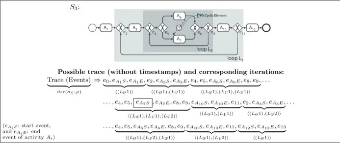
Example 5 (Cyclic Elements). Consider process schemaS3in the upper part of Fig. 8. It comprises two nested loops. Thereby, the inner loop L2 contains two alternative branches either executing activityA6 or A7. As indicated in Fig. 8, the time lag betweenA6 andA7 must be a Cyclic Element (TP9) since A6 and A7 cannot be executed within the same iteration of the respective loop. In turn, time pattern TP9 requires the target activity to be contained in an iteration succeeding the one to which the source activity belongs to.
Assume that the cyclic element only restricts the maximum time lag between directly succeeding iterations (Design Choice K[a]), i.e., the respective maximum time lag must be obeyed solely ifA7 is executed in an iteration of Loop L2 directly afterA6 without executing another instance of A6,A7 orA10 in between. To formalize this semantics, it is not sufficient to introduce an iteration counter for activities. Regarding Fig. 8 it cannot always be detected whether another iteration ofL1 has been executed between the two instances of A6 andA7. Hence, the current iteration of the outer loopL1 must be considered as well.
2In the following, without loss of generality, we use integers starting at 0 for representing absolute time pointsc∈ C.
S3:
A1 e2
e0 A3
A6
A7
e4 e9 A10
e11 A12 e13
e5 e8
loop L1 loop L2
TP9: Cyclic Element
Possible trace (without timestamps) and corresponding iterations:
Trace (Events)
| {z }
iter(σS,ϕ)
⇒e0, eA1S, eA1E,
| {z }
h(L0:1)i
e2, eA3S, eA3E,
| {z }
h(L0:1),(L1:1)i
e4, e5, eA6S, eA6E, e8, e9,
| {z }
h(L0:1),(L1:1),(L2:1)i
. . .
. . . , e4, e5, eA7S , eA7E, e8, e9,
| {z }
h(L0:1),(L1:1),(L2:2)i
eA10S, eA10E, e11,
| {z }
h(L0:1),(L1:1)i
e2, eA3S, eA3E,
| {z }
h(L0:1),(L1:2)i
. . .
. . . , e4, e5, eA6S, eA6E, e8, e9,
| {z }
h(L0:1),(L1:2),(L2:1)i
eA10S, eA10E, e11,
| {z }
h(L0:1),(L1:2)i
eA12S, eA12E, e13
| {z }
h(L0:1)i (eAiS: start event,
andeAiE: end event of activityAi)
Figure 8: Nested loops and iterations
Generally, one must always consider the iteration of the inner-most loop in respect to the iteration of any surrounding loop. Regarding process schemaS3 in Fig. 8, for example, an instance of activityA6 may belong to the 3rd iteration of loopL2within the 2nd iteration of loopL1.
For the sake of simplicity and to be able to uniquely identify the iteration of each activity, we presume well-nested loops (see Fig. 8). If a process schema is not well-nested, in most practically relevant cases, we can transform it into a behaviour-equivalent, well-nested representation [44, 45, 46]. Nevertheless, we are aware that this might not be possible for all non-well-nested schemas [44]. Consequently, the notion of (loop) iteration is defined as follows:
Definition 4 (Iteration). LetS ∈ PS be a process schema. Then: A loopL is a process fragment (i.e., L⊆ ES) with a Loop-Start as entry node and a corresponding Loop-End as exit node. The set of possible iterations ofS is given by IS ⊆22ES×N. Accordingly, the iteration of a loop is defined as ordered set
I=h(L0:nL0), . . . ,(Lk:nLk)i ∈ IS
I uniquely identifies each loop and its current iteration with respect to the iteration of any surrounding loop.
Thereby, L0 is the given process schema andLi (1≤i≤k) thei-th loop structure. In turn, nLi (1≤i≤k) designates the iteration count of loopLi with respect to its directly surrounding loop Li−1.
Function iter(σS, ϕ)returns the current iteration of the inner-most loop surrounding eventϕe. Formally:
iter:QS×ΦS7→ IS with iter(σS, ϕ) =h(L0:nL0), . . . ,(Lk:nLk)i
andL1, . . . , Lk being the loop structures surrounding eventϕe. ♦
Example 6 (Iteration). Consider Fig. 8: Below process schemaS3, a temporal execution trace is shown.
Moreover, for each event in the trace, the value of iter(σS, ϕ)is given; e.g., regarding the occurrence of event eA7S during the 2nd iteration of loopL2 within the 1st iteration of loop L1, we obtain
iter(σS,(eA7S,·)) =h(L0: 1),(L1: 1),(L2: 2)i This is indicated in the second line of the execution trace depicted in Fig. 8.
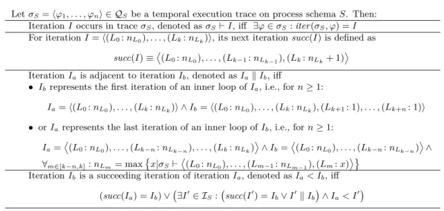
Based on Def. 4, Table 3 summarizes useful notions that will facilitate the following formalization of the time patterns. Functionsucc(I) determines the next iteration after iterationI. In turn, the adjacency
LetσS=hϕ1, . . . , ϕni ∈ QS be a temporal execution trace on process schemaS. Then:
IterationIoccurs in traceσS, denoted asσS`I, iff ∃ϕ∈σS:iter(σS, ϕ) =I For iterationI=h(L0:nL0), . . . ,(Lk:nLk)i, its next iterationsucc(I) is defined as
succ(I)≡
(L0:nL0), . . . ,(Lk−1:nLk−1),(Lk:nLk+ 1) IterationIais adjacent to iterationIb, denoted asIakIb, iff
• Ibrepresents the first iteration of an inner loop ofIa, i.e., forn≥1:
Ia=h(L0:nL0), . . . ,(Lk:nLk)i ∧Ib=h(L0:nL0), . . . ,(Lk:nLk),(Lk+1: 1), . . . ,(Lk+n: 1)i
• orIarepresents the last iteration of an inner loop ofIb, i.e., forn≥1:
Ia=
(L0:nL0), . . . ,(Lk−n:nLk−n), . . . ,(Lk:nLk)
∧Ib=
(L0:nL0), . . . ,(Lk−n:nLk−n)
∧
∀m∈[k−n,k]:nLm = max
x|σS`
(L0:nL0), . . . ,(Lm−1:nLm−1),(Lm:x) IterationIbis a succeeding iteration of iterationIa, denoted asIa< Ib, iff
(succ(Ia) =Ib)∨ ∃I0∈ IS: succ(I0) =Ib∨I0kIb
∧Ia< I0
Table 3: Useful notions
operatorkallows determining adjacent iterations–two iterations are adjacent if one of them is the first or last iteration of a nested loop with respect to the other iteration. Finally, the<-operator determines whether the second iteration is (transitively) succeeding the first one.
Since a particular event may occur multiple times within a trace (e.g., at the presence loops), we further define functionoccur(σS, e). It returns all event occurrences of an eventewithin a trace:
Definition 5 (Trace Occurrences). Let S ∈ PS be a process schema and σS be a trace on S. Then:
occur(σS, e)corresponds to a function returning all occurrencesϕ= (e,·)of evente∈ ES withinσS. Formally:
occur :QS× ES 7→2ΦS with occur(σS, e) ={ϕ|∃t∈ C:ϕ= (e, t)∈σS}
♦
Def. 5 implies thatoccur(σS, e) =∅holds, if@t∈ C: (e, t)∈σS, e.g., in case the respective path has been skipped (cf. Example 4).
Similar to events, activities may occur multiple times within a trace. In turn, each instance of an activity is marked by the occurrence of its start and end event (cf. Def. 3). For this purpose, we introduce function occur(σS, a), which returns all instances of a particular activity a(i.e., occurrences of the start and end events) within a trace:
Definition 6 (Activity Occurrence). Let S ∈ PS be a process schema and σS be a trace on S. Then:
occur(σS, a) returns all occurrences (ϕS, ϕE)of the start and end event eaS, eaE ∈ ES of activitya∈ AS (i.e., {eaS, eaE} ⊆a) within traceσS.Thereby, two occurrences of events eaS and eaE belong to the same activity instance if they occur within the same iteration. Formally:
occur :QS× AS 7→2ΦS×ΦS with occur(σS, a) ={(ϕS, ϕE)∈ΦS×ΦS |
ϕS ∈occur(σS, eaS)∧ϕE∈occur(σS, eaE)∧iter(σS, ϕS) =iter(σS, ϕE)}
Note that the start eventeaS of an activity instance always occurs before the corresponding end event eaE,
i.e.,∀(ϕS, ϕE)∈occur(σS, a) :ϕtS< ϕtE ♦
For the sake of readability, we will omit subscript S in the formulas if the respective process schema becomes evident from the given context.
S4:
A1 A2
e0 e7
A4
A5
e3 e6
time lag
TP1: Time Lag between Activities maximum value
parameter value
event
Figure 9: Run-time parameter value and concurrent change
4.2. Time Pattern Semantics
The semantics of the time patterns can now be defined by characterizing the temporal execution traces σS that may be produced by instances of a process schemaS. In particular, we specify which temporal execution traces satisfy the temporal constraints expressed by any time pattern applied toS. Formally:
Definition 7 (Temporal Compliance). A temporal execution trace σS ∈ QS is temporally compliant with the set of temporal constraints defined on process schema S ∈ PS if and only if σS is temporally compliant with each of the temporal constraints corresponding toS. In this context, temporal compliance of a trace with a particular temporal constraint onS is defined by the semantics of the respective time pattern. ♦ Based on Defs 1-7, we are able to describe the formal semantics of all time patterns. Thereby, we do not consider at which point in time the parameter values of a pattern occurrence are set (i.e., at build-time, process creation-time, or run-time; Design Choice A) as this does not affect formal pattern semantics.
However, we consider which parameter value shall be valid in the context of a particular pattern instance;
i.e., if the parameter value of a pattern occurrence may be modified during run-time (e.g., deadlines may be changed), we specify which of the values shall be relevant for a particular instance of a pattern occurrence when defining pattern semantics.
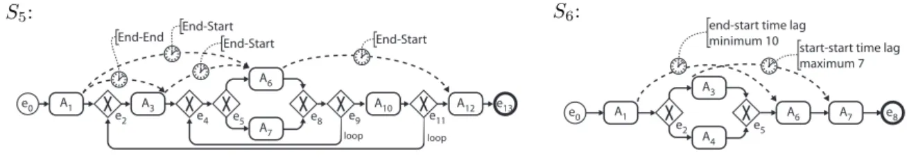
Example 7 (Run-time Parameter Values). Consider process schemaS4 in Fig. 9: S4 contains a maxi- mum time lag between activitiesA2and A4. The value of the time lag is provided by data objecttime lagat run-time. In turn, this data object is written twice during process execution by activitiesA1 and A5. Note thatA5 may be executed (or—more important—be completed) either before, during, or after executingA4. Depending on the completion time of A5, the time lag may use a different version of the parameter value, i.e., a different version of the value of data objecttime lag. Therefore, it is important to precisely state which of these versions shall be valid for a particular instance of the time lag.
To structure our formalization effects, we bundle time patterns with similar or related foundations as they have same or similar formalization.
The first set of time patterns with similar foundations comprises patterns TP1 (Time Lags between two Activities), TP2 (Duration), TP3 (Time Lags between Arbitrary Events), and TP9 (Cyclic Elements). These patterns restrict the relative time distance between pairs of events that may occur during the execution of a process instance. The kind of relative time distance expressed constitutes a pattern-specific design choice (Design Choice D); i.e., the time distance may be a minimum value, a maximum value, or an interval. The kind of events to which a specific pattern can be applied may be restricted by the pattern itself; e.g., a time lag between activities may only be applied to the start or end events of two activities. Furthermore, only pairs of event occurrences, whose iterations are consistent with the pattern, may be considered; e.g., for an activityDuration(TP2;Design Choice C[a]), the occurrences of the start and end event of the respective activity must belong to the same iteration.
Definition 8 (Relative time distance between events). LetC be the total set of absolute time points andDbe the set of relative time distances. Let eX andeY represent the source and target events related to the time distance, i.e., the events for which the time distance is specified. Temporal compliance of a given traceσ with a relative time distance between eventseX andeY is then defined as follows:
![Table 2: Data sources [18]](https://thumb-eu.123doks.com/thumbv2/1library_info/5208855.1668776/7.892.140.559.163.406/table-data-sources.webp)