A Microeconomic Explanation of the EPK Paradox

SFB 649 Discussion Paper 2009-010

A Microeconomic

Explanation of the EPK Paradox

Wolfgang Härdle*

Volker Krätschmer**

Rouslan Moro***

*Humboldt-Universität zu Berlin, Germany

**Technische Universität Berlin, Germany

***DIW Berlin, Germany

This research was supported by the Deutsche

Forschungsgemeinschaft through the SFB 649 "Economic Risk".

http://sfb649.wiwi.hu-berlin.de ISSN 1860-5664

S FB

6 4 9

E C O N O M I C

R I S K

B E R L I N

A Microeconomic Explanation of the EPK Paradox ^∗

Wolfgang K. H¨ ardle

, Volker Kr¨ atschmer

, Rouslan A. Moro

.

Abstract

Supported by several recent investigations the empirical pricing kernel paradox might be considered as a stylized fact. In Chabi-Yo et al. (2008) simulation studies have been presented which suggest that this paradox might be caused by regime switching of stock prices in financial markets. Alternatively, we want to emphasize a microeconomic view. Based on an economic model with state dependent utilities for the financial investors we succeed in explaining the paradox by changes of the risk attitudes. Theoretically, the change behaviour is compressed by the pricing kernels. As a starting point for empirical insights we shall develop and investigate inverse problems in terms of data fits for estimated basic values of the pricing kernel.

Keywords: Pricing kernel, representative agent, empirical pricing kernel, epk paradox, state dependent utilities, switching points. JEL Classification: D01, D58, C02, G13

AMS Classification: 15A29, 62G07, 62G35

∗This research was supported by Deutsche Forschungsgemeinschaft through the SFB 649 “Economic Risk”.

†Center for Applied Statistics and Economics, Humboldt-Universit¨at zu Berlin, Spandauer Str. 1, 10178 Berlin;

e-mail: haerdle@wiwi.hu-berlin.de.

‡Center for Applied Statistics and Economics, Humboldt-Universit¨at zu Berlin, Spandauer Str. 1, 10178 Berlin and Institute of Mathematics, Berlin University of Technology, 10623 Berlin; e-mail: kraetsch@math.tu-berlin.de.

§Center for Applied Statistics and Economics, Humboldt-Universit¨at zu Berlin, Spandauer Str. 1, 10178 Berlin and German Institute for Economic Research (DIW Berlin), Mohrenstr. 58, 10117 Berlin; e-mail: moro@diw.de.

1 Introduction

The empirical pricing kernel paradox refers to the empirical phenomenon that the observable behaviour of investors in financial markets conflicts with the traditional expected utility framework. Several recent studies support the conjecture that this deviation evolves into a stylized fact. All the investigations are settled within similar economic models assuming representative agents in financial markets whose indirect preferences have classical expected utility representation. Additionally, the risk neutral valuation principle is supposed to be valid for the financial markets by means of pricing kernels. If the pricing kernels represent state contingent equilibrium prices they might be identified with the v. Neumann-Morgenstern indices of the representative agents. As a consequence the pricing kernels should be nonincreasing.

In the studies of Ait-Sahalia and Lo (2000), Jackwerth (2000), Detlefsen et al. (2007), Constantinidis et al. (2009) different econometric methods have been applied to estimate pricing kernels with varying underlying models for the financial markets. It turned out as a common result, that the estimates, the so called empirical pricing kernels, have non-monotonic shape regardless of the used data sets. This difference between the theoretical property of the pricing kernel and the observed failure of it is what we shall call the empirical pricing kernel paradox. A further confirmation of it is provided by Golubev et al. (2008). In this paper a test for monotonicity of pricing kernels has been introduced, and applied to DAX data over several periods. Typically, the nullhypothesis that the pricing kernel is nonincreasing was rejected.

More recently, simulation studies in Chabi-Yo et al. (2008) suggest to explain by regime switches of the prices for the underlyings of the financial markets. Since it is plausible to view regime switches as consequences of changes in the investor’ risk attitude, we want to emphasize a microeconomic perspective.

The aim is to provide an extended economic model, which allows non-monotone pricing kernels. The crucial idea is to propose financial investors whose risk attidudes might be sensible to the prices in the financial markets. More technically, we shall assume state dependent utilities to represent the preferences of the financial investors.

The paper is organized as follows. In section2 we shall introduce our model for the financial market.

Also the classical relationship between the utilities of representative agent and the pricing kernel will be reviewed. Afterwards, the problem to estimate pricing kernel will be considered. Afterwards we shall point out the empirical pricing kernel paradox. A simple consumption model based on state dependent utilities

for the investors will be introduced in section 3. Within this framework we shall retain the relationship between preferences of investors and pricing in the market by an analogous result. It will turn out that dependent on the stock prices the v. Neumann-Morgenstern utility index for the representative agent might switch between different types of utilities, meaning possible changes of the risk attitudes. In particular pricing kernels might be non-monotone. The switching points and the types of utilities describe local risk attitudes of the investors. So in order to get some insight on the changing of the risk attitudes it might be useful to analyze the switching behaviour of the pricing kernel. The idea is to find a good fit of estimated basic values by given base functions expressing the possible types utilities. Essentially, there are inverse problems behind which will be developed and investigated throughout section 4. Several mathematical results and proofs of quite technical nature have been delegated to appendices A, B, C respectively.

2 Financial Investors’ within the Expected Utility Frame- work and the Empirical Pricing Kernel Paradox

Let [0, T] be the time interval of investment in the financial market, where t= 0 denotes the present time and t=T ∈]0,∞[ the time of maturity.

Furthermore it is assumed that a riskless bond and a risky asset are traded in the financial market as basic underlyings. The price process (B_t)_t∈[0,T] of the riskless bond is defined by

dBt

B_t =rt dt,

via a deterministic Riemannian-integrable interest process (rt)t∈[0,T]. The price process (St)t∈[0,T] of the risky asset is assumed to be a nonnegative semimartingale with constant S₀ and continuously distributed marginals St (t ∈]0, T]). Outstanding examples for such financial markets are the Black-Scholes model, non-parametric diffusion models as in Ait-Sahalia and Lo (2000) and GARCH models. Notice that time discrete models may be subsumed under this setting.

Furthermore let us suppose that the financial market is arbitrage free in the sense that there exists at least one equivalent martingale measure.

We further assume that the risk neutral valuation principle is valid for nonnegative pay offsψ(S_T).That means that there is some unknown Radon-Nikodym densityπ of a martingale measure such that the price

of any ψ(ST) is characterized by E

h e⁻

RT

0 rx dxψ(ST)π i

=E h

e⁻

RT

0 rx dxψ(ST)E[π|S_T] i

. (1)

By factorization we find some Borel-measurable K_π with E[π|S_T] =K_π(ST),so that E

h e⁻

RT

0 rx dxψ(ST)π i

= Z ∞

0

e⁻

RT

0 rx dxψ(x)K_π(x) pS_T(x) dx, (2) where pS_T denotes a density function of the distribution of ST. Equation (2) gives reason to call K_π the pricing kernel (w.r.t. π).

Let us now embed the financial market into an economic model where the investors of the financial market are consumers whose consumptions rely on the price S_T of the stock at maturity only. Within the classical framework, where the investor preferences may be represented by expected utilities, there exists a link between the risk attitude of the investors and the pricing rule of the financial markets. It is built upon the assumption of a representative agent whose indirect utility U({¯e(ST)}), depending on the aggregated market endowment ¯e(S_T), has expected utility representation U(¯e[S_T]) = E[u(S_T)] with concave v. Neumann-Morgenstern utility indexu.Under some further technical conditions on the investor preferences, and the additional specification ¯e(S_T) = S_T

S0

,then there is some positiveβ such that du

dx x=^sT_S

0

=βK_π sT

S0

for almost every realization sT of ST. This relationship might be obtained by using methods as in the sections 6.1, 6.2 of Karatzas and Shreve (1998). For a rigorous formulation and derivation see Corollary A.2 in Appendix A. It should be emphasized that within the classical expected utility framework the pricing kernel has to be nonincreasing due to concavity of the utility index u.

Several recent econometric studies are concerned with the problem to estimate the pricing kernel, calling the estimatorsempirical pricing kernels(EPK) (cf. Ait-Sahalia and Lo (2000), Jackwerth (2000), Detlefsen et al. (2007), Constantinidis et al. (2009)). Typically, we may find a shape of the empirical pricing kernel as visualized in the following graphic which is borrowed from Detlefsen et al. (2007).

The figure shows empirical pricing kernels resulting from different estimation methods. Here estimations of Garch-, Garch-M and discrete Heston models for stock prices had been done. The underlying data are

0.5 1 1.5 2 0

1 2 3 4 5 6 7

return

epk

returns GARCH GARCH in mean

Figure 1: EPK on 24 March 2000. Across data sets, methods, models and markets

same form, the same characteristic features like e.g. the hump, and they differ in absolute terms slightly.

In particular the empirical kernels fail to be monotone, contrasting the classical theory within the expected utility framework. This is what we shall call the empirical pricing kernel paradox.

A further investigation in Detlefsen et al. (2007) based on DAX data in July 2002 and June 2004 confirmed the paradox. Moreover, in the above mentioned studies Ait-Sahalia and Lo (2000), Jackwerth (2000) one may find similar pictures of the empirical pricing kernels. So summarizing, the empirical pricing kernel paradox has been observed across different times independently of the data sets, the markets, the models of stock prices and the employed estimation methods. It is further supported by Golubev et al. (2008), where a statistical test for the monotonicity of pricing kernel has been developed. The application to DAX data over different periods lead to the rejection of the null hypothesis that the pricing kernel is nondecreasing, in almost every case.

3 A Microeconomic View on the EPK Paradox

A first explanation for the empirical pricing kernel paradox has been offered by Chabi-Yo et al. (2008).

The crucial idea of the authors is to suppose that regime switches are inherent of the price process of the stock market. More specifially, within a discrete time period {0,1, ..., T}, there are two types of price processes (S_t⁰)_{t∈{0,...,T}},(S_t¹)_{t∈{0,...,T}} for the risky asset which have joint continuous distributions, and constitute separately together with the riskless bond arbitrage free financial markets in the sense of section 2. Furthermore, Chabi-Yo et al. (2008) assume a latent regime switching variables in terms of an

unobservable Markov-chain (Ut)t∈{0,1,...,T} of Bernoulli-distributed random variables. The observable price process (S_t)t∈{0,1,...,T} is then modelled by S_t =U_tS_t¹+ (1−U_t)S_t⁰ for t ∈ {0, ..., T}. Assuming the risk neutral valuation principle for the latent two basic financial markets and for the observable one, the authors drew a comparison of the associated pricing kernels via a simulation study. Indeed it turned out that the empirical pricing kernels in the separated financial market were nondecreasing whereas the empirical pricing kernel in the integrated financial market failed to have the property of monotonicity. Therefore the empirical pricing kernel might be explained by a switch of the price processes of the underlyings in the financial market.

Referring to Chabi-Yo et al. (2008), we want to stress a microeconomic viewpoint. Based on the initializing thought that regime switching is caused by changes of the investors’ preferences our aim is to make the influence of these changes on the shape of the pricing kernels more explicit. In the following we shall provide a simple economic model underlying the financial market where the pricing kernel need not to be nonincreasing. The key idea is to consider the investors as consumers whose preferences are representable by utilities dependent on the prices of the stock. This refers to the concept of state dependent preferences.

An axiomatic justification is provided by Karni et al. (1983).

Let us assume that we have m consumers who choose among nonnegative random variablesc(S_T).They have exogeneous endowments by initial capitals w₀¹, ..., w^m₀ >0 and state dependent endowement in form of nonnegative random variables e₁(S_T), ..., e_m(S_T). Their individual budget constraints for c(S_T) is therefore:

Z ∞ 0

exp(−

Z T 0

r_y dy)c(x)K_π(x)p_ST(x)dx≤w₀ⁱ+ Z ∞

0

exp(−

Z T 0

r_y dy)e_i(x)K_π(x)p_ST(x)dx, i= 1, . . . , m.

(3) The consumers are assumed to have state dependent utilities in terms of extended expected utility pref- erences within the terminology of Mas-Colell et al. (1995). That means in particular that consumerihas numerical representation of her/his preferences as:

Uⁱ{c(S_T)}=E

exp(−

Z T 0

r_x dx)uⁱ{S_T, c(S_T)}

,

where uⁱ : R+ ×R+ → R∪ {−∞} denotes a state dependent v. Neumann-Morgenstern utility index

satisfying:

uⁱ(x, y)∈Rforx≥0, y >0, (4)

uⁱ(x,·) is strictly increasing and strictly concave for anyx≥0, (5)

uⁱ(·, y) is Borel-measurable for every y≥0. (6)

At time of maturity T the market has an aggregated endowment ¯e(ST)^def=

m

P

i=1

{w₀ⁱ+ei(ST)}. It is assumed that simultaneous consumption is allowed for consumption vectors (c₁(S_T), ..., c_m(S_T)) which satisfy the individual budget constraints and obey the aggregated endowment in the sense of

m

P

i=1

ci(ST)≤¯e(ST).Such vectors are called admissible, and they are gathered by a set say A(see Mas-Colell et al. (1995)).

Next it is supposed that the consumers have chosen their consumptions (¯c₁(S_T), ...,¯c_m(S_T)) such that the following properties are fulfilled.

(ii)individual optimization: For each consumerithe consumption ¯c_i(S_T) solves the optimization problem

maxUⁱ{c(S_T)}, (7)

s.t. c(S_T) satisfies individual budget constraint (3).

(i) market clearing:

m

X

i=1

¯

c_i(S_T) = ¯e(S_T). (8)

The conditions (8) and (8) describe a weak version of a so called contingent Arrow Debreu equilibrium (see Dana and Jeanblanc (2003), sect. 7.1). As a by product (¯c₁(S_T), ...,c¯_m(S_T)) is a Pareto optimum too, i.e. there is no (c1(ST), ..., cm(ST)) ∈ A with Uⁱ{c_i(ST)} ≥ Uⁱ{¯ci(ST)} for every i and such that Uⁱ⁰{c_i0(S_T)} > Uⁱ⁰{¯c_i0(S_T)} for at least one i₀. Therefore, by the so called Negeishi method (cf. Dana and Jeanblanc (2003)) we may find nonnegative weights α1, ..., αm summing to 1 such that

m

X

i=1

α_iUⁱ{¯cⁱ(S_T)}=U_α{¯e(S_T)}^def= max ( _m

X

i=1

α_iUⁱ{c_i(S_T)} |

m

X

i=1

c_i(S_T)≤e(S¯ _T) )

(9) Let u_α:R²+ →R∪ {−∞,∞}be defined by

u_α(x, y) = sup (

exp(−

Z T 0

r_x dx)

m

X

i=1

α_iuⁱ₁(x, y_i)|y₁, ..., y_m ≥0,

m

X

i=1

y_i ≤y )

.

Obviously,uα(x,·) is strictly increasing as well as strictly concave forx≥0,anduα(·, y) is Borel-measurable for every y≥0.

Uα{¯e(ST)}has extended expected utility representation Uα{¯e(ST)}=E

exp(−

Z T 0

rx dx)uα(¯e(ST))

,

which might be concluded from Lemmata B.1, B.2 (cf. Appendix B). In the next step we want to establish the relationship between the indirect utility u_α of the representative agent and the pricing kernel K_π. As customary, we shall impose the so called Inada conditions (cf. Dana and Jeanblanc (2003)) on the state dependent utility indicesu¹(S_T,·), ..., u^m(S_T,·),i.e. u¹(x,·)|]0,∞[, ..., u^m(x,·)|]0,∞[ are assumed to be continuously differentiable satisfying

e→0lim

duⁱ(x,·) dy

y=e=∞, lim

e→∞

duⁱ(x,·) dy

y=e= 0 (i= 1, ..., m) (10) forx≥0.

The Inada conditions together with condition (5) imply that for any i ∈ {1, ..., m} and every x ≥ 0 the mapping duⁱ(x,·)

dy

]0,∞[ is injective onto ]0,∞[ with continuously differentiable, strictly decreasing inverse say Ii(x,·). Furthermore, in accordance with the investigations of consumption optimization within the setting of expected utility maximizing financial investors the following condition of regularity should be fulfilled:

E[I₁{(S_T, yK_π(S_T)}], . . . ,E[I_m{(S_T, yK_π(S_T)}]<∞ for any y >0. (11) See Dana and Jeanblanc (2003), Duffie (1996), Karatzas and Shreve (1998) for more details.

Theorem 3.1 In addition to (4) – (11) let u¹(x,·)|]0,∞[, ..., u^m(x,·)|]0,∞[be twice continuously differ- entiable for x≥0.

Then u_α(s_T,·)|]0,∞[ is continuously differentiable for every realization s_T of S_T. Furthermore for any αi>0 there exists someβi >0 such that

duα(sT,·) dy

y=¯e(sT)=αi

duⁱ(sT,·) dy

y=¯ci(sT)=αiβiK_π(sT) for every realization sT.

The proof of Theorem 3.1 is delegated to the end of Appendix A.

Remark:

The relationship between pricing kernels and the marginal utilities of the individual investors as stated in Theorem 3.1 occurs as a motif in the literature of financial mathematics to characterize solutions of different optimization problems. Concerning the optimal utility based investment Kramkov and Schachermayer (1999) introduced a new condition on the asymptotic elasticity of the utilities which replaced the analogue of condition (11). Within our framework it reads as follows

lim sup

y→∞

duⁱ(x,·) dy

_y<1 for any x≥0 and every i∈ {1, . . . , m}. (12) Kramkov and Schachermayer restrict themselves to individual investors with classical state independent expected utility preferences. They achieved to show that the new introduced condition is a minimal requirement to describe the optimal investment in terms of the marginal utilities and a pricing kernel.

Their methods had been adapted by Karatzas and Zitkovic (2003) to characterize the optimal consumption in incomplete financial market similar to Theorem 3.1. The difference, and the mathematically more challeging point is, that in Karatzas and Zitkovic (2003) the martingale measure is not fixed in advance.

Within our setting the guidelines of Kramkov and Schachermayer (1999) might be followed more directly to establish Theorem 3.1 with condition (12) instead of (11). However, a rigorous derivation would lie beyond the scope of this paper, and we use condition (12) which simplifies the argumentation in the proof of Theorem 3.1.

Let RT = ST

S₀ be the return at maturity. It has a continuous distribution, say PRT. If the market endowment specializes to ¯e(S_T) =S_T/S₀, Theorem 3.1 reads as follows.

Corollary 3.2 Lete(S¯ _T) =S_T/S₀ and letu¹(x,·)|]0,∞[, ..., u^m(x,·)|]0,∞[be twice continuously differen- tiable for x ≥0. Then under (4) – (11),uα(st,·)|]0,∞[is continuously differentiable for every realization r_T,and for any α_i>0 there exists someβ_i >0 such that

duα(rT,·) dy

y=rT =αi

duⁱ(rT,·) dy

y=¯ci(sT) =αiβiK_π(S0rT)^def= Ke_π(rT).

Corollary 3.2 is the corner stone for our microeconomic explanation of the empirical pricing kernel paradox.

The framework of state dependent utilities of the investors allows us to describe a switching behaviour of

them when facing a threshold for the price of the stock at maturity. In more detail, let us assume that each consumeriis disposed of two basic continuous, strictly increasing and strictly concave utility indices u⁰_i, u¹_i : [0,∞[→ R∪ {−∞} with u⁰_i(y), u¹_i(y) ∈R for y >0. He or she is changing between these indices dependent on a threshold x_i >0 for the returnR_T,i.e.

uⁱ(r_T,·) = 1_[0,x

i](r_T)u⁰_i + 1_]xi,∞[(r_T)u¹_i

for every realizationr_T ofR_T.Here 1_Adenotes the indicator function of subsetA.The reader might think of u⁰_i, u¹_i as utility indices representing bearish and bullish risk attitudes of consumer i, and that her or his revealed attitudes are adapted to the prices of the financial market.

In order to simplify notations, let us assume that the thresholds are ordered byx1≤...≤xm.

There exist different competing potential representative agent groups in the market with respective rep- resentations U_α¹{¯e(ST)), . . . , U_α^m+1(¯e(ST)} of indirect utilities defined by

U_αⁱ{¯e(S_T)}

= sup (_i−1

X

k=1

E h

e⁻

RR

0 rx dxu⁰_k{c_k(ST)}i +

m+1

X

k=i

E h

e⁻

RR

0 rx dxu¹_k{c_k(ST)}i

m+1

X

k=1

ck(ST)≤¯e(ST) )

.

In view of Lemmata B.1, B.2 (cf. Appendix B) they have expected utility representations U_αⁱ{¯e(ST)}=E

h e⁻

RT

0 rx dxuⁱ_α{¯e(sT)}i ,

where

uⁱ_α(y) = sup (

e^{−R0Rrx dx}

i−1

X

k=1

α_ku⁰_k(y_k) +

m

X

k=i

α_ku¹_k(y_k)

!

y₁, ..., y_k≥0,

m

X

k=1

y_k≤y )

fory≥0, i∈ {1, ..., m+ 1}.It is now a routine excercise to verify that uα(x, y) =1_[0,x1](x)u¹_α(y) +

m−1

X

i=1

1_]xi,xi+1](x)uⁱ⁺¹_α (y) + 1_]xm,∞[(x)u^m+1_α (y) for x, y≥0.

As a consequence the indirect utility U_α{¯e(S_T)} might be interpreted as expressing the hegemony of the different potential representative agents. Moreover, under the assumptions of Corollary 3.2 we obtain immediately someβ >0 such that

1_[0,x](r_T)du¹_α(r_T,·) +

m−1

X1_{]x,x ]}(r_T)duⁱ⁺¹_α (r_T,·)

+1_{]x ,∞[}(r_T)du^m+1_α (r_T,·)

=βKe_π(r_T)

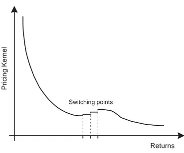
Returns

Pricing Kernel

Switching points

Figure 2: EPK with the switching points.

holds for any realization rT of RT. From this observation it becomes clear that the pricing kernel is nonincreasing separately on the intervals [0, x₁[,]x₁, x₂[, ...,]x_m∞[, but it might fail to be monotone just at the switching points x1, ..., xm (see figure 2).

For illustration let us assume that the distribution of R_T has [0,∞[ as support, and that the investors have an identical switching point say x0.That means

1_[0,x0](rT)du¹_α(rT,·) dy

y=rT + 1_]x0,∞[(rT)du^m+1_α (rT,·) dy

y=rT =zK_π(rT) for every realization rT of RT.

Furthermore, let us suppose that each investoriswitches between CRRA utilitiesu^j_i(y) =y^γji/γ^j_i (j= 0,1) with 0 < γ_i¹ < γ_i⁰ < 1, inducing the Arrow-Pratt coefficients of absolute risk aversion β_i^j(y) = ^1−γ

j i

y

(j = 0,1;y > 0). It follows β_i¹(y) > β₁⁰(y) for i ∈ {1, ..., m} and y > 0, which means that u¹₁, ..., u¹_m represent a more risk averse attitude than u⁰₁, ..., u⁰_m (cf. Mas-Colell et al. (1995), p. 191). In particular for stock prices lower or equal x₀ we have a bullish market, whereas we obtain a bearish market when stock prices exceedx0.

The application of Lemma B.1 and Proposition B.3 in Appendix B yields r_T =F⁰

du¹_α(rT,·) dy

_y=r

T

=F¹

du^m_α(rT,·) dy

_y=r

T

for any positive realization rT,where

F^j :]0,∞[→]0,∞[, z7→

m

X

i=1 αi>0

(z)

1 γj

i−1

αi

(j= 0,1)

are decreasing bijective mappings. Ifx₀>max{F⁰(1), F¹(1)},then du¹_α(r_T,·)

dy

y=rT,du^m_α(r_T,·) dy

y=rT <1, and

F⁰

du¹_α(rT,·) dy

y=rT

=rT =F¹

du^m_α(rT,·) dy

y=rT

> F⁰

du^m_α(rT,·) dy

y=rT

for any realizationr_T ≥x0.Therefore du^m+1_α (rT,·)

dy _y=r

T > du¹_α(rT,·) dy

_y=r

T forrT ≥x0. That means that Ke_π is not monotone atx0.

4 The Inverse Problems for the Switching Points

In section 3 we developed an economic environment, where in equilibrium the pricing kernelKe_π(R_T) may be expressed by a mixture of different marginal utilities. That means

Ke_π(RT) =

m

X

i=1

1_]xi−1,xi](RT)dui

dy _y=R

T+1_]xm,∞[(RT)dum+1

dy _y=R

T

for some m ∈ N, 0 = x₀ < ... < x_m < ∞ and mappings u₁, ..., u_m+1 : [0,∞] → R∪ {−∞} whose restrictions to ]0,∞[ are strictly increasing, strictly convex twice continuously differentiable real-valued functions satisfying the Inada conditions. Such a representation will be the starting point for the following investigations. The values x1, ..., xm will be called the switching points of the pricing kernel Ke_π(RT).

They are the amounts of returns where the investors are feeling themselves compelled to change their risk attitudes. Usually as a local measure of the risk aversion one might use the Arrow-Pratt coefficient of absolute risk aversion. Hence the change of the risk attitudes might be expressed by drawing a comparison of the left- and right-sided versions the Arrow-Pratt coefficients of absolute risk aversions at the switching

points. They read as follows

δ→0lim+

Ke_π(x_i−δ)−Ke_π(x_i) δ

Ke_π(x_i) , lim

δ→0+

Ke_π(x_i+δ)−Ke_π(x_i) δ

Ke_π(x_i) fori∈ {1, ..., m}.

Unfortunately, neither the number and the location of the switching points nor the marginal utilities of the u₁, ..., u_m+1are known. In order to get an idea of them we suggest to fit basic values of the pricing kernel.

For that purpose we fix a set V of strictly decreasing continuously differentiable mappings v :]0,∞[→ R satisfying lim

x→∞v(x) = 0.As a prominent example we mention the parameterized set of functionsv,defined by v(x) ^def= (x+a)^b−1 for some a ≥ 0 and b ∈]0,1[. These are the marginals of the generalized HARA (CRRA) utilities. As test functions for the data fitting we shall use mixtures

N

P

i=1

vi1_]xi−1,xi] of functions from V.Here the basic points represent approximately the unknown switching points. The quality of the approximation will be expressed by quadratic mean error w.r.t. a fixed continuous distribution ˆF with density function say ˆpand compact support enclosed in [0,∞[.The mapping ˆpmight be a kernel estimation of a density function for the distribution of RT. Henceforth we shall denote the minimum and maximum of the support byz and ¯z respectively.

We shall focus on the choice of appropriate basic points. The two approaches we want to propose differ in the way to discretize the pricing kernel.

4.1 The Monte Carlo Approach

For any distribution F on R satisfying F([z,∞[) = 1, we shall consider i.i.d. sequences (X_N^F)_N of random variables with common distribution F. Fixing N, they are associated with the order statistics X_1:N, ..., X_N:N according to z^def= X_0:N ≤X_1:N ≤...≤X_N:N.

The idea is to discretize randomly Ke_π by Ke^N_π(F) ^def=

N

P

i=1

Ke_π(X_i:N^F )1_]X^F

(i−1):N,X_i:N^F ].The suggestion is statis- tically motivated by the following observation.

Proposition 4.1 LetF be a continuous distribution onRwithF([z,∞[) = 1,and letC(Ke_π)denote the set of continuity points of Ke_π. Then for anyx∈ C(Ke_π) which belongs to the topological interiorint(supp(F)) of the support of F we obtain

N

X

i=1

Ke_π(X_i:N^F )1_]XF

(i−1):N,X_i:N^F ](x)→Ke_π(x) a.s..

In particular, setting i(F) ^def= inf{x |F(]− ∞, x])> 0} and s(F) ^def= sup{x |F(]− ∞, x]) <1}, we may even achieve this convergence for any x∈ C(Ke_π)∩]i(F), s(F)[ if supp(F) is konvex.

Proposition 4.1 is an immediate application of Proposition C.1 in appendix C.

The choice of proper basic points for the discretization changes into the problem to find a proper a priori distribution for the Monte Carlo sampling. The sample size N will be assumed to be given exogeneously.

Simulating the jumping behaviour of Ke_π in finite many points, we shall restrict ourselves to all continuous distributions with bounded support enclosed in [0,∞[, and which have density functions being constant on each interval ]xi−1, x_i[ (i= 1, ..., N) for some x₀ ≤ x₁ ≤ ... ≤ x_N, where x₀ and x_N denote a lower and an upper bound of the support respectively. In particular we consider the set P_N of all continuous distributions with bounded support enclosed in [z,z],¯ and which have density functions being constant on each interval ]xi−1, xi[ (i= 1, ..., N) for some z^def= x0 ≤x1 ≤...≤xN def

= ¯z.Furthermore for F ∈ P_N we shall denote the joint distribution of X_1:N^F , ..., X_N:N^F by F_(N).Then the inverse problem reads as follows.

Inverse problem:

Find F^∗ ∈ P_N such that

v1,...,vinfN∈V

Z EF_(N)^∗

"

Ke^N_π(F^∗)(x)−

N

X

i=1

v_i(x)1_]XF∗

(i−1):N,X_i:N^F∗](x)

#2

ˆ p(x) dx

= min

F∈PN(z) inf

v1,...,v_N∈V

Z EF_(N)

"

Ke^N_π (F)(x)−

N

X

i=1

v_i(x)1_]XF

(i−1):N,X_i:N^F ](x)

#2

ˆ p(x) dx

We shall discuss the solvability of the inverse problem after we shall have introduced the second inverse problem to be considered.

4.2 The pure numerical approach

The restrictionKe_π|[z,z] should be discretized by by some basic values. More precisely, we choose a partition¯ z ^def= x₀ ≤x₁ < ... < x_N ^def= ¯z of [z,z],¯ and use Ke^N_π(x₁, ..., x_N)^def=

N

P

i=1

Ke_π(x_i)1_]xi−1,xi] as an approximation of Ke_π|[z,z].¯ This idea suggests itself by the following observation.

Proposition 4.2 The mapping

N

P

i=1

Ke_π(a+_Nⁱ (b−a))1

]a+⁽ⁱ⁻¹⁾_N (b−a),a+_Nⁱ(b−a)] converges toKe_π|[a, b]uniformly on compacta of continuity points of K_π|[a, b]for any nondegenerated interval [a, b]⊆]0,∞[.

Proposition 4.2 may be derived immediately from the well known Korovkin like approximation result for mappings on [0,1] (cf. e.g. Witting and M¨uller-Funk (1995), Satz B5.2).

As for the Monte Carlo approach we shall not care about the choice of N, it will be assumed to be exogeneously given. Denoting byZ_N the set of all (x₁, ..., x_N)∈R^N satisfyingx₀ ^def= z≤x₁≤...≤x_N = ¯z, the choice of the basic points might be described in terms of the following inverse problem.

Inverse problem:

Find (x^∗₁, ..., x^∗_N)∈ Z_N such that

v1,...,vinfN∈V

Z ^N X

i=1

h

Ke_π(x^∗_i)−vi(x) i2

1_]x^∗

(i−1),x^∗_i](x) ˆp(x) dx

= inf

(x0,...,xN)∈Z_N inf

v1,...,vN∈V

Z ^N X

i=1

h

Ke_π(x_i)−v_i(x)i2

1_{]x(i−1),xi]}(x) ˆp(x) dx

As a convention we tacitly set Ke_π(0)^def= ∞ and ∞ ·0^def= 0.

4.3 Solvability of the inverse problems

Throughout this section we shall assume sup

v∈V

Z

v(x)^2+δp(x)ˆ dx <∞ for someδ >0.

Remark 4.3 In the following situations the familyV fulfills the assumed integrability condition:

1.

1

R

0

ˆ p(x)

x^2+δ dx <∞ for some δ >0, and V ^def=

v:]0,∞[→R, x7→(x+a)^b−1 |a≥0, b∈]0,1[ . 2. z >0,and sup

v∈V

v(z)<∞,e.g. if V ^def=

v:]0,∞[→R, x7→(x+a)^b−1|a≥0, b∈]0,1[ .

The integrability condition means thatV isL₂−norm bounded. In particularV as well as{v²|v∈ V}are uniformly ˆF−integrable, and the weak closure cl^w(V) of V is weakly compact because L2( ˆF), equipped with the L₂−norm, is a reflexive Banach space. Moreover, since the standard Borel σ−algebra on R is countably generated, the L2−norm topology on L2( ˆF) is separable. Hence the relative topology of the weak topology to cl^w(V) is metrizable (cf. Dunford and Schwarz (1958), Theorem V.6.3), and thus as a compact topology also separable. So we obtain the following result.

Lemma 4.4 Under the integrability condition on V the weak closure cl^w(V) of V is weakly compact, and the relative weak topology to cl^w(V) is separably metrizable.

For abbreviation let us define g:Z_N ×L2( ˆF)^N →R∪ {∞} by

g(x₁, ..., x_N, v₁, ..., v_N) =





 R P^N

i=1

(K(xi)−vi(x))²1_]xi−1,xi](x)ˆp(x) dx: (v1, ..., vN)∈ V^N

∞ : otherwise

Let us gather some basic properties of g.

Lemma 4.5 Letτ₁ be the relative topology of the standard topology onR^N toZ_N,letτ₂ denote the product weak topology on L2( ˆF)^N, and let τ1×τ2 stand for the product topology of τ1 and τ2. Furthermore let us denote the set of continuity points ofKe_π by C(Ke_π).Then under the integrability condition onV the mapping g satisfies the following properties:

1. g(x1, ..., xN,·)| V^N is lower continuous w.r.t. τ2 for every(x1, ..., xN)∈ Z_N;

2. g(·, v₁, ..., v_N) is measurable w.r.t. the Borel σ−algebra generated by τ₁ for any (v₁, ..., v_N) ∈ V^N, and the restrictions of these mappings to Z_N ∩ C(Ke_π)^N are even continuous w.r.t. τ1;

3. The family n

g(·, v)|Z_N ∩ C(Ke_π)^N

v∈ V^No

is equicontinuous w.r.t. τ1,in particular the restriction of g to

Z_N ∩ C(Ke_π)^N

× V^N is lower semicontinuous w.r.t. τ₁×τ₂. Proof:

The statement 1. may be verified by routine procedures. For that purpose it should be observed that we may restrict ourselves to sequential weak lower semicontinuity by Lemma 4.4 and that the squared L₂−norm is weakly lower semicontinuous as a convex L₂−norm continuous mapping.

Statement 2. follows easily from measurability of Ke_π and the following observation (*) For every ε1 >0,there is someε2 >0 such that

sup

w∈W

Z

|w(x)|

1_]y1,y2](x)−1_]z1,z2](x)

p(x)ˆ dx < ε1

whenever (y1, y2),(z1, z2) ∈[0,∞[² withy1 ≤y2, z1 ≤z2 and (y1−z1)²+ (y2−z2)² < ε2. Here W denotes an arbitrary familiy of uniformly ˆF−integrable real-valued mappings on ]0,∞[.

In order to see (*) observe R

1_]y1,y2]−1_]z1,z2]

p(x)ˆ dx =R

1_]y1,y2[−1_]z1,z2[

p(x)ˆ dx → 0 as (z1, z2) → (y₁, y₂),and that

1_]y1,y2]−1_]z1,z2]

is just indicator function of the symmetric difference of the involved intervals.

For the proof of statement 3. it suffices to show τ₁−equicontinuity of n

g(·, v)|Z_N ∩ C(Ke_π)^N

v∈ V^No because the second part of statement 3. follows then in view of statement 1.. So let us fix some (x1, ..., xn)∈ Z_N∩ C(Ke_π)^N.SinceZ_N∩ C(Ke_π)^N ∈τ₁,we may find a bounded neighbourhood U ∈τ₁ of (x₁, ..., x_n) such thatU ⊆ C(Ke_π)^N∩[ρ,z]¯^Nfor someρ >0.Then we obtain for any (˜x1, ...,x˜N)∈Uand any (v1, ..., vN)∈ V^N

|g(x₁, ..., x_N, v₁, ..., v_N)−g(˜x₁, ...,x˜_N, v₁, ..., v_N)|

≤

N

X

i=1

Z

Ke_π(x_i)−v_i(x)2

1_]xi−1,xi]−1_{]˜xi−1,˜xi]}

p(x)ˆ dx +

N

X

i=1

Z

Ke_π(xi)−vi(x) 2

−

Ke_π(˜xi)−vi(x) 2

1_{]˜xi−1,˜xi]} p(x)ˆ dx

≤

N

X

i=1

sup

v∈V

Z

Ke_π(x_i)−v(x)2

1_]xi−1,xi]−1_{]˜xi−1,˜xi]}

p(x)ˆ dx +

N

X

i=1

sup

v∈V

Z

Ke_π(xi)−v(x) 2

−

Ke_π(˜xi)−v(x) 2

1_{]˜xi−1,˜xi]} p(x)ˆ dx

≤

N

X

i=1

sup

v∈V

Z

Ke_π(x_i)−v(x)2

1_]xi−1,xi]−1_{]˜xi−1,˜xi]}

p(x)ˆ dx +

N

X

i=1

Ke_π(xi)−Ke_π(˜xi) sup

v∈V

Z

Ke_π(xi) +Ke_π(˜xi) + 2v(x)

ˆ p(x)dx

Since we have assumedKe_π to be a piecewise decreasing positive function,Ke_π|[ρ,z] is bounded from above¯ by some positiveδ.Additionally, sup

v∈V

Rv(x) ˆp(x)dx <∞by weak compactness ofcl^w(V),and

v² |v∈ V is uniformly ˆF−integrable due the integrability condition on V.Therefore, on one hand

N

X

i=1

Ke_π(x_i)−Ke_π(˜x_i) sup

v∈V

Z

Ke_π(x_i) +Ke_π(˜x_i) + 2v(x) ˆ p(x) dx

≤

2δ+ 2 sup

v∈V

Z

v(x) ˆp(x) dx N

X

i=1

Ke_π(xi)−Ke_π(˜xi) .

On the other hand

[K(x)−v]² |x∈[ρ,z], v¯ ∈ V is uniformly ˆF−integrable (cf. Bauer (1992), Korollar 21.3), and we may apply (*). Putting all together, the equicontinuity of n

g(·, v)|Z_N ∩ C(Ke_π)^N

v∈ V^No

at (x1, ..., xN) follows immediately, completing proof.

Next let us introduce the lower semicontinuous envelopelsc(g) ofg,defined to be the largestτ₁×τ₂−lower semicontinuous R∪ {∞}−valued mapping dominated by g. Notice that g and lsc(g) coincide on the set

Z_N ∩ C(Ke_π)^N

× V^N by Proposition 3.6 in DalMaso (1993).

The lower semicontinuous envelope will turn out to be a useful tool concerning the solvability of the inverse problems posed in the subsections before. Let us begin with the one coming out of the pure numerical approach. In terms of g it reads as follows.

minimize inf

v∈V^Ng(x₁, ..., x_N, v) among all (x1, ..., xN)∈ Z_N.

Fortunately, we may apply directly Theorem 3.8 in DalMaso (1993), observing that Z_N ×cl^w(V)^N is compact and sequentially compact w.r.t. τ1×τ2,and by Lemma 4.5

m→∞lim

inf

v∈V^Ng(x_m, v)− inf

v∈V^Ng(x₀, v)

≤ lim

m→∞ sup

v∈V^N

|g(x_m, v)−g(x₀, v)|= 0 for any sequence (x_m)m∈N0 inZ_N ∩ C(Ke_π)^N ∈τ₁ withx_m→x₀.

Theorem 4.6 Let (x_m, v_m)

m be a sequence in Z_N× V^N such that lim

m→∞g(x_m, v_m) = inf

x∈ZN

inf

v∈V^Ng(x, v).

Then this sequence has at least one cluster point in Z_N ×cl^w(V)^N, and every such cluster point (x^∗, v^∗) satisfies

lsc(g)(x^∗, v^∗) = min

(x,v)∈Z_N×cl^w(V)^Nlsc(g)((x, v) = inf

(x,v)∈Z_N×V^Ng(x, v), with inf

v∈V^Ng(x^∗) = inf

x∈Z_N inf

v∈V^Ng(x, v) if the components of x^∗ are continuity points of Ke_π.

In view of Tonelli’s theorem the inverse problem we have formulated after introducing the Monte-Carlo approach may be described in terms ofg by

minimize inf

v∈V^NEF_(N)

g(X_1:N^F , ..., X_N^F_:N, v) among allF ∈ P_N.

Theorem 4.7 Let τw be the topology of weak convergence on the set of distributions onR,and let τw×τ2

denote the product topology ofτ_w and the product weak topologyτ₂ onL₂( ˆF)^N.Furthermore let us consider a sequence ((Fm, v_m))_m in P_N × V^N fulfilling

m→∞lim EF_m(N)

h

g(X_1:N^Fm, ..., X_N^Fm_:N, v_m) i

= inf

F∈P_N inf

v∈V^NEF_(N)

g(X_1:N^F , ..., X_N^F_:N, v) .

Then this sequence has a cluster point w.r.t. to τw×τ2.Every such cluster point(F^∗, v^∗) satisfies min

n lim inf

m→∞ EF_m(N)

h

g(X_1:N^Fm, ..., X_N^Fm_:N,˜v_m) i

|˜v_m →v^∗ o

= min

v∈L2( ˆF)^N

minn lim inf

m→∞ EF_m(N)

h

g(X_1:N^Fm, ..., X_N:N^Fm ,v˜_m)i

|˜v_m →vo

= inf

F∈P_N inf

v∈V^NEF(N)

g(X_1:N^F , ..., X_N:N^F , v) ,

where even inf

v∈V^NEF^∗

g(X_1:N^F , ..., X_N:N^F , v)

= inf

F∈P_N inf

v∈V^NEF_(N)

g(X_1:N^F , ..., X_N:N^F , v)

holds if z > 0, and the set of discontinuity points of Ke_π is a F^∗−null set (e.g. ifF^∗ is a continuous distribution).

Proof:

First of all, since the topology of weak convergence for distributions onRis completely as well as separably metrizable, and since the supports of the distributions F_m are uniformly enclosed in a compact subset of R, the sequence (Fm)m is uniformly tight, and therefore has a cluster point by Prokhorov’s theorem.

Furthermore cl^w(V)^N has been observed as sequentially τ₂−compact by Lemma 4.4, so that we may conclude that ((Fm, v_m))_m has a cluster point w.r.t. τw×τ2.

Now, let (F^∗, v^∗) be a cluster point of ((F_m, v_m))_m. Without loss of generality we may assume that it is even a limit point. Then the induced sequence (F_m(N))m of the respective joint distributions of the order statisticsX_1:N^Fm, ..., X_N^Fm_:N has the joint distributionF_(N)^∗ of X_1:N^F∗, ..., X_N:N^F∗ as a limit point w.r.t. the topology of weak convergence on the set of distributions on R^N.Indeed, denoting the joint distribution of the order statistics U_1:N, ..., U_N:N obtained from an i.i.d sample of size N according to the uniform distribution on ]0,1[ by F_U,(N), we have F_m(N)

i=1

N ]− ∞, x_i]

= F_U,(N)

i=1

N ]− ∞, F_m(]− ∞, x_i])]

for any (x1, ..., x_N)∈R^N,and an analogous expression for F_N^∗. Then the claim follows immediately from the Helly Bray theorem.