www.biogeosciences.net/14/1647/2017/
doi:10.5194/bg-14-1647-2017
© Author(s) 2017. CC Attribution 3.0 License.
Reviews and syntheses: parameter identification in marine planktonic ecosystem modelling
Markus Schartau1, Philip Wallhead2, John Hemmings3,a, Ulrike Löptien1, Iris Kriest1, Shubham Krishna1, Ben A. Ward4, Thomas Slawig5, and Andreas Oschlies1
1GEOMAR Helmholtz Centre for Ocean Research Kiel, Kiel, Germany
2NIVA, Norwegian Institute for Water Research, Bergen, Norway
3Wessex Environmental Associates, Salisbury, UK
4University of Bristol, School of Geographical Sciences, Bristol, UK
5Christian-Albrechts-Universität zu Kiel, Department of Computer Science, Kiel, Germany
anow at: Met Office, Exeter, UK
Correspondence to:Markus Schartau (mschartau@geomar.de) and Phil Wallhead (philip.wallhead@niva.no) Received: 3 June 2016 – Discussion started: 20 June 2016
Revised: 17 February 2017 – Accepted: 21 February 2017 – Published: 29 March 2017
Abstract. To describe the underlying processes involved in oceanic plankton dynamics is crucial for the determination of energy and mass flux through an ecosystem and for the estimation of biogeochemical element cycling. Many plank- tonic ecosystem models were developed to resolve major processes so that flux estimates can be derived from numeri- cal simulations. These results depend on the type and number of parameterizations incorporated as model equations. Fur- thermore, the values assigned to respective parameters spec- ify a model’s solution. Representative model results are those that can explain data; therefore, data assimilation methods are utilized to yield optimal estimates of parameter values while fitting model results to match data. Central difficul- ties are (1) planktonic ecosystem models are imperfect and (2) data are often too sparse to constrain all model param- eters. In this review we explore how problems in parameter identification are approached in marine planktonic ecosys- tem modelling.
We provide background information about model uncer- tainties and estimation methods, and how these are consid- ered for assessing misfits between observations and model results. We explain differences in evaluating uncertainties in parameter estimation, thereby also discussing issues of pa- rameter identifiability. Aspects of model complexity are ad- dressed and we describe how results from cross-validation studies provide much insight in this respect. Moreover, approaches are discussed that consider time- and space-
dependent parameter values. We further discuss the use of dynamical/statistical emulator approaches, and we elucidate issues of parameter identification in global biogeochemical models. Our review discloses many facets of parameter iden- tification, as we found many commonalities between the ob- jectives of different approaches, but scientific insight differed between studies. To learn more from results of planktonic ecosystem models we recommend finding a good balance in the level of sophistication between mechanistic modelling and statistical data assimilation treatment for parameter esti- mation.
1 Introduction
The growth, decay, and interaction of planktonic organisms drive the transformation and cycling of chemical elements in the ocean. Understanding the interconnected and com- plex nature of these processes is critical to understanding the ecological and biogeochemical function of the system as a whole. The development of biogeochemical models re- quires accurate mathematical descriptions of key physiologi- cal and ecological processes, and their sensitivity to changes in the chemical and physical environment. Such mathemati- cal descriptions form the basis of integrated dynamical mod- els, typically composed of a set of differential equations that allow credible computations of the flux and transformation
of energy (light) and mass (nutrients) within the ecosystem (US Joint Global Ocean Flux Study Planning Report Num- ber 14,Modeling and Data Assimilation, 1992).
Generalized mechanistic descriptions of how energy is absorbed and how mass becomes distributed in an ecosys- tem already exist, such as dynamic energy budget models (Kooijman, 1986) or the metabolic theory of ecology (Brown et al., 2004). But these theories still have limitations, and in- clude incompatible assumptions (van der Meer, 2006). So far no fundamental ecophysiological principle has been further consolidated beyond the conservation of mass. A consistent theme running through most ecosystem models is the deter- mination of mass flux of certain biologically important ele- ments, such as nitrogen, phosphorus, iron, and carbon (N, P, Fe, and C). Nonetheless, the precise details of how mass is transformed and allocated within an ecosystem is far from being established. For this reason, we find a large variety of plankton ecosystem models that differ in their number of state variables as well as in their parameterization of individ- ual physiological and ecological processes.
1.1 Mass flux induced by plankton dynamics
Dynamical marine, as well as limnic, ecosystem models usu- ally start from a description of the build-up of biomass by photoautotrophic organisms (phytoplankton) as these take up dissolved nutrients from the water column and exploit light energy by photosynthesis. Phytoplankton biomass, as a prod- uct of primary production, is subsequently removed by nat- ural mortality (cell lysis due to starvation, senescence, and viral attack), predation by zooplankton, and vertical export away from surface ocean layers via sinking of single or ag- gregated cells and of fecal pellets. Parameterizations of these three loss processes can be interlinked, e.g. grazing of phy- toplankton aggregates by large copepods. Depending on the trophic levels considered in a model, the predation among different zooplankton types (e.g. between herbivores, carni- vores, or omnivores) can be explicitly parameterized. Mor- tality and aggregation of phytoplankton cells and the excre- tion of organic matter (fecal pellets) by zooplankton act as primary sources of dead particulate organic matter (detritus) that can be exported to depth via sinking. Exudation by phy- toplankton and bacteria can be a major source of labile dis- solved organic matter that represents diverse substrates for remineralization. The transformation of particulate and dis- solved organic matter back to inorganic nutrients is param- eterized as hydrolysis and remineralization processes. Often hydrolysis and remineralization are assumed to be propor- tional to the biomass of heterotrophic bacteria, which is con- sidered in many models. Heterotrophic bacteria remain unre- solved in some models where microbial remineralization is parameterized only as a function of concentration and qual- ity of organic substrates.
At some level most models include a parameterization to account for the net effect of higher trophic levels that are not
explicitly resolved. This is usually formulated as a closure flux back to nutrient pools and whose rates simply depend on the biomass of the highest trophic level resolved. These clo- sure assumptions ensure mass conservation while neglecting the actual mass loss to higher trophic levels like fish, which would be subject to fish movements and changes in biomass on multi-annual scales rather than seasonal timescales. Every marine planktonic ecosystem model can thus be described as a simplification of the dynamics inherent to a system of nutri- ents, phytoplankton, zooplankton, detritus, dissolved organic matter, and possibly bacteria.
In many cases marine ecosystem models are embedded in an existing physical ocean model set-up that simulates envi- ronmental conditions, advection, and mixing of the biologi- cal and chemical state variables. Feedbacks from the ecosys- tem model states on physical variables can be relevant (e.g.
Murtugudde et al., 2002; Oschlies, 2004; Löptien et al., 2009;
Löptien and Meier, 2011), but are rarely considered in cur- rent marine biogeochemical studies.
1.2 Parameters of plankton ecosystem models
One of the most influential model approaches to studying the nitrogen flux through such a marine plankton ecosystem at a local site was proposed by Fasham et al. (1990). Their model involves 27 parameters and they stressed the invidi- ous situation of finding a reliable ecosystem model solution by choosing parameter values that are uncertain or unknown.
Laboratory measurements, as well as ship-based experiments with field samples, can provide information about the range of typical values for some parameters, for example the max- imum growth rate of photoautotrophs or the maximum in- gestion rate of herbivorous plankton. Other model parame- ters are extremely difficult to measure, like exudation rates of dissolved organic carbon by phytoplankton or by bacte- ria. Another difficulty is that parameter values from labora- tory experiments are often specific with respect to plankton species, temperature, and light conditions. Their values may not be directly applicable for ocean simulations where pa- rameter values need to be representative of a mixture of dif- ferent plankton species in a continuously varying physical environment. For example, for a natural composition of di- verse phytoplankton cells that all differ in their genotypic and phenotypic characteristics, we may expect values of some model parameters to follow a distribution rather than having a single fixed value.
In practice, there are always some fixed model parameters that need to be assigned values, whether they describe the behaviour of fixed plankton functional types or the distribu- tions of traits in a stochastic community. In the end, it is the choice of these parameter values that determines a specific model solution of any ecological or biogeochemical model set-up.
1.3 The vital role of observational data
Model solutions of interest are typically those that can simu- late and explain complex data. Model calibration, which can be considered a form of data assimilation (DA), is the pro- cess by which model parameter values are inferred from the observational data. Optimal parameter values are regarded as those that generate model results that match observations (minimize the data–model misfit) but that are also in accor- dance with the range of values known e.g. from experiments or from preceding DA studies. To determine optimal parame- ter estimates we have to account for uncertainties in data and in model dynamics as well, which is specified by an error model. Parameter estimates are thus conditioned by (a) the dynamical model equations, (b) the data, (c) our prior knowl- edge about the range of possible parameter values, and (d) the underlying error model (Evans, 2003).
Situations can occur where model results that are com- pared with data are insensitive to variations of some param- eters. Values of those parameters remain unconstrained by the available data, which is a problem of parameter iden- tifiability. The availability (type and number) of data thus places limitations on the number of model parameters whose values become identifiable, and values of some parameters may never be fully constrained. This in turn sets restrictions on the complexity of plankton interactions that can be un- ambiguously confined during ecosystem model calibration (Matear, 1995). Choosing appropriate model complexity is ambiguous and is still subject to discussion (e.g. Franks, 2002, 2009; Denman, 2003; Fulton et al., 2003; Anderson, 2005; Le Queré, 2006; Friedrichs et al., 2007; Kriest et al., 2012; Ward et al., 2013), a situation which sustains large dif- ferences in the level of complexity of current plankton mod- els.
1.4 Inferences from data assimilation
Much of the literature on DA in oceanography is focussed on state estimation (e.g. Allen et al., 2003; Natvik and Evensen, 2003; Dowd, 2007; Nerger and Gregg, 2008; van Leeuwen, 2010). In these studies, the primary objective is to improve hindcasts, nowcasts, or forecasts of time-dependent variables such as chlorophyll a (Chl a). However, many of the DA methods originally developed for state estimation have more recently been adapted to estimate static parameters, espe- cially for stochastic models where random noise is injected into the model dynamics. Stochastic noise offers a plausible way to represent model error, but it should be noted that it can lead to violations of mass conservation unless it is in- jected in certain ways (e.g. by perturbing growth rate param- eters). Deterministic plankton ecosystem models guarantee mass conservation and have a longer tradition in parameter estimation for marine ecosystem models, although they im- ply a less explicit treatment of model error. To identify and gradually eliminate model deficiencies it can be helpful to
analyse model state and flux estimates while mass conser- vation is imposed as a strong constraint. The optimization of parameter values only ensures that simulation results re- main dynamically and ecologically consistent, which is com- parable with those DA approaches in physical oceanography that produce dynamically and kinematically consistent solu- tions of ocean circulation (e.g. Wunsch and Heimbach, 2007;
Wunsch et al., 2009).
Thorough reviews of common DA methods applied in ma- rine biogeochemical modelling are given by Robinson and Lermusiaux (2002) and by Matear and Jones (2011). Dowd et al. (2014) provide a helpful and up-to-date overview of mainly sequential DA approaches where state estimation is combined with parameter estimation. Gregg et al. (2009) and Stow et al. (2009) discuss how the success of DA re- sults of marine ecosystem models has been evaluated in the past and how model performance can be generally assessed.
Fundamentals on DA that include aspects relevant to marine ecosystem and biogeochemical modelling are explained in Wikle and Berliner (2007) and in Rayner et al. (2016).
In our review we primarily focus on topics related to parameter identification, thereby including basic aspects of DA. Parameter identification in marine planktonic ecosys- tem modelling is a wide field and we do not attempt to dis- cuss differences between various DA tools or techniques. We rather put emphasis on models, including parameterizations of ecosystem processes, statistical (error) models, model un- certainties, and structural complexity. We adopt and explain mathematical notation that is often used for DA studies in operational meteorology and oceanography. On the one hand we provide background information that should facilitate in- telligibility when studying DA literature. On the other hand we like to elucidate typical objectives and common problems when simulating a marine planktonic system. In this manner we hope to support a mutual understanding between ecologi- cally/biogeochemically and mathematically/statistically mo- tivated studies.
The paper starts with some theoretical background in- formation (Sect. 2), introducing mathematical notation and depicting prevalent assumptions that are typically made for parameter identification analyses and model calibration (Sect. 2.1). We then branch off from DA theory and discuss the parameters typically dealt with in plankton ecosystem models. In Sect. 3 we disentangle major differences between approaches to parameterizing photoautotrophic growth and briefly discuss simple but common parameterizations of plankton loss rates. In this context we also address the uti- lization of data from laboratory and mesocosm experiments.
Error models are described in order to elucidate error as- sumptions made in previous ecosystem modelling studies (Sect. 4). This is followed by a description of different approaches to specifying uncertainties in parameter values (Sect. 5). An example of parameter estimation with simula- tions of a mesocosm experiment connects aspects of Sect. 3 with the theoretical considerations of Sect. 5. Thereafter,
model complexity is jointly addressed together with cross- validation in Sect. 6, followed by a review of space–time variations in marine ecosystem model parameters (Sect. 7).
Emulator, or surrogate-based, approaches are briefly ex- plained and exemplified (Sect. 8) before we discuss pa- rameter estimation of large-scale and global biogeochemical ocean circulation models (Sect. 9). Finally, we summarize the insights that we gained into parameter identification in Sect. 10, and we will briefly address prospects of some ma- rine ecosystem model approaches that could improve param- eter identification.
2 Theoretical background
The term parameter identification is used broadly to describe parameter estimation problems, including the specification of uncertainties in parameter estimates and model parame- terizations. It involves the following procedures.
a. Parameter sensitivity analyses: the evaluation of how model results change with variations of parameter val- ues.
b. Parameter estimation: the calibration of model results by adjusting parameter values in light of the data.
c. Parameter identifiability analyses: the specification of parameter uncertainties in order to reveal structural model deficiencies and shortages in data availabil- ity/information.
All three aspects are interrelated and should not be viewed as mutually exclusive procedures. For example, before starting with parameter estimation it is helpful to include information from a preceding sensitivity analysis, e.g. selecting only pa- rameters to which model results are sensitive. Likewise, an identifiability analysis complements the sensitivity analysis by providing information about error margins and possible ambiguities of optimal parameter estimates.
2.1 Statistical model formulation
2.1.1 Model states, parameters, and dynamical model errors
The prognostic dynamical equations of a marine ecosystem model can be expressed as a set of difference equations:
xi+1=M
xi,θe,fi,ηi θη
, (1)
with indexirepresenting a particular time step (i.e.ti). The model state vector xi has dimension Nx=Ng×Ns where Ngis the number of spatial grid points andNsis the number of model state variables (e.g. phytoplankton biomass). The dynamical model operatorMis typically at least a nonlinear
function of the earlier statexi, a set of ecosystem parame- tersθe describing rate constants and coefficients in the dy- namical model, and a set of time- and space-dependent forc- ings and boundary conditions fi. If the ecosystem model is coupled “online” with a physical ocean model, fi in- cludes both physical model forcings (e.g. wind stress) and ecosystem model forcings (e.g. surface short-wave irradi- ance). If the physics is coupled “offline”,fiincludes ecosys- tem model forcings and physical model outputs (e.g. seawa- ter temperature).
For stochastic dynamical models,Malso depends on ran- dom noise variables or dynamical model errors ηi, while for deterministic models we haveηi=0. These errors are described by distributional parametersθη, e.g. location and scale parameters of a probability density function. Dynami- cal model errors usually enter the dynamics additively, mul- tiplicatively, or as time- or space-dependent corrections tof or θe. They may represent the individual or combined ef- fects of errors in forcings, boundary conditions, random vari- ability in model parameters, and structural errors in both the physical transport model (e.g. due to limited spatial resolu- tion) and the biological source-minus-sink terms (e.g. due to aggregation of species into model groups). In the geo- physical DA community, error models that explicitly account for dynamical model errors (noise) are often termedweak constraint models, while those that assume a deterministic model are termedstrong constraint(Sasaki, 1970; Bennett, 2002, p. 25).
2.1.2 True states and kinematic model errors
To relate the dynamical model output of Eq. (1) to obser- vations, it is helpful to first consider how it may relate to a conceptual and hypothetical true statext, which is then im- perfectly observed. In this respect we must also consider the averaging scales. In marine ecosystem modelling there is al- most always a large discrepancy between the spatio-temporal averaging scales of the model, which define the meaning of the “concentrations” in x, and the averaging scales of the observations from in situ sampling or remote sensing. For example, the spatial averaging scale of a model may be de- fined by a model grid cell of size 10 km in the horizontal and 10 m in the vertical, while the averaging scale of the observa- tions might be the 10 cm scale, e.g. of a Niskin bottle sample.
Even with a perfect model, data from fine-scale observations may diverge from model output due to unresolved sub-grid- scale variability induced by fluid structures such as eddies and fronts, forming patches of high next to low concentra- tions e.g. of nutrients or organic matter.
A general relationship between the true state and model state can be expressed as
xt=T
x,ζ θζ
, (2)
whereT is a truth operator, andζis a set of random variables described by distributional parametersθζ. We will refer to
theζ askinematicmodel errors because they are associated with the model state, while thedynamicalmodel errorsηin Eq. (1) act to perturb the model dynamics. The true values of the kinematic model errors therefore define the potential discrepancy between the target true state and a hypothetical ideal model output (i.e. with the “true” values of the param- eters and, if applicable, also with the “true” values of the dynamical model errors).
How we interpret and specify Eq. (2) depends on the spatio-temporal averaging scales chosen to define the true state xt, which in turn depends on the objectives of the modelling study. One approach is to define these averaging scales as equal to or larger than the shortest space scales and timescales that are fully resolved by the model. Kinematic model errors ζ may then represent the integrated effects of the various dynamical sources of model error, if these are not already accounted for by dynamical model errorsηin Eq. (1).
Alternatively, the true state can be defined over scales smaller than those resolved by the model, possibly at the scales of the observations. This may lead to a simpler model for ob- servational error (see below), but now theζmust account for the unresolved scales, in addition to any error effects in the model dynamics otherwise not accounted for. With stochas- tic dynamical models (η6=0), the true state is usually defined on the scales of the model and assumed to coincide with the model output for some (θe,η), such that no kinematic error model is needed.
2.1.3 Data and observational errors
The observation vectorycan be related to the true state via y=O
xt,(θ)
, (3)
where O is the generalized observation operator and is a set of randomobservationalerrors described by distribu- tional parametersθ and accounting for uncertainties asso- ciated with the usage and interpretation of the data. These include at least the random measurement error due to, for example, instrument noise. In addition they may include a contribution fromrepresentativenesserror due to fine-scale variability, if xt is defined as an average over larger scales than those of the observations (see above). Alternatively, if the observations are preprocessed into estimates on the larger scales ofxt, there may be anundersamplingerror component due to inexhaustive coverage of the raw samples. The obser- vation operatorOmay also contribute to, for example if the model output needs to be interpolated from the model grid to the data coordinates, or ifOincludes conversion factors such as chlorophylla-to-nitrogen (Chla: N) ratios.
The simplest possible example of an observational error model assumes additive Gaussian errors. Equation (3) then becomes
y=H xt +
−→=y−H xt
, (4)
whereHaccounts for interpolation and units conversion and ∼G(0,R)is Gaussian distributed with mean zero and co- variance matrix R. This may be a reasonable error model for most physical variables and chemical concentrations with ranges well above zero (e.g. dissolved inorganic carbon or total alkalinity in the open ocean). However, many nutrients and plankton biomass variables may vary close to their lower bounds of zero, and display positive skew in their observa- tional errors. For such variables, a lognormal observational error model may be more appropriate:
y=H xt
◦exp e−eσ2 2
!
−→e=log(y)−log H xt +eσ2
2 , (5)
where ◦ denotes element-wise multiplication and eσ2 de- notes the variance in logarithmic space. The bias-correction term (eσ2/2) ensures unbiased errors, but is frequently ne- glected in practice. The various options and challenges of defining an appropriate error model are discussed in detail in Sect. (4).
2.2 Estimation methods
2.2.1 Basic probabilistic approaches
We now consider how to estimate uncertain parameters2 given the datay, where2 includes all biological parame- tersθe and possibly distributional parameters (θη, θζ,θ).
There are basically two probabilistic approaches for doing this: Bayesian estimation and maximum likelihood estima- tion. In the Bayesian approach, we treat the parameters as random variables, and choose parameter values on the basis of their “posterior probability”, i.e. the conditional probabil- ity density of the parameter values given the datap(2|y).
The posterior probability is computed using Bayes’ theorem:
p(2|y)=p(y|2)·p(2)
p(y) ∝p(y|2)·p(2), (6) wherep(y|2)is the likelihood andp(2)is the uncondi- tional or “prior” distribution of the parameter values. The proportionality follows in Eq. (6) because the probability of the data p(y), otherwise known as the “evidence” for the model, is independent of the parameter values.
In general the likelihood can be expressed as an integral over probabilities conditioned on particular values of the model state and true state:
p(y|2)= Z Z
p(y|xt,2)·p(xt|x,2)·p(x|2)dxtdx, (7) where the conditional probabilitiesp(y|xt,2),p(xt|x,2), andp(x|2)are specified by the chosen models for observa- tional error (Eq. 3), kinematic model error (Eq. 2), and dy- namical model error (Eq. 1) respectively. In practice we are unlikely to require such a complex expression for numerical evaluation; aggregation of error terms and redundancy be- tween kinematic and dynamical model error usually allows simplifications.
The Bayesian approach encourages us to explicitly quan- tify our prior knowledge about the parameter values through the priorp(2). In marine ecosystem modelling, we are un- likely to ever consider cases of complete parameter igno- rance, where a parameter value could possibly switch sign or get incredibly large. Every parameter is expected to have a value that falls into a credible range; otherwise, the associ- ated parameterization would be difficult to defend. In some cases, when broad uniform or “uninformative” priors are as- sumed, it may not be necessary to specify exact limits of these distributions as the analyses may become insensitive to these limits once the range becomes sufficiently broad. There are inherent difficulties with the concept of “ignorance” pri- ors: for example, a flat prior distribution over φwill corre- spond to an informative prior for some function g(φ) (see Cox and Hinkley, 1974, for further discussion). In any case, trying to minimize the impact of prior distributions rather de- feats the object of Bayesian estimation, which explicitly aims to synthesize information from new data with prior informa- tion from previous analyses.
Once the likelihood is formulated and a prior distribution is prescribed, classical Bayes estimates (BEs) may be com- puted from posterior mean or posterior median values of2.
Assuming the statistical assumptions are correct, these esti- mators will minimize the mean square error or mean absolute error respectively of the parameter estimate 2b (e.g. Young and Smith, 2005). To obtain BEs can be computationally expensive, requiring sophisticated techniques to sample effi- ciently from the posterior distribution (e.g. by Markov chain Monte Carlo, MCMC, methods). An alternative Bayesian es- timator, very widely used in geosciences, is the joint poste- rior mode or maximum a posteriori (MAP) estimator (e.g.
Kasibhatla, 2000; Bocquet, 2014), given by maximizing the posterior probabilityp(2|y)as a function of2. Such esti- mates are more computationally feasible in large problems where the search for the maximum of the posterior (or the minimization of its negative logarithm) can be greatly accel- erated by techniques such as the variational adjoint (Bennett, 2002, Chap. 4).
In maximum likelihood (ML) estimation we seek the pa- rameter values2bMLthat maximize the probability of the data given the parameter set, i.e.p(y|2). When considered as a function of2, this probability is called thelikelihoodof the parameter valuesL(2|y)because it is strictly a probability of the data, not of the parameter values. Indeed, in ML esti- mation we do not need to consider the parameter values as random variables at all; rather they are considered as fixed, unknown constants. For this reason the “|”s are sometimes replaced by “;”s to emphasize that, in a non-Bayesian con- text, the likelihood is not a conditional probability in the sense of one set of random variables dependent on another (e.g. Cox and Hinkley, 1974). In the ML approach, no prior information on the parameter values is used except possibly to define upper or lower plausible limits or allowed ranges for the parameter search (Young and Smith, 2005).
Historically, Bayesian methods (Bayes, 1763; Bayes and Price, 1763) predate ML methods of Fisher (1922) by some margin. Fisher introduced ML methods partly to avoid prob- lems in defining prior ignorance (see above) but also to avoid the noninvariance property of Bayesian estimators (Hald, 1999). This property means that given the BE of one param- eterbφB, the corresponding BE of a nonlinear function of that parameterg(φ)is not simply given by plugging in the es- timate (bgB6=g(bφB)), while for ML estimates the invariance property does hold (bgML=g(bφML)). We will see an example of this in Sect. 2.3.
2.2.2 Sequential methods
In some problems, assimilating all the data at once from all available sampling times can be computationally impractical.
This is particularly likely for models with stochastic dynam- ics (η6=0 in Eq. 1), if the data are clustered in time, or if model states need to be repeatedly updated as new data come in. In such cases a sequential approach can be expedient. The basic idea is to break the large integration problem defined by Eq. (7) into a number of smaller problems by sequentially as- similating observations in subsets defined by sampling time.
The method comprises a consecutive sequence of two ma- jor steps: a forecast step and an analysis step. If the sequen- tial algorithm is accurate, it should approximate the posterior parameter distribution defined by Eqs. (6) and (7) at times where all available data have been assimilated.
To see how this works, suppose we know the probability densityp(xtj|y1:j,2)of the true state at sampling timetj (possibly an initial condition) for a given value of the uncer- tain parameters2 and given all the previously assimilated observationsy1:j (possibly null). The probability density at sampling timetj+1is given by the forecast density:
p
xtj+1|y1:j,2
= Z
p
xtj+1|xtj,2
·p
xtj|y1:j,2
dxtj. (8)
In general this integral can be approximated by an ensem- ble of Monte Carlo simulations, sampling an initial condition fromp(xtj|y1:j,2)and then running the model to the next sampling timetj+1(possibly including stochastic dynamical noise, and possibly accounting for kinematic model error).
Next, in the analysis step, the new observations are assimi- lated by applying Bayes’ theorem:
p
xtj+1|y1:(j+1),2
∝p
yj+1|xtj+1,2
·p
xtj+1|y1:j,2
, (9)
which again can be approximated e.g. by Monte Carlo sam- pling. The forecast and analysis steps can then be repeated until all the data are assimilated. Note that Eq. (9) assumes conditional independence of the observations, allowing us to write p(yj+1|xtj+1, 2) instead of p(yj+1|xtj+1, y1:j, 2). This amounts to assuming that the observational errors are independent between sampling times (Evensen, 2009), which may not be strictly true if sampling is frequent and if there is a noticeable contribution from representative- ness/undersampling, or from errors in conversion factors (see Sect. 2.1.3).
Once the predictive filtering densities p(xtj+1|y1:j, 2) have been approximated for all sampling times (tj with j=1, . . . , Nt), these can be used to approximate the like- lihood in Eq. (7), since
p(y|2)=
Nt
Y
j=1
p yj|y1:j−1,2
=
Nt
Y
j=1
Z p
yj|xtj,y1:j−1,2
·p
xtj|y1:j−1,2 dxtj
=
Nt
Y
j=1
Z p
yj|xtj,2
·p
xtj|y1:(j−1),2
dxtj. (10) For j=1 in Eq. (10) we have a set of zero members and p(yj|y1:j−1,2)=p(y1|2). The third line of Eq. (10) again assumes conditional independence of the observations and the final integral can in general be approximated using the predictive ensembles (see Jones et al., 2010; Dowd, 2011;
Dowd et al., 2014). This procedure can be repeated for differ- ent values of2and combined with Eq. (6) to assess posterior probability.
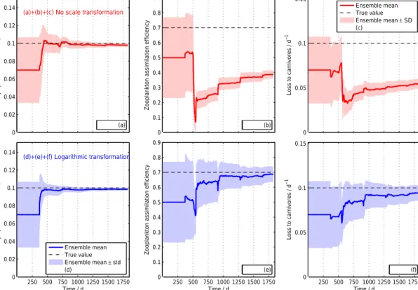
Alternatively,p(2|y)can be calculated from a single ap- plication of the filter using a “state augmentation” approach whereby the parameters2 are appended to the vectorxas additional state variables with zero dynamics. In practice, random parameter noise may need to be added to avoid filter degeneracy, such that this approach may be considered a sep- arate estimation method (Dowd, 2011). However, if such ad hoc noise can be avoided, or if the parameters are in fact as- sumed to vary stochastically, then the augmented-state filter at the end of the assimilation interval should approximate the
theoretical Bayesian posterior for this time. For other times, a “smoother” algorithm would be required. A further benefit of the augmented-state filter is that the parameter estimates for intermediate time periods may show temporal patterns that expose deficiencies in the model formulation and pro- vide useful information for model development (e.g. Losa et al., 2003).
The various types of filter differ essentially in terms of how the integrals in Eqs. (8) and (9) are approximated. Particle filters (van Leeuwen, 2009) use Monte Carlo sampling for both steps, while the ensemble Kalman filter (Evensen, 2003, 2009) uses Gaussian and linear approximations for the analy- sis step, enabling the use of smaller ensembles but at the cost of lower accuracy in strongly nonlinear/non-Gaussian prob- lems. The (extended) Kalman filter applies when the model dynamics are (quasi-) linear and both model and observa- tional errors are Gaussian. These conditions allow both inte- grals to be evaluated analytically, but appear to be rarely ap- plicable to parameter estimation in marine ecosystem mod- els. For reviews of sequential approaches the reader is re- ferred to Dowd et al. (2014) for marine biogeochemical mod- elling and to Bertino et al. (2003) for oceanography in gen- eral.
2.2.3 Variational methods
At present there appears to be some ambiguity regarding the term “variational” in the context of DA. It is sometimes used to describe approaches explicitly based on control theory or
“inverse methods” that may not include explicit assumptions about error distributions and where cost functions are de- fined a priori, rather than being derived from statistical or probabilistic models. However, a distribution-free approach seems difficult to recommend in general for marine ecosys- tem model parameter estimation, given the strong nonlinear- ity, non-Gaussianity, and relatively weak data constraint of- ten encountered in such problems. Within the marine ecosys- tem modelling community, the term “variational DA” is often used more broadly to refer to all non-sequential methods that involve the minimization of a cost function, whether or not this is based on a probability model.
In any case, there are some powerful mathematical tools developed for variational DA that can be applied to min- imize cost functions. Adjoint methods allow the gradient of the cost function with respect to all fitted parameters to be computed in an extremely efficient manner; see Lawson et al. (1995), and Appendix C. This is particularly useful when dealing with a large number of fitted parameters (high- dimensional2) of computationally expensive models (e.g.
Tjiputra et al., 2007). The application of the adjoint method helps to reduce the number of model runs to provide access to joint posterior mode and maximum likelihood estimates.
Pelc et al. (2012) provide useful theoretical background for different 4DVar approaches (four-dimensional, in space and time, variational approaches) and show how this adjoint
method can be used to estimate ecosystem model parameters jointly with a large number of initial condition parameters.
See also Bennett (2002) for an introduction to variational DA and adjoint methods in physical oceanography. However, it can be disadvantageous to employ a search algorithm that re- lies too much on local gradients (e.g. from an adjoint model) to minimize the cost function, because this may result in find- ing a local minimum rather than the global minimum that defines the MAP or ML estimate (Vallino, 2000). This issue appears to be frequently encountered in marine ecosystem modelling applications, and should be expected as a prod- uct of strong nonlinearity and weak data/prior constraint. For such cases, a non-local approach such as simulated anneal- ing, following Hurtt and Armstrong (1996, 1999), or a micro- genetic algorithm, following Schartau and Oschlies (2003), may be preferable, at least during an initial period of the search before the broader region of the global minimum is located (Ward et al., 2010). The main drawback of these non- local search algorithms is that they tend to require a larger number of model runs (of at least order 103) to have a good chance of accurately locating the global minimum, although they may yet provide meaningful improvements to prior pa- rameter estimates for an order of 100 runs (Mattern and Ed- wards, 2017).
2.2.4 Recent approaches
Much recent interest has focused on combined state and pa- rameter estimation, whereby model parameters 2are esti- mated together with a true statext(e.g. Simon and Bertino, 2012; Fiechter et al., 2013; Parslow et al., 2013; Weir et al., 2013; Dowd et al., 2014). In the Bayesian approach, model parameters and system state are both random variables.
We can therefore apply Bayes’ theorem to the composite random variable 9=(2, xt) and decompose the prior as p(9)=p(xt|2)·p(2)to obtain an expression for the joint posterior:
p xt,2|y
∝p y|xt,2
·p xt|2
·p(2). (11)
This equation has so far been applied to stochastic dynamic models with no kinematic model error (cf. Fiechter et al., 2013; Parslow et al., 2013). Equation (6) can be recov- ered from Eq. (11) by integrating (marginalizing) both sides overxt.
In some other recent studies emphasis is put on “hi- erarchical” error models (Zhang and Arhonditsis, 2009;
Parslow et al., 2013; Wikle et al., 2013). Here, the traditional model parameters are replaced with stochastic processes over time and/or space, and parameter identification focuses on the hyperparametersthat describe the stochastic processes (e.g. means, variances, autocorrelation parameters). This is essentially similar to the case of parameter estimation for a stochastic dynamical model (Sect. 2.2.2) and fits into the gen- eral formulation in Sect. 2.1, if we treat the stochastic param- eters as additional state variables with dynamical model er-
rorsη. The hyperparameters could in principle be estimated by ML, sometimes referred to as an “empirical Bayesian” ap- proach (Cox and Hinkley, 1974), but it appears that compu- tational tractability may favour the “hierarchical Bayesian”
approaches (e.g. Zhang and Arhonditsis, 2009), which may also make use of sequential Monte Carlo methods (e.g. Jones et al., 2010; Parslow et al., 2013).
Another important initiative is the estimation of hyperpa- rameters of the kinematic error model along with the ecosys- tem parameters (Arhonditsis et al., 2008). The posterior of the kinematic model error provides an estimate of the model discrepancy, introduced by Kennedy and O’Hagan (2001) and originally referred to as model inadequacy. The model discrepancy is defined as the model error for the “true” val- ues of the model parameters, i.e. the unknown values of the parameters for which the model best representsxt. Estimates of model discrepancies may thus provide useful diagnostics for model skill assessment and development.
2.3 From statistical model to cost function
The choice of a suitable estimation method for marine ecosystem model parameters should be mainly based on the availability of relevant prior information, as well as on the basic error assumptions (Eqs. 1–3). Once the error model and estimation method have been chosen, we can derive the probability densities and cost functions that can be used for parameter estimation.
As a simple but common example, consider a determinis- tic model with no model error and data with additive Gaus- sian observational errors, Eq. (4), with known covariance ma- trixR. We wish to use a total ofNydata, summing over all data types, to estimateN2parameters by Bayesian estima- tion. A survey of the literature might lead us to model the prior distribution of2as Gaussian with a mean2band co- variance matrixB. From Eq. (6) the posterior density is pro- portional to a product of the likelihood and the prior density:
p(2|y)∝ 1
p(2π )NydetR
·exp
−1
2dTR−1d
· 1
p(2π )N2detB
·exp
−1
21T2B−112
, (12)
where the data–model residual d is defined by d=y−H (x) (see in Eq. 4). The deviation from the prior is 12=2−2b. A MAP or joint posterior mode estimate of2can then be obtained by minimizing the cost functionJ (2)= −2logp(2|y)+constant, given by J (2)=dTR−1d+1T2B−112, (13) where constant terms (since independent of2) have been dropped.
Alternatively, nonnegativity constraints on the variables and parameters may lead us to prefer the lognormal obser- vational error model. Likewise, we can assume lognormal
priors for the parameters. In this case the posterior density becomes
p(2|y)∝ 1
p(2π )NydeteRQ
j
yj
·exp
−1
2edTeR−1ed
· 1
p(2π )N2deteBQ
l
2l
·exp
−1
2e1T2eB−1e12
, (14)
where the data–model residuals and parame- ter corrections on the transformed scale are defined by ed=log(y)−log(H (x))+eσ2
2 and
1e2=log(2)−log(2b)+(eσb)2
2 . A MAP estimator of 2is then obtained by minimizing
J (2)=edTeR−1ed+2
N2
X
l=1
log(2l)+e1T2eB−1e12. (15) The MAP or posterior mode estimator of log(2)is equiv- alent here to the posterior median estimate and is obtained by maximizing p(log(2)|y). This leads to a cost function given by Eq. (15) without the second term, 2
N2
P
l=1
log(2l) (cf. Fletcher, 2010). Due to the noninvariance property of Bayesian estimates, the exponent of the MAP estimator of log(2)will generally differ from the MAP estimator of2.
By contrast, ML estimates are obtained by minimizing the cost functions without any of the prior terms (second term in Eq. 13, second and third terms in Eq. 15). In each case the same ML estimator for2is obtained whether we use2 or log(2), as expected from the invariance property of ML estimates.
2.4 Remarks on data assimilation terminology
We close this section with some cautionary remarks about different terminology that the reader may encounter in the literature. First, many DA papers and textbooks start by as- suming a certain cost function, based on variational or opti- mal control theory, rather than deriving it from a probabilis- tic treatment as herein (e.g. Le Dimet and Talagrand, 1986;
Bennett, 2002; Fletcher, 2010). These studies tend to refer to MAP estimates obtained by minimizing cost functions such as Eq. (13) as “weighted least squares estimates”. However, any analogy with regression analysis is stretched because these estimates are fundamentally dependent on, and po- tentially biased by, the assumed prior distributions. Second, many DA papers and textbooks use the term “likelihood” to refer to the posterior probabilityp(2|y)in Eq. (6), and the term “maximum likelihood estimators” although modifiers such as “(Bayesian)” (Jazwinski, 2007, p. 156) or “(poste- rior)” (Tarantola, 2005, p. 40) are sometimes added. This obscures the fact that posterior mode estimators, like all BEs, are dependent on assumed prior distributions. Maxi- mum likelihood avoids this dependence, but in doing so tends
to be unsuitable for high-dimensional parameter estimation in the partially observed systems typically encountered in oceanography and geophysics.
3 Typical parameterizations of plankton models and their parameters
Deviant parameter estimates of a model may point towards a deficiency in model structure, forcing, or boundary con- ditions. Estimates of the effectively same parameters may turn out to be different within dissimilar plankton ecosystem models, even if those models may have been calibrated with the same data and although they possibly share an identical physical (environmental) set-up. To understand why parame- ter estimates can be different it is helpful to unravel some of the basic differences between major parameterizations that describe growth and loss rates of phytoplankton.
A crucial element of most plankton ecosystem models is the description of phytoplankton growth as a function of light, temperature, and nutrient availability. How growth of algae is parameterized is relevant and the associated parame- ter values affect the timing and intensity e.g. of a phytoplank- ton bloom in model solutions.
3.1 Differences between maximum carbon fixation and maximum growth rate
The build-up of phytoplankton biomass depends on how much of the available nutrients can be utilized and how much energy can be absorbed from sunlight. Under nutrient- replete and light-saturated conditions, the carbon fixation (gross primary production, GPP) reaches a (temperature- dependent) maximum rate, described as a parameter (PmC) with unit day−1. For models that do not resolve mass flux of carbon explicitly,PmCis substituted by a maximum growth rate (µm) to express the phytoplankton’s maximum assimi- lation rate of nitrogen (N) or of phosphorus (P). The max- imum GPP and the maximum growth rate are interrelated and in principle one can be derived from the other (Smith, 1980). In reality, maximum C-fixation, maximum N- or P- assimilation, and cell doubling rates are highly variable. This requires at least cellular C, N, and Chl a to be explicitly resolved, (linking for example intracellular nutrient alloca- tion to photo-acclimation Shuter, 1979; Laws et al., 1983;
Pahlow, 2005; Armstrong, 2006).
In practice an analogy between PmC andµm is often as- sumed in N- or P-based biogeochemical models (assum- ing fixed stoichiometric elemental C : N : P ratios for algal growth). The parameterPmCorµmis typically multiplied by a dimensionless temperature function (fT) (e.g., Arrhenius, 1889a, b; Eppley, 1972), allowing for temperature-induced changes in metabolic rates. The actual potential maximum rate (PmC·fT or µm·fT) is then reached at some prefixed reference or optimum temperature accordingly. In early N-
based plankton modelling studies (e.g. Evans and Parslow, 1985; Fasham et al., 1990; Doney et al., 1996) the maximum growth rate was mainly adopted from Eppley (1972). In sub- sequent DA studies this maximum rate was either subject to optimization (e.g. Fasham and Evans, 1995; Spitz et al., 2001) or it was kept fixed because then parameter values of the limitation functions could be better identified (Matear, 1995; Fennel et al., 2001).
3.2 Combining parameterizations of light and nutrient limitation
In many marine ecosystem models two separate limitation functions are combined: one that expresses the photosyn- thesis vs. light relationship (P–I curve) and another that de- scribes the dependence between ambient nutrient concentra- tions and nutrient uptake. The two functions are similar in their characteristics, starting from zero (no light or no nutri- ents) and approaching saturation at some high light and at replete nutrient concentration. Three approaches are gener- ally found in marine ecosystem models to limit algal growth by photosynthesis and nutrient uptake. The first is to apply Blackman’s law (Blackman, 1905), assuming that growth is reduced by the most limiting factor, either by light or by nu- trient availability (e.g. Hurtt and Armstrong, 1996; Oschlies and Garçon, 1999; Klausmeier and Litchman, 2001). The second is to multiply both limitation functions (e.g. Evans and Parslow, 1985; Fasham et al., 1990; Follows et al., 2007).
The third approach involves combinations of light and nutri- ent limitation that resolve interrelations between cell quota, N-uptake, and the photo-acclimation state of the algae (e.g.
Armstrong, 2006, see Sect. 3.5). Whether the first, second, or third approach is considered can be expected to affect es- timates of the associated parameter values.
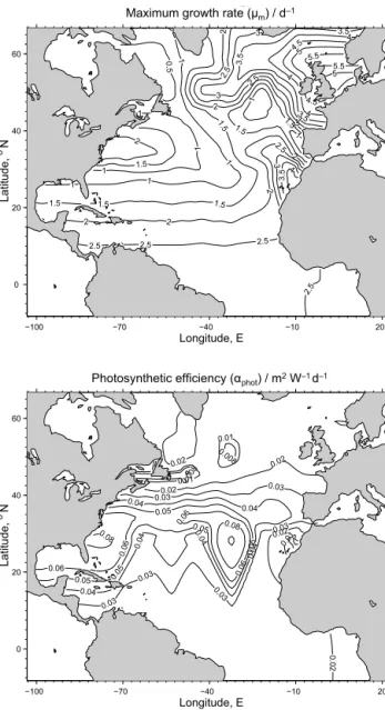
3.3 Photosynthesis as a function of light (P–I curve) In a P–I curve the level of increase from low to high irra- diance is specified by the initial slope parameter (the maxi- mum of the first derivative of the P–I curve with respect to light), also referred to as photosynthetic efficiency (αphot) (Smith, 1936; Jassby and Platt, 1976; Cullen et al., 1992;
Baumert, 1996). Photosynthetic efficiencies were derived from P–I measurements, for example by Platt and Jassby (1976), Peterson et al. (1987), and Platt et al. (1992), and their mean values were used for many N-based models (e.g.
Fasham et al., 1990; Sarmiento et al., 1993; Doney et al., 1996; Oschlies and Garçon, 1999). Published measurements ofαphotwere typically normalized to Chlaconcentrations. In case of N- or P-based models careful considerations are then needed with respect to the phytoplankton’s cellular Chl a content, which can vary by a factor of 10 and more. Val- ues ofαphot were found to vary by a factor of 3 (Côté and Platt, 1983) during a 3-month period, which can be attributed to changes in phytoplankton community structure as well
as to photo-acclimation. Platt and Jassby (1976) reported an even larger variational range over a 1-year period, from αphot=0.03 to 0.63 mg C (mg Chl a)−1h−1W−1m2 within the upper 10 m.
3.4 Algal growth and nutrient limitation
Typical parameterizations of growth limitation by nutrient availability (ambient nutrient concentrations) are expressed with the half-saturation constant (Ks) of a classical Monod equation (Monod, 1942, 1949). Another approach is to pa- rameterize limitations of the nutrient uptake rate, described with a parameter referred to as nutrient affinity (αaff) (Ak- snes and Egge, 1991). The affinity-based parameterization may also be applied to describe nutrient-limited growth, as- suming that the rates of nutrient uptake and growth are bal- anced. In this case both parameters (Ksandαaff) can be in- terpreted as being interrelated:αaff=µm·fT/Ks. However, αaffis derived from mechanistic considerations that are fun- damentally different from former interpretations ofKs of a Monod equation (Pahlow, 2005; Armstrong, 2008; Pahlow and Oschlies, 2013; Fiksen et al., 2013). For comparison between estimates ofαaff it is important to know whether this parameter describes limitation of growth or of nutrient uptake. The description of nutrient limited growth with the Monod equation, thereby retrieving values forKsfrom mea- surements, had been discussed in the past (e.g. Eppley et al., 1969; Falkowski, 1975; Burmaster, 1979; Droop, 1983). This discussion regained attention during recent years and the sole application of the Monod equation is currently viewed as a considerable drawback when simulating plankton growth un- der transient (unbalanced growth) conditions (Flynn, 2003;
Smith et al., 2009, 2014, 2015; Franks, 2009).
3.5 Algal growth and intracellular acclimation
More complex growth dependencies are described with models that consider intracellular acclimation dynamics (e.g. Geider et al., 1998; Pahlow, 2005; Armstrong, 2008;
Wirtz and Pahlow, 2010). In these models, photoautotrophic growth rates become dependent on cell quota, e.g. usually normalized to carbon biomass (N : C), and the amount of syn- thesized Chlaper cell. With such approaches, the changes in the mass distribution of phytoplankton C and N, as well as the cellular Chla content, have to be explicitly resolved in the model. One advantage is that these models are more sen- sitive to variations in light conditions and nutrient availabil- ity. The respective equations involve physiological parame- ters that are related but not identical to those of classical N- or P-based growth models, which impedes a direct comparison of older estimates of growth parameters with values currently used in models with acclimation processes resolved.
3.6 Losses of phytoplankton biomass
Parameterizations of phytoplankton cell losses involve lysis (starvation and/or viral infection), the aggregation of cells to- gether with all other suspended matter, and grazing by zoo- plankton. Exudation and leakage are processes of organic matter loss that occur while the physiology of the algae is functional. Cell lysis, exudation, and leakage are usually ex- pressed as a single rate parameter and this loss of organic matter is assumed to be proportional to the phytoplankton biomass.
Parameterizations of phytoplankton losses due to the pro- cess of coagulation and sinking of phytoplankton and detri- tal aggregates are basically derived from the principle the- ory of coagulation. The application of coagulation theory to simulate phytoplankton aggregation is well established for models that resolve size classes of particles (of phytoplank- ton cells and detritus) explicitly (Jackson, 1990). But the rep- resentativeness of simplifications (e.g. reduction to two size classes) assumed for model simulations remains an open task (e.g. Ruiz et al., 2002; Burd and Jackson, 2009). Aggrega- tion parameters in marine ecosystem models are often as- sumed to represent the combination of a collision rate and the probability of two particles sticking together after collision (e.g. stickiness of algal cells). These two parameters, colli- sion rate and stickiness, are multiplied by each other to yield a final aggregation rate. They are therefore difficult to esti- mate separately. Unless prior information can be used their estimates are always collinear, which suggests estimation of their product instead (as done in the example in Sect. 5.4).
A common problem is to find constraints that allow for a clear distinction between phytoplankton losses due to the export of aggregated cells and the loss because of grazing.
Both processes can be responsible for the drawdown of phy- toplankton biomass, and data that cover the onset, peak, and decline of a bloom are needed for a possible distinction. How the complex nature of predator–prey interaction is parameter- ized remains a critical element of plankton ecosystem mod- els. Compared to the approaches that describe algal growth, an even larger number of different parameterizations exist for grazing (Gentleman et al., 2003). Experimental data of graz- ing rates and collections of field data of zooplankton abun- dance are therefore of great value.
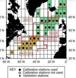
Elaborate analyses of mesozooplankton and microzoo- plankton biomass, grazing, and mortality rates were done by Buitenhuis et al. (2006, 2010). For their two studies they compiled an extensive database with laboratory and field measurements. With their data syntheses they could derive parameter values for simulations with a global ocean bio- geochemical model. Furthermore, independent field data, not used to derive the mesozooplankton and microzooplankton parameter values, were considered for assessing the perfor- mance of their model on a global scale. Their work reflects the large effort that can be dedicated to this topic for achiev- ing reliable simulation results of zooplankton grazing.
The explicit distinction between zooplankton size classes, like mesozooplankton and microzooplankton, was bypassed in Pahlow et al. (2008). Their model allows for omnivory within the zooplankton community, which is resolved by in- troducing adaptive food preferences. These preferences are treated as trait (property) state variables that adapt to the rel- ative availability of different prey. This reduces the number of parameters needed to describe a variety of different be- haviours in grazing responses. Field data from three ocean sites in the North Atlantic were used by Pahlow et al. (2008) for calibrating their plankton model. They conducted a two- step approach for parameter optimization. First they opti- mized parameter values so that depths and dates of minimum and maximum observed values become well represented by their model at all three sites. In a second step they refined their parameter estimates by minimizing weighted data–
model residuals. After parameter optimization they identi- fied distinctive complex patterns between zooplankton graz- ing and plankton composition for the three simulated ocean sites. Besides their phytoplankton grazing losses it turned out that their optimal estimates of photo-acclimation and maxi- mum C-fixation (αphot,PmC) agree with those values derived from model calibrations with laboratory data.
3.7 Constraining simulations of algal growth with laboratory and mesocosm data
Parameter values of acclimation models have typically been adjusted to explain laboratory measurements (Geider et al., 1998; Flynn et al., 2001; Pahlow, 2005; Armstrong, 2006;
Smith and Yamanaka, 2007a; Pahlow and Oschlies, 2009;
Wirtz and Pahlow, 2010). So far, there is a limited number of experimental studies whose data were used to calibrate these acclimation models (Laws and Bannister, 1980; Terry et al., 1983, 1985; Healey, 1985; Flynn et al., 1994; Anning et al., 2000). Model calibrations were usually done by tuning parameter values so that model solutions provide a qualita- tive good fit to the laboratory data. In many cases the param- eter adjustments relied on the researchers’ experience and intuition, sometimes accounting for prior parameter values obtained from preceding model analyses (e.g. Flynn et al., 2001). Analyses of parameter uncertainties of recent accli- mation models are often lacking. Most laboratory modelling studies had put emphasis on the physiological mechanistic model behaviour, while error assumptions for quantitative data–model comparison were hardly considered.
Explicit error assumptions for parameter optimizations and for comparisons of acclimation model results with lab- oratory data were introduced by Armstrong (2006) and by Smith and Yamanaka (2007a). In both studies additive un- correlated Gaussian observational errors were assumed and optimized results of different model versions had been com- pared. Armstrong (2006) applied a simulated annealing al- gorithm (Metropolis et al., 1953) to fit his optimality-based model version to the data of Laws and Bannister (1980). The
same data were used to also fit the model of Geider et al.
(1998), and he evaluated the likelihood ratio of the two ML estimates, to discuss and underpin the improved performance of his refined acclimation parameterizations. Smith and Ya- manaka (2007a) also compared the performance of two ac- climation models, of Geider et al. (1998) and Pahlow (2005) respectively. Optimal parameter values for the two model versions were obtained with the MCMC method, minimiz- ing the misfit between model results and data of the Flynn et al. (1994) experiment. Apart from mechanistic considera- tions, Smith and Yamanaka (2007a) concluded that the mod- els of Pahlow (2005) and Geider et al. (1998) described the assimilated data equally well, since both cost function mini- mum values were comparable. However, the simulated N : C and Chla: N ratios of the model proposed by Pahlow (2005) were in much better agreement with observations during the exponential growth phase, which remained undifferentiated by their error model (assuming C, N, and Chla data to be independent). Different considerations for error models will be addressed hereafter in Sect. 4.
To collect diverse data that fully resolve onset, peak and decline of an algal bloom at ocean sites is difficult to achieve.
Data derived from remote sensing, e.g. Chla concentration and primary production rates, provide limited information to explain relevant differences between processes described be- fore, like N-utilization, fixation and release of C, and syn- thesis and degradation of Chla. Mesocosm experiments that enclose a large volume of a natural plankton and microbial community can be helpful in this respect, if they provide a good temporal resolution of the exponential growth phase as well as of the post-bloom period. Vallino (2000) highlighted the benefits of using mesocosm data to test plankton ecosys- tem models, as done before by Baretta-Bekker et al. (1994, 1998). One advantage is that mesocosms are, apart from the surface, closed systems and measurements of inorganic nu- trients, dissolved and particulate organic matter should, in principle, add up to approximately constant concentrations of total nitrogen and total phosphorus. Total carbon concen- trations may only vary due to air–sea gas exchange. By de- sign these experiments often integrate valuable series of joint and parallel measurements, yielding detailed data from vari- ous scientist with different expertise (e.g. Williams and Egge, 1998; Riebesell et al., 2008; Guieu et al., 2014). Drawbacks are uncertainties in initial conditions and also the representa- tiveness of mesocosm data to reflect the real dynamics in the ocean is subject to discussion (e.g. Watts and Bigg, 2001).
In spite of these limitations, simulations of mesocosms or of enclosures experiments (e.g. with large carboys deployed in the field) have helped to identify credible model parame- ter values and assess model performance. This is particularly true for tracing microbial dynamics (Van den Meersche et al., 2004; Lignell et al., 2013) or for details in the composition and fate of particulate organic carbon and nitrogen (POC and PON) (Schartau et al., 2007; Joassin et al., 2011).
In contrast to laboratory measurements, data from meso- cosm experiments reflect some natural variability of the plankton community, mainly captured by replicate meso- cosms. The availability of measurements from replicate mesocosms is also helpful when defining error models that specify the statistical treatment of the data used for parame- ter estimation.
4 Error models
Error models define our assumptions about uncertainties and the statistical relationships between observed data, the true state, model output, model inputs (forcings and ini- tial/boundary conditions), and model parameters. Here we review error models that have been applied to address the various sources of uncertainty in marine ecosystem models and consider their implications for parameter identification.
An explicit treatment of each source of uncertainty may not be necessary, but we do recommend reflecting on how these uncertainties can be accounted for when modelling plankton dynamics and biogeochemical cycles.
4.1 Uncertainty in observations
The simplest and most common models for observational er- ror assume that the observational errorsare (i) additive nor- mal, (ii) constant variance between samples, and (iii) inde- pendent between samples and variable types. Such models are also commonly used to represent aggregated errors ac- counting for both observational and kinematic model error (see Sect. 2.1); we will refer to these asresidualerrors.
The additive normal assumption (i) is straightforward but also restricted, as it does not capture three common charac- teristics of some ecosystem data such as Chl a concentra- tions: (1) larger values tend to have larger errors, (2) values cannot be negative, and (3) the error distribution has positive skew. Characteristic (1) may be captured by scaling the stan- dard error with modelled values (e.g. Hurtt and Armstrong, 1996) or with observed values (e.g. Harmon and Challenor, 1997), while characteristic (2) can be resolved using trun- cated error distributions (e.g. Hooten et al., 2011). All three characteristics together can be captured by gamma distribu- tions (Dowd, 2007) or power-normal distributions whereby normality is assumed on a power-transformed scale (Free- man and Modarres, 2006). The power-normal family in- cludes lognormal (e.g. Hemmings et al., 2003) and square- root normal models (e.g. Fasham and Evans, 1995).
For power-normal, gamma, or proportional error assump- tions we have the difficulty that the variance on the original scale approaches zero at low values. This may be unrealis- tic, at least in regard to instrumental noise. In normal models this problem can be addressed by adding a constant term to the variance (Schartau et al., 2001; Schartau and Oschlies, 2003) or standard deviation (Vallino, 2000). Another diffi-