Probabilistic approaches to hydrological and herbicide transport modelling: Using deterministic and stochastic models to assess diffuse herbicide pollution of a headwater catchment caused by fast transport processes

Research Collection

Doctoral Thesis

Probabilistic approaches to hydrological and herbicide transport modelling

Using deterministic and stochastic models to assess diffuse herbicide pollution of a headwater catchment caused by fast transport processes

Author(s):

Ammann, Lorenz Publication Date:

2020

Permanent Link:

https://doi.org/10.3929/ethz-b-000430719

Rights / License:

In Copyright - Non-Commercial Use Permitted

This page was generated automatically upon download from the ETH Zurich Research Collection. For more information please consult the Terms of use.

Probabilistic approaches to hydrological and herbicide transport modelling

Using deterministic and stochastic models to assess diffuse herbicide pollution of a headwater catchment caused by fast

transport processes

A thesis submitted to attain the degree of DOCTOR OF SCIENCES of ETH ZURICH

(Dr. sc. ETH Zurich)

presented by LORENZ AMMANN

MSc ETH Env Eng, Swiss Federal Institute of Technology (ETH Zurich) BSc ETH Env Eng, Swiss Federal Institute of Technology (ETH Zurich)

born on 09.05.1989 citizen of M¨annedorf ZH

accepted on the recommendation of Prof. Dr. Peter Reichert, examiner Dr. Fabrizio Fenicia, co-examiner Dr. Christian Stamm, co-examiner Prof. Dr. Paolo Burlando, co-examiner

Prof. Dr. rer.nat. Dr.-Ing. Andr´as B´ardossy, co-examiner

2020

Due to growing global population and changes in lifestyle, anthropogenic pres- sure on water resources has been increasing in the last decades. Micropollutants are recognized as an increasingly important class of compounds that affect water quality. A significant part of the pollution risk originating from micropollutants is caused by pesticides that enter the natural environment through agricultural prac- tices. In particular, streams in small headwater catchments are at risk of high pes- ticide concentrations caused by fast transport during precipitation events. A good quantitative assessment of the short-term peak concentrations and the relevant flow paths that are causing them is needed. This is difficult to achieve due to the high spatio-temporal variability of the processes and the high cost of related measure- ment campaigns, which makes models a valuable complementary tool. Since models are hypotheses about the behaviour of systems, we can learn by testing different models against observations. In this regard, the potential of parsimonious “concep- tual” models to describe dynamic pesticide transport at the catchment scale has not been fully explored yet. Models are inherently uncertain, but a comprehensive probabilistic assessment of their uncertainty can be difficult to achieve. Bayesian methods are promising in this respect since they allow to update prior knowledge with new observations in a coherent probabilistic framework. W.r.t. their treatment of uncertainty, models can be classified based on whether they rely on a deterministic or a stochastic representation of internal processes. In consequence, three questions arise, which are treated in the following three paragraphs: (1) can we improve the characterization of the lumped uncertainty of deterministic hydrological models?

(2) How can we build parsimonious models to assess pesticide transport, and can we, based on findings from (1), compare their agreement with data to learn about the system? (3) Can we learn about structural deficiencies and improve the realism of the uncertainty estimates of such models by exchanging a deterministic process representation for a stochastic one?

It has been shown that the residual lumped error term that is often used in com- bination with deterministic process models can have complex characteristics that tare difficult to capture. Keeping in mind the goal of quantifying the lumped uncer- tainty of dynamic pesticide transport models w.r.t high-frequency data, we design a framework for likelihood functions for deterministic hydrological models. Thereby, we combine the possibility for an arbitrary marginal probability distributions of observations, autocorrelated errors, and non-equidistant observations (as frequently encountered in flow-proportional sampling schemes). Within the framework, we test the effect of different assumptions regarding the residual error in combination with a conceptual hydrological model and high-frequency streamflow data in a Bayesian inference setting relying on an ensemble MCMC sampler. Thereby, we find that conventional ways of considering constant autocorrelation of the errors can lead to biased results, in particular for high-frequency data. We argue that autocor- relation can be time-varying due to the forcing (in this case precipitation), that temporarily destroys the memory-effect otherwise introduced upon the output by the model states. We show that relaxing the stationarity assumption of the auto-

fields. Open questions remain regarding the optimal parameterization of the time- dependent autocorrelation, as well as regarding an efficient procedure for finding realistic distributional assumptions about the errors.

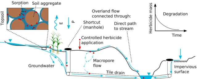
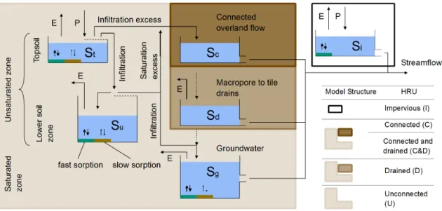
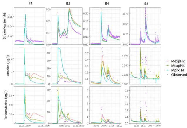
Conceptual models are a promising tool to assess the fast transport of pesti- cides in small catchments, since they balance the ability to incorporate process understanding with the need to limit model complexity in terms of computational requirements and number of calibration parameters. Limited guidance is available on their construction, even for purely hydrological applications. Our modelling approach is based on data and knowledge obtained in a previously conducted con- trolled herbicide application experiment in a small agricultural catchment typical for the Swiss Plateau. We take a systematic approach to building conceptual models for this system, transparently communicating individual modelling decisions, which are guided by experimentalists’ knowledge, as well as modellers’ experience. Us- ing a Bayesian approach, the developed models are calibrated to observations of streamflow, two herbicides, and soil/water distribution coefficients. Facilitated by the implementation of the model in a flexible modelling framework, some critical assumptions about components of the models are compared and tested against data as multiple working hypotheses. Thereby, we find that relatively simple models based on approx. 15 parameters can lead to an accurate representation of herbicide fate in the study catchment. Furthermore, including herbicide input onto imper- vious surfaces reduces the model bias compared to the assumption of no herbicide input to impervious surfaces. This is an indication of spray drift occurring during application, which is the most likely source of input to those areas. Testing two different hypotheses regarding critical source areas controlling the pollution risk, we find that hydrological response units based on tile drains and artificial shortcuts on the soil surface (such as manholes to the drainage network) yield results that are better compatible with observed chemographs than spatial units motivated by the proximity of the stream as the dominant risk factor; the first result in a 30 % decrease in overall uncertainty compared to the latter. This supports the results of previous studies that have identified artificial shortcuts as potentially important elements contributing to the risk of diffuse pollution of headwater streams by pesti- cides. Challenges encountered include the vast simplifications that have to be made when using simple models for complex systems and the incomplete examination of the effects of all the necessary assumptions. Due to the uniqueness of the data we modelled, only a partial spatial validation of the developed models could be achieved, a full spatio-temporal validation remains to be done.

Stochastic process models are models that rely on a stochastic description of the fluxes or states within the model, as opposed to deterministic process models that combine a deterministic process representation with a stochastic error term.

Stochastic models acknowledge the apparent stochastic behaviour of complex sys- tems (the same forcing and initial states observed at an aggregated level lead to different model output) and are less susceptible to structural errors by allowing for

deficits and improving the characterization of the model’s uncertainty, we make one of the herbicide transport models described above stochastic. By making parame- ters instead of states stochastic, we naturally avoid the violation of mass balances.

Regressing the resulting temporal dynamics of the parameters against forcing data and model states, we find interesting patterns, e.g., a dependency of the release rate of the slow reservoir on its state. This is interpreted as a sustained baseflow of the catchment, which cannot be fully reproduced by the single non-linear reservoir that is responsible for the slow hydrological response of the model. We also find that accounting for the intrinsic stochasticity of a model leads to a more accurate distinction between the uncertainty of the true model output and its random ob- servation error, facilitating the generation of realistic model output without having to rely on a complicated parameterization of the residual error model discussed in the second paragraph. However, the inference with stochastic models proves to be challenging in this case; up to 200 model evaluations are required per iteration of the Markov Chain to achieve reasonable acceptance rates, which limits the chosen sampling methodology to very fast models. A more fundamental problem that re- mains, is the prevention of the misuse of the additional degrees of freedom resulting in overly large fluctuations of the time-dependent parameters.

Overall, this thesis contributes to an improved assessment of fast transport pro- cesses of herbicides and the resulting dynamic fluctuations of in-stream concentra- tions in a catchment that is typical for the Swiss Plateau. This is a step towards a better characterization of the overall risk posed by pesticides to aquatic ecosystems.

Potential measures to mitigate that risk, e.g. related to artificial shortcuts, can be more easily assessed in a quantitative way through the developed models. The the- sis has also contributed to the development of better methodologies for uncertainty quantification of conceptual pollutant transport models at the catchment scale and hydrological models in general, both for deterministic and stochastic process models.

Durch die wachsende Weltbev¨olkerung und einen Wandel unseres Lebensstils hat die Belastung der Wasserressourcen w¨ahrend den letzten Jahrzehnten zugenom- men. Der Einfluss von Mikroverunreinigungen r¨uckt dabei zunehmends in den Fokus des Gew¨asserschutzes. Ein bedeutender Teil des Verschmutzungspotenzials von Mi- kroverunreinigungen ist auf Pflanzenschutzmittel zur¨uckzuf¨uhren, die durch land- wirtschaftliche T¨atigkeit in die Umwelt gelangen. Besondere Gefahr droht in klei- nen B¨achen in stark landwirschaftlich genutzten Einzugsgebieten, wo durch schnel- le Transportprozesse hohe Konzentrationsspitzen verursacht werden k¨onnen. Eine Einsch¨atzung der Konzentrationsspitzen und der Transportpfade, von denen sie ver- ursacht werden, ist wichtig. Dies ist jedoch schwierig zu erreichen, da die Prozesse r¨aumlich und zeitlich sehr variabel und Messkampagnen teuer sind, was Modelle zu wertvollen erg¨anzenden Werkzeugen macht. Da Modelle Hypothesen ¨uber das Sys- temverhalten darstellen, k¨onnen wir Wissen erlangen, indem wir verschiedene Mo- delle mit Hilfe von Messungen testen. Das Potenzial von “konzeptionellen”Modellen f¨ur den Transport von Pflanzenschutzmitteln auf Einzugsgebietsskala wurde in die- ser Hinsicht noch nicht gen¨ugend erforscht. Modelle sind mit Unsicherheit behaftet, jedoch gestaltet sich eine ganzheitliche probabilistische Analyse der Unsicherheit oft schwierig. Bayessche Methoden sind in dieser Hinsicht vielversprechend, da sie es erlauben A-priori-Wahrscheinlichkeiten durch neue Beobachtungen in einem proba- bilistischen Rahmen zu aktualisieren. Hinsichtlich der Behandlung von Unsicherhei- ten kann zwischen Modellen mit einer deterministischen oder einer stochastischen Formulierung der internen Prozesse unterschieden werden (nachfolgend als deter- ministische bzw. stochastische Modelle bezeichnet). Zusammenfassend stellen sich folgende drei Fragen, die in den nachfolgenden Abschnitten behandelt werden: (1) k¨onnen wir die Beschreibung der zusammengefassten Unsicherheit von deterministi- schen hydrologischen Modellen verbessern? (2) Wie lassen sich einfache Modelle f¨ur den Transport von Pflanzenschutzmitteln erstellen, und k¨onnen wir, basierend auf Erkenntnissen in Bezug auf (1), diese Modelle untereinander vergleichen um etwas uber das System zu lernen? (3) K¨¨ onnen wir durch stochastische Modelle Einblicke in strukturelle Fehler der Modelle gewinnen und ihre Unsicherheit besser beschreiben?

Es ist bekannt, dass die Residuen von deterministischen hydrologischen Modellen oft komplexe Eigenschaften aufweisen. Hinsichtlich der Quantifizierung der Gesam- tunsicherheit von dynamischen Transportmodellen im Zusammenhang mit hochfre- quenten Messungen erstellen wir ein allgemeines Konzept f¨ur Likelihood-Funktionen f¨ur deterministische hydrologische Modelle. Dabei kombinieren wir die M¨oglichkeit einer beliebigen Marginalverteilung f¨ur die Beobachtungen, autokorrelierte Residu- en, und ungleichm¨assige Messintervalle (wie sie oft bei Abflussproportionalen Mes- sungen vorkommen). Innerhalb dieses Konzepts testen wir die Auswirkung von ver- schiedenen statistischen Annahmen bez¨uglich der Residuen eines konzeptionellen hydrologischen Modells auf die Bayessche Inferenz mit Hilfe eines Ensemble MCMC Samplers. Dabei zeigen wir, dass konventionelle Ans¨atze zur Beschreibung der kon- stanten Autokorrelation der Residuen zu systematischen Vorhersagefehlern f¨uhren, insbesondere im Zusammenhang mit hochfrequenten Messdaten. Wir postulieren,

Zustandsvariablen auf den Output haben, tempor¨ar auf. Wenn man die Annahme einer konstanten Autokorrelation der Residuen aufgibt, kann man eine bedeuten- de Reduktion der Vorhersagefehler erreichen. Das erm¨oglicht es potenziell, neue Ans¨atze f¨ur die Kalibrierung von hydrologischen Modellen auszuprobieren, eventu- ell sogar von Modellen aus anderen Fachgebieten. Ungel¨oste Probleme bestehen in Bezug auf die optimale Parametrisierung der zeitabh¨angigen Autokorrelation, sowie eine effiziente Methode, realistische Verteilungsannahmen f¨ur die Fehler zu finden.

Konzeptionelle Modelle sind ein vielversprechendes Werkzeug zur Charakterisie- rung der Transportprozesse von Pflanzenschutzmitteln in kleinen Einzugsgebieten.

Sie erm¨oglichen den Einbezug von physikalischem Prozessverst¨andnis mit relativ geringem Rechenaufwand und kleiner Anzahl an Parametern. Es sind jedoch nur begrenzte Erfahrungen zur Konstruktion solcher Modelle vorhanden, sogar f¨ur rein hydrologische Anwendungen. Unser Modellierungsansatz basiert auf Daten und Wis- sen, welches in einem vorhergehenden Experiment mit kontrollierter Applikation von Pflanzenschutzmitteln in einem kleinen, f¨ur das schweizerische Mittelland typischen, Einzugsgebiet durchgef¨uhrt wurde. Wir verfolgen einen systematischen Ansatz zur Konstruktion von konzeptionellen Modellen f¨ur dieses System, wobei wir Entschei- dungen auf Basis des Wissens von Experimentalisten und der Erfahrung von Mo- dellierern treffen und transparent kommunizieren. Mit Hilfe eines Baysschen Ansat- zes werden die entwickelten Modelle kalibriert unter Einbezug von Messungen des Abflusses, zwei Herbiziden und Boden-Wasser-Verteilungskoeffizienten. Beg¨unstigt durch die Implementierung mit einer flexiblen Modellierungssoftware, vergleichen wir einige wichtige Annahmen ¨uber Komponenten der Modelle und testen diese als Arbeitshypothesen mit den erw¨ahnten Messungen. Dabei stellen wir fest, dass relativ einfache Modelle mit ca. 15 Parametern schon zu einer befriedigenden Be- schreibung der Transport- und Abbauprozesse von Pflanzenschutzmitteln im Ver- suchseinzugsgebiet f¨ahig sind. Durch die Ber¨ucksichtigung eines gewissen Eintrags an Pflanzenschutzmitteln auf befestigte Fl¨achen konnte der Modellfehler deutlich re- duziert werden im Vergleich zur gegens¨atzlichen Annahme von keinem Eintrag auf diese Fl¨achen. Dies deutet darauf hin, dass w¨ahrend der Applikation der Pflanzen- schutzmittel eine ¨Ubertragung durch die Luft auf befestigte Fl¨achen und eine Mo- bilisierung im darauffolgenden Regenereignis stattfand. Durch das Testen von zwei verschiedenen Hypothesen zu den kritischen Ursprungsfl¨achen von Pflanzenschutz- mitteln zeigen wir, dass die Einbeziehung von Elementen wie Drainagerohren und hydraulischen Kurzschl¨ussen (wie z.B. Unterhaltssch¨achte) zu Resultaten f¨uhren, die eher kompatibel sind mit den Messungen als die g¨angigere Annahme der N¨ahe zum Gew¨asser als dominanter Risikofaktor. Das Modell, das ersterem Ansatz folgt, resultiert in einer um 30 % reduzierten Unsicherheit im Vergleich zur letzterem. Dies best¨atigt die Resultate fr¨uherer Studien, die hydraulische Kurzschl¨usse als Elemente identifizierte, die potenziell wichtig sind f¨ur die Einsch¨atzung des Verschmutzungs- risikos, das von Pflanzenschutzmitteln in kleinen Einzugsgebieten ausgeht. Was ei- ne Herausforderung bleibt, sind die starken Vereinfachungen, die gemacht werden

Einmaligkeit des untersuchten Datensatzes konnte nur eine unvollst¨andige r¨aumliche Validierung durchgef¨uhrt werden; eine weitergehende zeitliche und r¨aumliche Vali- dierung bleibt noch offen.

Stochastische Prozessmodelle kombinieren nicht einfach eine deterministische Beschreibung der internen Prozesse mit einem stochastischen Fehlerterm, sie be- schreiben die internen Prozesse auf stochastische Art und Weise. Dadurch tragen sie dem scheinbar stochastischen Verhalten von komplexen Systemen Rechnung (die scheinbar gleichen beobachteten Rahmenbedingungen und Anfangszust¨ande f¨uhren zu unterschiedlichen Ergebnissen). Sie sind auch weniger anf¨allig auf strukturel- le Fehler, da sie unterschiedliche Entwicklungen der Zustandsgr¨ossen f¨ur dieselbe Kombination von Input und Parameter zulassen. Wir machen eines der oben be- schriebenen Transportmodelle stochastisch, um das Potenzial von stochastischen Prozessmodellen hinsichtlich der Aufdeckung von strukturellen Modellfehlern sowie der Unsicherheitsquantifizierung besser absch¨atzen zu k¨onnen. Indem wir die Para- meter und nicht die Zustandsvariabeln des Modells stochastisch machen, verhindern wir die Verletzung von Massebilanzen. Nachdem wir den gesch¨atzten Zeitverlauf der Parameter in Bezug setzen zu externen Einflussgr¨ossen sowie internen Zustands- variabeln, finden wir interessante Muster wie z.B. eine Abh¨angigkeit zwischen der Ausflusskonstante des langsamen Reservoirs und seinem Wasserstand. Dies inter- pretieren wir als stabilen Basisabfluss, der nicht vollst¨andig reproduziert werden kann durch das einzelne nichtlineare Reservoir, das im Modell f¨ur den langsamen Teil der Reaktion des Einzugsgebiets vorgesehen ist. Wir stellen ebenfalls fest, dass stochastische Prozessmodelle eine bessere Unterscheidung zwischen der Unsicherheit des wahren Modelloutputs und derjenigen des zuf¨alligen Teils des Beobachtungsfeh- lers erlauben. Dies vereinfacht die Erzeugung von realistischem Modelloutput ohne auf komplizierte Parametrisierungen der Residuen (siehe zweiter Paragraph) ange- wiesen zu sein. Die Inferenz mit stochastischen Prozessmodellen bleibt jedoch eine Herausforderung: bis zu 200 Modellevaluationen waren in unserem Fall f¨ur einen Iterationsschritt der Markov-Kette n¨otig, um eine angemessene Akzeptanzrate zu erreichen, wodurch das gew¨ahlte Verfahren auf wenig rechenintensive Modelle be- schr¨ankt ist. Ein grundlegenderes Problem ist das Verhindern der missbr¨auchlichen Verwendung der zus¨atzlichen Freiheitsgrade, die zu unrealistisch grossen Schwan- kungen der zeitabh¨angigen Parameter f¨uhren k¨onnen.

Diese Arbeit tr¨agt zu einer verbesserten Beschreibung von schnellen Transport- prozessen von Pflanzenschutzmitteln und den resultierenden zeitlichen Schwankun- gen ihrer Konzentrationen in kleinen B¨achen des schweizerischen Mittellandes bei.

Dies ist ein Schritt in Richtung einer genaueren Einsch¨atzung des generellen Risikos, das Pflanzenschutzmittel f¨ur aquatische Oekosysteme darstellen. Die Auswirkung von Massnahmen zur Reduktion des Risikos, zum Beispiel in Bezug auf hydraulische Kurzschl¨usse, k¨onnen durch die entwickelten Modelle potenziell besser quantifiziert werden. Diese Arbeit tr¨agt auch zur Entwicklung von Methoden f¨ur eine bessere Unsicherheitsabsch¨atzung von konzeptionellen Schadstofftransport- sowie hydrolo-

1 Introduction 15 1.1 Pollution of headwater streams through fast transport of pesticides:

background and motivation . . . 15

1.2 Models . . . 18

1.2.1 Empirical, physically based, and conceptual models . . . 18

1.2.2 Spatial discretization . . . 20

1.2.3 Multimodel frameworks and hypothesis testing . . . 21

1.2.4 Uncertainty quantification . . . 21

1.3 Objectives of the thesis . . . 27

1.4 Structure of the thesis . . . 28

2 A likelihood framework for deterministic hydrological models and the importance of non-stationary autocorrelation 29 2.1 Introduction . . . 31

2.2 Methods . . . 36

2.2.1 Probabilistic framework . . . 36

2.2.2 Error Models . . . 39

2.2.3 Inference and prediction . . . 41

2.2.4 Evaluation criteria . . . 42

2.3 Case study setup . . . 45

2.3.2 Deterministic Hydrological Model . . . 46

2.3.3 Priors . . . 47

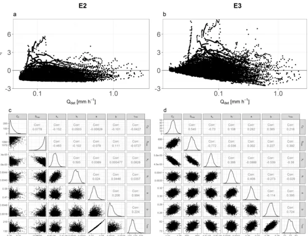
2.4 Results . . . 49

2.5 Discussion . . . 58

2.6 Conclusions . . . 63

Appendices 66 2.A Derivation of the likelihood function . . . 66

2.B Complete results . . . 67

2.C Specific error models . . . 70

2.C.1 Normal distribution . . . 70

2.C.2 Student’st-distribution . . . 70

2.C.3 Skewed Student’st-distribution . . . 71

2.D Notation . . . 73

3 Characterizing fast herbicide transport in a small agricultural catch- ment with conceptual models 75 3.1 Introduction . . . 77

3.2 Study Site and Data . . . 81

3.3 Methods . . . 83

3.3.1 Perceptual model . . . 83

3.3.2 Deterministic conceptual models . . . 84

3.3.3 Uncertainty assessment . . . 92

3.3.4 Performance evaluation . . . 94

3.4 Results . . . 95

3.4.1 Model comparison . . . 95

3.5 Discussion . . . 101

3.5.1 Model building and inference . . . 101

3.5.2 Model comparison . . . 101

3.5.3 Uncertainty and extrapolation . . . 102

3.5.4 Methodological pitfalls . . . 102

3.6 Conclusions . . . 104

4 Quantifying the uncertainty of a conceptual herbicide transport model with time-dependent, stochastic parameters 107 4.1 Introduction . . . 109

4.2 Methods . . . 113

4.2.1 Study site and data . . . 113

4.2.2 Probabilistic model based on time-dependent parameters . . . 113

4.2.3 Finding patterns with local regression and cross-correlation . . 115

4.2.4 Model improvement based on patterns found in time-dependent parameters . . . 118

4.2.5 Prediction . . . 118

4.2.6 Numerical implementation of model and sampler . . . 119

4.3 Results and Discussion . . . 121

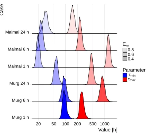
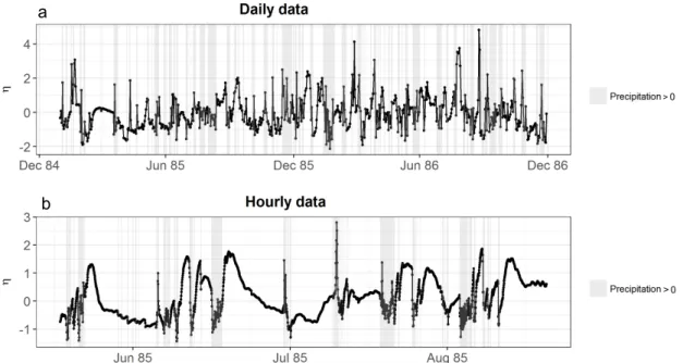
4.3.1 Inferred dynamics of time-dependent parameters and identi- fied patterns . . . 121

4.3.2 Model improvement by incorporating found patterns . . . 129

4.3.3 Estimated uncertainties based on Bayesian posterior distribu- tions . . . 129

4.4 Conclusions . . . 133

Appendices 136

4.B Temporal dynamics and predictive uncertainty obtained for time-

dependent S_t,z2 . . . 139

4.C Additional results . . . 142

5 Conclusions and outlook 145 5.1 Conclusions of the main chapters . . . 146

5.1.1 Characterization of the additive error for deterministic process models . . . 146

5.1.2 Assessing fast herbicide transport in headwater catchments . . 147

5.1.3 Application of stochastic process models for questions of water quality . . . 148

5.2 Overall conclusions . . . 149

5.3 Suggestions for further research . . . 150

6 Supporting information to Chapter 2 173 6.1 Synthetic case study: inferring known true parameters . . . 173

6.2 Complete results . . . 175

6.2.1 Marginal prior and posterior densities . . . 175

6.2.2 Kullback-Leibler divergence . . . 182

6.2.3 Standardized innovations . . . 185

7 Supporting information to Chapter 3 186 7.1 Data pre-processing . . . 186

7.2 Modelling sorption and degradation in SUPERFLEX . . . 188

7.2.1 Literature review . . . 188

7.2.2 Modelling sorption and degradation with partially mixed reser- voirs . . . 188

7.3 Model structures and equations . . . 191

7.5 Likelihood function and prediction . . . 196

7.6 Performance metrics . . . 198

7.6.1 Reliability . . . 198

7.6.2 Relative spread . . . 198

7.7 Herbicide inputs to HRUs . . . 199

7.8 Performance metrics of all models . . . 200

7.9 Prior and posterior parameter distribution . . . 201

7.10 States and fluxes of the reference model . . . 209

8 Supporting information to Chapter 4 217 8.1 Inferred temporal dynamics and predictive uncertainty achieved with all instances of time-dependent parameters . . . 217

8.2 Comparison of marginal posteriors of constant parameters . . . 240

8.3 Comparison of marginal posteriors when using single and multiple time-dependent parameters . . . 241

8.4 Comparison of inference results when fitting only streamflow and when fitting full data . . . 247

There are many people who greatly supported this work in various different ways.

I am extremely grateful for all this support and I will try to appropriately express this gratitude in the following paragraphs.

First of all, I would like to highlight the great direct scientific support that I received from my supervisors throughout the whole project. Peter Reichert sup- ported this work in uncountable ways with his exceptional dedication and passion.

He taught me the value of critical and precise thinking among many other things.

To Fabrizio Fenicia, I am especially grateful for his relentless support and patience, and for introducing me to the art of scientific reasoning and writing clearly struc- tured papers. I would also like to express my appreciation to Christian Stamm and Tobias Doppler for their valuable inputs to this project at multiple stages. I also appreciate the helpful ideas and comments of Paolo Burlando and Andr´as B´ardossy in their role as co-examiners during the project.

Many more people have contributed to this work scientifically in a direct or indirect way through comments, feedback, discussions and by providing inspiration.

In this regard, I want to explicitly thank Reynold Chow, Carlo Albert, Omar Wani, Andreas Scheidegger, Dmitri Kavetski, Nele Schuwirth, Marco dal Molin, Bogdan Caradima, Volker Prasuhn, Sebastian Stoll, Ruth Scheidegger, Marco Baity Jesi, Rosi Siber, and all the others who have inspired me and whom I forgot to mention here. In general, I want to thank all of the Siam department of Eawag for the great and inspiring atmosphere, which considerably facilitated conducting scientific work.

This dissertation was made possible through the funding provided by the Swiss National Science Foundation (SNF).

I also want to thank the following organizations for providing the data needed to conduct the work for this thesis: MeteoSwiss, swisstopo, WSL, and the municipality of Ossingen. I am also happy to acknowledge the outstanding administrative support provided by Karin Ghilardi, the Lib4ri-Team, the HR department of Eawag, and ETH Zurich.

A very special thanks goes to my friends and family, who supported me during every part of this journey.

Introduction

1.1 Pollution of headwater streams through fast transport of pesticides: background and mo- tivation

Water resources are an essential component of our natural environment; any pros- pering society critically relies on the availability of water of sufficient quantity and quality. As the global population increases and lifestyle changes, the anthropogenic pressure on water resources has been increasing, in particular throughout the last century. One of the most important factors driving the pressure on quantity and quality of water resources has been agricultural production. The global demand for agricultural products, expressed in monetary terms, has roughly quadrupled be- tween 1960 and 2012 [FAO, 2018]. The same study projects a further growth of ca.

50% by 2050. The main drivers for this increase have been the global population growth, as well as changes in the average diet, which in turn are related to economic growth [FAO, 2018]. One of the pillars of the increase in the agricultural output that has accompanied the elevated demand, is the development and application of vari- ous types of plant-protection products (PPP, or pesticides). Reducing the damage dealt to crops by pests, these products have supported the spread of mono-cultures as a labour-efficient way of producing food for humans and animal feed. The global crop pesticide market volume was estimated to $33 billion in 2007 [Epstein, 2014].

For 2017, global pesticide sales were projected to amount to approx. $68.5 billion [Epstein, 2014]. Global sales of herbicides, which is a subgroup of pesticides tar- geting unwanted plants, have grown from $14 billion in the year 2000 to $23 billion in 2016 [Nishimoto, 2019]. In the European Union, yearly total sales of pesticides stayed relatively constant during the period from 2011-2017 [Eurostat, 2019]. In Switzerland, the total mass of sold herbicides has decreased from approx. 850 to 600 tons between 2008 and 2017 [BLW, 2019], as opposed to the substances with

“elevated risk potential”, the sales of which have been rather constant during that

time [BLW, 2019].

In addition to their undisputed utility in facilitating crop production, some PPP and their transformation products are known to have unintended effects on non- target organisms in the biotic environment due to their very purpose of being bi- ologically active. A thoroughly compiled overview of studies on the effects of pes- ticides on non-target species can be found in Kohler and Triebskorn [2013]. Mnif et al. [2011] give an overview of the research on adverse effects of endocrine disrup- tor pesticides on human health in particular. Independent of the current state of knowledge about the actual environmental risk, persistent and mobile substances are especially unwanted in the natural environment.

In Switzerland, PPP and their transformation products are found in both, ground- water [e.g. BAFU, 2019] and surface water bodies [e.g. Spycher et al., 2018] and are known to originate mainly from agricultural practices. Pollution risks arise from individual compounds, as well as from mixtures of substances. While surface water bodies are mainly affected by parent compounds, the risk of groundwater pollution is driven by transformation products [BAFU, 2019] due to the half-life time in the order of 5 - 50 days [Lewis et al., 2016] for many frequently used active ingredients.

This thesis focuses on the transport of herbicide parent compounds from arable land to surface water bodies, in particular small headwater streams. For this purpose, transformation of the parent compounds is simply considered as degradation, and transformation products are not considered.

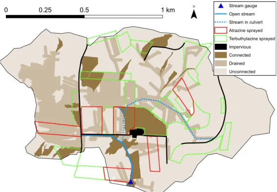
As headwater streams we understand perennial streams of one of the first few orders according to [Strahler, 1952], that are often the first permanent water bodies reached by overland flow processes. It has been estimated that ca. 80 % of the global river network consists of streams of 0-2^nd order [Downing et al., 2012]. This value is believed to be similar for European conditions [Kristensen and Globevnik, 2014]. Regarding Switzerland, Figure 1.1 reveals that the total length of the Swiss river network is dominated by streams that are less than 3 meters wide. Apart from being abundant, small waterbodies are an important pillar of freshwater biodiversity and ecosystem functioning [Biggs et al., 2017], in part because they show a large γ-diversity [Clarke et al., 2008]. An overview of the vast number of studies investi- gating the importance of headwater streams for biodiversity is provided by Meyer et al. [2007] and by Finn et al. [2011].

In headwater streams located in agricultural catchments, herbicide concentra- tions are known to vary strongly in time [e.g. Spycher et al., 2018, Doppler et al., 2012, Meyer et al., 2010]. Peak concentrations caused by rain events are likely to dominate the pesticide mass exported to small streams in humid regions [e.g. Leu et al., 2010]. Consequently, the risk posed to aquatic organisms can only be reliably assessed when taking into account the high-frequency dynamics of chemographs in such streams. Several measurement campaigns have been conducted in this direction [e.g. Leu et al., 2004, Doppler et al., 2012, Petersen et al., 2012]. Since such cam- paigns are very cost-intensive, models are useful tools to interpret and predict the

Figure 1.1: Total cumulative length of the Swiss river network as a function of river width. The river width was estimated by Rosi Siber based on a combination of the average measured river width of a sample of reaches [Zeh Weissmann et al., 2009]

for each stream order class [BAFU, 2013], which is available for the whole network according to Strahler [1952, 1957].

behaviour of small catchments by interpolating or extrapolating the collected obser- vations. Models can provide (i) quantitative estimates of the exposure of headwater streams to pesticides, (ii) assess the effectiveness of proposed mitigation measures, and (iii) provide relevant information to increase the efficiency of future measure- ment campaigns.

1.2 Models

The increasing stress on water resources mentioned in Sect. 1.1 poses new require- ments in terms of our ability to manage water related systems in a way that benefits human society to the maximal degree possible and minimizes the risk of (irreversible) damage dealt to the natural environment. Very broadly speaking, there are two fun- damental interests that we can have with respect to a certain complex environmental system: (i) understanding of the system and (ii) prediction of the behaviour of the system and its potential response to management alternatives. The first is usually a central goal in science, while the latter is very common in operational and practical settings. They are not completely independent, though, and one may hope that (i) facilitates (ii) [e.g. Kirchner, 2006], although (ii) can also be achieved without (i).

Since there is no prediction without a model, models are a prerequisite for (ii), i.e.

they are the basis to take well-informed decisions in managing environmental sys- tems to accommodate societal and environmental needs. Models can also contribute to (i) when they are used to represent hypotheses that are tested against observa- tions (see Sect. 1.2.3). Computers have been used more and more to implement complex models that surpass the capacity of the human brain in some aspects like memory.

Models of environmental systems differ in various characteristics, like number of parameters, linearity, spatial and temporal resolution, numerical implementation, etc. Various types of modelling approaches have been used to characterize the transport and export of pesticides in agricultural catchments. In the following, we give a brief overview of previous approaches sorted according to the way in which they represent the processes (Sect. 1.2.1), the way they are discretized spatially (Sect. 1.2.2), and the way they deal with uncertainty and parameter estimation (Sect. 1.2.4).

1.2.1 Empirical, physically based, and conceptual models

Regarding the type of process representation of hydrological models, a distinction that is frequently made is between empirical models, physically based models, and conceptual models. Models of the first type rely on relatively simple and partially empirical relationships to quantify the amount of exported pollutants or risk of pollution based on some explanatory variables, which are mostly chosen based on

mechanistic considerations. These models are characterized by a relatively small number of parameters and conceptual simplicity. For example, Siber et al. [2009]

construct a relatively simple regression model to estimate pollution risk based on the amount of fast flow occurring in catchments across Switzerland. Dabrowski et al.

[2002] predict the average loss of pesticides with a simple runoff model that includes catchment characteristics and chemical properties of pesticides. Such models are especially suitable for an efficient assessment of the relative pollution risk of different catchments. However, their ability of predicting environmental concentrations, let alone the temporal dynamics of these concentrations, is questionable. In purely hydrological modelling, there is a growing number of studies using approaches based on neural networks (see Kasiviswanathan and Sudheer [2017] for an overview). These methods have been shown to be especially promising for the “prediction in ungauged basins” problem in data-rich settings [e.g. Kratzert et al., 2019].

On the other hand, models that are largely physically based have been applied to characterize pesticide transport. The process description of these models is based on physical principles that have been well investigated at the lab scale. A funda- mental component of many physically based hydrological models is the Richards equation [Richards, 1931], which can be derived based on a combination of mass conservation and the momentum equation called Darcy’s law, yielding a non-linear (because the hydraulic conductivity is dependent on the soil moisture [e.g. Mualem, 1976]) diffusion equation for soil moisture. Such physical principles are then applied in each of a usually large number of grid elements that form a relatively fine spatial resolution of the catchment. Such models are appealing because, in theory, their parameters are measurable quantities, which alleviates the need for calibration, and spatio-temporal extrapolation is possible. An extensive overview of physically-based models applied to catchment-scale water quality problems is provided by Horn et al.

[2004]. There have been numerous more recent studies [e.g. Morselli et al., 2018, Gassmann et al., 2013, Villamizar and Brown, 2017, Renaud et al., 2008]. On the other hand, tools for tracking conservative tracers through a catchment to char- acterize transit time distributions have also been developed [Remondi et al., 2018, e.g.]. Such approaches are in principle also possible for non-conservative “tracers”

like pesticides. However, additional processes like degradation and sorption would need to be included, which would make such models considerably more complex and presumably more expensive to run. Due to their detailed process representation and high spatial resolution, physically based models often have more parameters than can be measured with reasonable effort [e.g. Mar´ın-Benito et al., 2014]. As a con- sequence, calibration is still necessary [Morselli et al., 2018, Gassmann et al., 2013, Remondi et al., 2018]. However, the calibration of highly complex models based on limited data is extremely challenging [e.g. Reggiani and Schellekens, 2005] and the “implicit upscaling premise” from small-scale physics to grid elements of those models has been questioned [Kirchner, 2006].

Conceptual models can be seen as a mixture of the empirical and the physically based models described above. They are based on a strongly simplified represen- tation of the physical processes that act at the scale of hill-slopes or catchments.

They are usually developed in a “top-down” approach [Fenicia et al., 2016], aiming to directly describe the emergent properties of these systems at a larger scale. Con- ceptual models have a long tradition in operational and scientific hydrology (for an overview see [Beven, 2012a]). Although there are numerous examples of conceptual models with a rather large number of parameters [e.g. Arnold et al., 1998], concep- tual models tend to be parsimonious (i.e., they have a good trade-off between model simplicity and process representation), which makes them suitable candidates for modelling hydrological systems. However, the potential of rather simple conceptual models as tools to assess pollution risk, in particular related to pesticide transport, has been insufficiently explored so far. Previous applications of largely conceptual models have been promising [Di Guardo et al., 1994, Pullan et al., 2016]. Jackson- Blake et al. [2017] make a strong argument for conceptual models for nutrient and sediment problems, showing that the simple conceptual model SimplyP performs as good as the much more complex INCA-P [Wade et al., 2002] in a case study in northeast Scotland. Conceptual models have recently also been used to accelerate physically based river water quality models [Keupers and Willems, 2017, Nguyen et al., 2018]. However, the construction of conceptual hydrological models is often non-systematic and ad-hoc, and seen as a result of “contemplation and discussion”

[Gupta et al., 2008]. Also pollutant transport studies at the scale of small catch- ments often lack a systematic approach to model building, in particular concerning the consideration of prior experimentalist’ knowledge and data.

1.2.2 Spatial discretization

Hydrological and chemical processes in a catchment can undoubtedly show a large spatial heterogeneity. It is therefore appealing from a scientific point of view to apply distributed models that hold the promise to account for that spatial hetero- geneity. The typical scale on which hydrological processes vary [e.g. Skøien and Bl¨oschl, 2006] is just one of the factors influencing the optimal choice of the spa- tial resolution of a model. Others include the availability of forcing data and the required resolution of the model output [e.g. Dehotin and Braud, 2008], where the latter can be influenced by the requirements of policy makers or managers in opera- tional settings. The finer the spatial discretization of a model, the higher is usually the number of parameters and the larger is the amount of data required to inform the parameters directly (i.e., in the form of observations of measurable parameters), or indirectly (i.e., through calibration of the parameters to observed model output), or both. For models containing a large number of elements such as grid cells, both of the mentioned strategies for informing parameters might be infeasible; the first due to the high cost of measurement campaigns, and the second due to the lack of iden- tifiability of model parameters, in hydrology sometimes called “equifinality” [Beven, 2006]. Semi-distributed models, on the other hand, do acknowledge the spatial het- erogeneity of the dominant processes, but try to avoid an excessively large number of elements that can lead to the problems described above. However, limiting the number of spatial elements at catchment scale often means accepting an element size

that is too large to directly apply well-established physically-based principles that have been tested at the lab scale. Therefore, the question of spatial discretization is not completely independent of the type of process representation (Sect. 1.2.1).

A detailed overview of the different types of elements that have been used as the basis of landscape discretization is provided by Dehotin and Braud [2008]. These elements include regular grids, e.g. of the MIKE-SHE model [Abbott et al., 1986], irregular grids [e.g. Vivoni et al., 2004], hillslopes [e.g. Zehe and Fl¨uhler, 2001], and hydrological response units (HRUs) [e.g. Fl¨ugel, 1995]. While highly discretized, physically-based models usually rely on regular or irregular grids [e.g. Abbott et al., 1986, Gassmann et al., 2013], semi-distributed models often make use of HRUs [e.g.

Arnold et al., 1998, Wade et al., 2002, Jackson-Blake et al., 2017]. HRUs facilitate the construction of parsimonious models by summarizing similarly-behaving areas into one model element for which only one set of model states needs to be evolved during the simulation period (if the forcing can also be assumed to be spatially constant over that area). This can lead to a high computational efficiency, while still capturing the major heterogeneities present in the catchment.

1.2.3 Multimodel frameworks and hypothesis testing

The scientific learning process is based on testing hypothesis about the functioning of the investigated system. Models can be seen as collections of hypotheses that summarize our believe about the processes occurring in natural systems. There- fore, by testing different models (i.e., hypotheses) against data, we can ideally learn about the underlying system. However, different pre-existing models usually differ in many ways such as the representation of the processes, numerical implementation and solution scheme, coupling of the surface and subsurface processes, and solvers used to integrate the differential equations [Kampf and Burges, 2007]. This hampers the scientific learning process as it precludes the possibility to uniquely identify the key element that causes one model to better agree with observed data than another.

Flexible modelling frameworks greatly facilitate the controlled model comparison and are therefore seen as an important step towards more rigid hypothesis testing in hydrolocial sciences [e.g. Fenicia et al., 2016, 2013]. However, we are not aware of applications of such frameworks for hypothesis testing through controlled compari- son of the performance of pollutant transport models at the catchment scale w.r.t.

observed data, which calls for scientific studies in that direction.

1.2.4 Uncertainty quantification

Since catchments are very complex systems, any model that attempts to describe their behaviour is necessarily a vast simplification of the true underlying system, which leads to deviations of the model from the actual system it represents. The im-

perfectness arising from these deviations is often called the “uncertainty” of a model.

It has been generally recognized that there is a scientific as well as practical need for reliable estimates of the uncertainty of hydrological rainfall-runoff models [e.g.

Wagener and Gupta, 2005]. During the last two decades or so, the number of studies investigating the characterization, quantification and reduction of the uncertainty of hydrological models has greatly increased. A comprehensive literature overview of the topic is, e.g., provided by Pechlivanidis et al. [2011], ordering previous studies according to the different sources of uncertainty they consider, the different meth- ods they use, and the different frameworks they develop / apply. In WQ modelling, uncertainty quantification has also been recognized as important [Rode et al., 2010], but is overall less advanced than for conventional hydrological rainfall-runoff models.

Very recently, the need for uncertainty quantification of fully empirical hydrological models has also been accepted. For example, Kasiviswanathan and Sudheer [2017]

provide an overview of the uncertainty quantification methods applied for artificial neural networks used as hydrological models.

The uncertainties related to hydrological and WQ models can be split into the following types according to their sources [Pechlivanidis et al., 2011]: natural uncer- tainty (which is referred to as “intrinsic stochasticity” in this thesis), data uncer- tainty (which includes measurement uncertainty of input and output), parameter uncertainty, and model structural uncertainty. The importance of those different types of uncertainties will depend on the properties of the system and the model, as well as on the type and amount of available data. In the following, we go through some fundamental concepts of how to formulate probabilistic models (Sect. 1.2.4.1) and how to update the model parameters based on observations (Sect. 1.2.4.2 and 1.2.4.3) that are largely independent of the specific application.

1.2.4.1 Probabilistic model formulation: deterministic vs stochastic pro- cess models

We argue that a very fundamental and important classification of models is the dis- tinction between deterministic and stochastic process models. Simply stated, what we mean by a DPM is a model that relies on a process representation (the core part of the model) that always leads to the same output when evaluated for the same input and parameters. Usually, the “core part” of the model represents phys- ical, biological, or chemical processes happening in environmental systems, but also completely empirical models can be seen as DPMs, e.g., simple linear regression or complex neural networks. Consider the output of a DPM, y_det(θ), which depends on the parameters θ. Regarding the notation, we use lower case variables for de- terministic values (vectors are bold) and upper case letters for stochastic variables.

Note that we usually omit the model input from the notation, as the distinction be- tween input and parameters is rather arbitrary from a statistical point of view; they are both quantities that affect the model states and output in some defined way.

The random variable representing the observations, Y_obs, is obtained by adding a

stochastic residual error, Ztot, to the output of the deterministic model:

Y_obs =y_det(θ) +Z_tot(y_det,ξ) (1.2.1a) or by h(Y_obs) =h y_det(θ))

+Z_tot(ξ) (1.2.1b) where the often encountered heteroscedasticity in the residual error [e.g. Clarke, 1973] is either accounted for through formulating the error term as a (usually in- creasing) function of the model output (Eq. 1.2.1a) [e.g. Evin et al., 2013] or through the transformation h(·) in Eq. (1.2.1b) [e.g. McInerney et al., 2017]. Even though this model has a stochastic element, Z_tot, the output of its process representation, y_det, is still deterministic, which is why we call it a DPM. The actual observations, y_obs, are then assumed to be a realization of the random variableY_obs. In this case, Z_tot incorporates the errors arising from different sources like input, model struc- ture, and measurement errors of the output. When predicting with such a model, one needs to be aware that one is predicting the observations and not the true sys- tem state. The difference between these is small in case of small measurement error of the output. If measurement uncertainty of output is large [Mcmillan et al., 2012], and if at the same time we want to predict the true and not the observed output, the measurement processes should be modelled explicitly. Similarly, if input mea- surement uncertainty [e.g. B´ardossy and Das, 2008] or model structural uncertainty [e.g. Butts et al., 2004] are large, they should be considered.

It has been claimed that deterministic process models are falsified by any con- ceivable measurement [Nearing et al., 2016]. However, a deterministic model can be interpreted as the expected state of an underlying stochastic system:

Yobs =E[Yobs] + (Yobs−E[Yobs]) (1.2.2) where E[·] is the expected value, the first term on the right-hand side is the output of the deterministic model, and the second is the model error. In that case, the de- terministic model is not falsified by any measurement. Thus, deterministic models can still be valuable tools to describe the behaviour of complex systems. Equation 1.2.2 reveals, however, that the stochastic term, Z_tot, might have complex charac- teristics since it summarizes all the deviations of the observation from the expected value. Those deviations originate from (and are cumulated over) many input and internal model states which makes their final characteristics more elusive.

Deterministic process models (DPMs) are ubiquitous in environmental research and practice, and they are often used to describe systems that actually behave stochastically. In addition, many of the previous applications of Eq. 1.2.1 are lack- ing a realistic characterization of Z_tot, which calls for improvements to the current state of research. Several studies have contributed to better characterize the het- eroscedasticity [e.g. G¨otzinger and B´ardossy, 2008, McInerney et al., 2017] and the distributional shape [e.g. Schoups and Vrugt, 2010] of Z_tot, but its autocorrelation has rarely been investigated in detail, especially when it comes to high-resolution data.

There is an alternative to Eq. (1.2.1) and (1.2.2) that avoids comparing the data and model outputs in their original space, but only compares certain signatures thereof [e.g. Kavetski et al., 2018]. Examples of hydrological signatures include flow duration curves, flashiness indices [Baker et al., 2004], and baseflow indices [e.g. Eckhardt, 2008]. This avoids the description of the complex characteristics of the deviations in the original space, but leads to a loss of information through the compression of the data during calculation of the signatures. The error model is still formulated in the original data space; which makes the likelihood in the signature space expensive to evaluate. Therefore, this approach has to be combined with numerical techniques like Approximate Bayes Computation [Diggle and Gratton, 1984, Vrugt and Sadegh, 2013, Kavetski et al., 2018], which do not require the evaluation of the likelihood function. Although this approach is promising for dealing with uncertainty in hydrological modelling, its exploration is outside the scope of this thesis.

Complex environmental systems often behave in a stochastic way at the resolu- tion at which we observe them. Spatio-temporally lumped observation of input and system states lead to an apparent stochastic behaviour (different output for same observed input). Therefore, the most realistic model of many environmental systems (and also many other types of complex systems), is a stochastic one:

Yobs(θ) =Ymod(θ) +Zmeas (1.2.3) where the observationsy_obs are assumed to be realization of the inherently stochastic model plus an observation measurement error, Zmeas. This theoretically leads to simpler characteristics of Z_meas, as long as the causes for the errors are correctly captured and reflected in the stochastic model. That, in turn, would alleviate the need for designing complex error models to describe Zmeas. Such a model also has the potential to provide information about the uncertainty of unobserved (internal) model states.

An overwhelming majority of the models previously applied to pesticide trans- port problems at the catchment scale fall into the category of DPMs. This is the case even though the catchments that such models describe are behaving clearly stochastically at the resolution we observe them. This calls for a better exploration of the utility of stochastic process models to quantify the uncertainty of catchment scale transport models, in particular related to the complex processes that facilitate fast transport of pesticides. Stochastic process models are much more common in purely hydrological settings, where they are predominantly applied in connection with a procedure called “data assimilation”. An overview of uncertainty quantifi- cation of hydrological models focusing on studies that perform data assimilation, is provided by Liu and Gupta [2007].

In many cases, some or all of the parameters θ are not known and need to be estimated based on observations y_obs, which is the topic of the following two sections. The approaches that are commonly used to do so can be split into those that, given y_obs, (i) find the optimal value of θ (see Sect. 1.2.4.2) or (ii) obtain the

full distribution of θ given the probabilistic model for Yobs (see Sect. 1.2.4.3).

1.2.4.2 Maximum likelihood estimation, single- and multi-objective cal- ibration

A straightforward concept to estimate parameters based on observations is the defi- nition of some objective measure that quantifies the goodness of fit of model output y_det(θ) to the data y_obs. This objective function is then maximized by varying θ.

Single objective calibration has a long tradition in hydrological modelling and the reader is, for example, referred to Moradkhani and Sorooshian [2008] for an overview of the traditional calibration methods used in hydrology. The most popular objec- tive functions include metrics like the Nash-Sutcliffe-Efficiency [Nash and Sutcliffe, 1970], as well as its adaptation, the Kling-Gupta-Efficiency [Gupta et al., 2009].

Alternatively, one can take a probabilistic approach and define a likelihood function that is based on the assumption of an error model, and that can also be optimized as an objective function in a procedure called maximum likelihood estimation. For some metrics like the Nash-Sutcliffe-Efficiency, one can easily find an equivalent probabilistic error model, in this case iid. normal errors. Likelihood approaches have the benefit of a probabilistic interpretation of uncertainty, which comes at the cost of making explicit assumptions about the error model.

It has been stated several decades ago that one should acknowledge that the optimization problem is inherently multi-objective [e.g. Gupta et al., 1998] and it has been argued that the exploration of the Pareto optimal solutions can be very beneficial [e.g. Efstratiadis and Koutsoyiannis, 2010]. It has also been recognized that hydrological models tend to be more robust when calibrated to different types of observations [e.g. Mroczkowski et al., 1997, Franks et al., 1999]. When modelling river water quality, we often have a naturally multi-objective setting when we want to accurately represent both, streamflow and concentration of pollutants. However, it has not been sufficiently explored how a multi-objective problem can be combined with a rigid probabilistic Bayesian approach to uncertainty assessment and inference (see Sect. 1.2.4.3). Some work in this area has been done [e.g. Talamba et al., 2010, Reichert and Schuwirth, 2012] for WQ models, but is is not yet clear whether such approaches are transferable to pesticide transport models at the catchment scale and to high-frequency data.

1.2.4.3 Obtaining the full distribution: Bayesian inference

There are two dominant interpretations of probabilities; the frequentist and the Bayesian interpretation. The frequentist interpretation of probabilities restricts their application to repeatable events only. A frequentist would argue that there is a true parameter, θ^∗, which is fixed but unknown. Since this parameter vector is not the outcome of a repeatable process, it does not make sense to assign probabilities

(or probability densities) to the values of a certain parameter vector. The major uncertainty quantification method resulting from the frequentist school of thought are confidence intervals. These are intervals constructed such that, if the process of constructing such intervals based on new data sampled from the underlying data generation process is repeated infinitely, a fraction α of those intervals would cover the true value,θ^∗, where α is called the confidence level.

The Bayesian interpretation of probabilities (see Berry [1996] for a comprehensive introduction) allows probabilities to be viewed as “plausibilities”. Therefore, we can express our believe about the true parameter vector,θ^∗ as a probability density function (in case of continuous values), p(θ). Consider the following probabilistic model for the observables and the parameters:

p(y,θ) =p(y|θ)p(θ) (1.2.4)

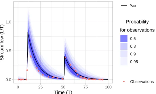
Note that the right-hand side of the equation above represents the frequently applied split of the prior into a prior for the parameters, p(θ), and a prior for the observables given the parameters, p(y|θ). This distinction is very common but rather arbitrary, since both of the terms contain prior knowledge. A typical way of designing p(y|θ) for hydrological applications is shown in Fig. 1.2. The Bayesian paradigm combines this prior believe about the data generating process with actual observed data to update our believe about the parameters:

p(θ|y_obs) = p(y_obs,θ)

p(y_obs) ∝p(y_obs,θ) (1.2.5) where p(θ|y_obs) is the posterior probability of the parameters given new obser- vations, y_obs. If the same split as in Eq. (1.2.4) is applied to the right-hand side of Eq. (1.2.5), we obtain p(y_obs|θ), or L(θ), which is often called the likelihood func- tion. This function is used for inference as a function of parameters only, keeping the observations fixed. A closed form representation of p(θ|y_obs) usually requires solving high-dimensional integrals to obtain p(y_obs), and is therefore often infeasi- ble. Obtaining a sample ofp(θ|y_obs), however, does not requirep(y_obs) to be known since the latter is constant w.r.t. the parameters. If p(y_obs,θ) is also not available in closed form, the posterior cannot be sampled directly and alternative methods (e.g. Approximate Bayes computation [e.g. Diggle and Gratton, 1984]) have to be applied. A multitude of samplers (see Robert et al. [2018] for an overview), each with its own advantages and disadvantages, can be used to sample from p(θ|y_obs) or approximations thereof. The efficiency of the different sampling techniques varies dramatically depending on the dimensionality of the distribution and its correlation structure.

Once a sample of p(θ|y_obs) has been obtained, this sample (hopefully) expresses the increased knowledge about the system obtained through the new data in the form of a narrower distribution of the parameters, the posterior distribution. With

●

●

●

●

●

●

●

●

●

●

●

●●

●

●

●

●

●

●

●

●

●

●

●

●

●

●

●

●

●

●

●●●●●

●

●

●

●

●

●

●

●

●

●

●

● ●●●●●●●●

●

●

●

●●●●● ●●●● ●●●●●●●●

●

●

●

●

●

●

●

●●●●●

●

●

●

●

●

●

●

●●●●●

●

●

●

●●●●●

●

●

●

●●●●●●●●●●●●●

●

●

●

●●●●● ●●●●●●●●●●●●●●●● ●●●●●●●●●●●● ●●●● ●●●●●●●●●●●●●●●● ●●●●

●

●

●

● ●●●● ●●●●●●●●

0.0 0.5 1.0

0 25 50 75 100

Time (T)

Streamflow (L/T)

y_det

Probability for observations

0.5 0.8 0.9 0.95

● Observations

Figure 1.2: Illustration of a probabilistic model constructed for hydrological appli- cations. The area shaded in blue denotes a hypothetical marginal probability for the observations based on a lognormal distribution that evolves in time, the mean of which is equal to y_det and the standard deviation is given by a monotonically increasing function of y_det.

the increased knowledge about the system we can make, if required, new predictions from our model by propagating the sample of p(θ|y_obs) through p(y|θ) to obtain a sample of y at the required spatial or temporal locations.

The great potential of Bayesian approaches to uncertainty quantification has been recognized in the hydrological sciences more than a decade ago. For example, Kuczera et al. [2006] introduce a Bayesian framework to account for different sources of errors explicitly. Ajami et al. [2007] perform a similar analysis, but adapt the formulation of the input error to a time-continuous multiplication factor for pre- cipitation and include model structural uncertainty. There are a number of water quality modelling studies that use formal Bayesian approaches [e.g. Raat et al., 2004, Hong et al., 2005, Talamba et al., 2010, Gardner et al., 2011, Han and Zheng, 2018], but the applicability of Bayesian approaches has not been sufficiently explored in case studies with high-resolution water quality data, in particular concentrations of pesticides.

1.3 Objectives of the thesis

The objectives of this thesis can be hierarchically arranged into the following higher- and lower-level objectives:

1. Quantitatively assess the dynamic response in streamflow and herbicide con- centrations caused by precipitation events in small headwater catchments with the help of models. Investigate the relevant processes for herbicide fate and the degree to which they contribute to a fast transport to the stream.

(a) Investigate how prior experimentalists’ knowledge can be included in the process of building models that represent the relevant processes at catch- ment scale

(b) Through model comparison, assess the performance of different model configurations that vary in the degree of complexity and the hypothesis about the dominant spatial factors controlling the risk of fast transport processes.

2. Improve the uncertainty quantification of hydrological models in general and pesticide transport models in particular

(a) Improve the quantification of the lumped uncertainty of deterministic hydrological models. Develop a framework that considers the most im- portant statistical properties of the lumped error term that are typical for hydrological and water quality problems. Test the effect of different statistical assumptions about the residual error on the inference and the predictive uncertainty of these models.

(b) Find out to which degree making models stochastic with the help of a framework for time-dependent parameters can improve the assessment of the model’s uncertainty in internal states and output. Investigate if the temporal evolution of the distribution of parameters provides meaningful inspiration for model improvement.

1.4 Structure of the thesis

This thesis is structured w.r.t. the objectives in Sect. 1.3 as follows. Objective 2(a) is addressed in Chapter 2. The chapter deals with constructing an appro- priate framework to describe the characteristics of Ztot, considering the problems encountered by previous attempts to do so and showing how they can potentially be avoided. The coherent scheme for uncertainty quantification of hydrological models developed in that chapter forms the basis for the formulation of the probabilistic her- bicide transport models that are developed and tested to cover Objective 1 (Chapter 3). Chapter 4 addresses Objective 2(b). In Chapter 5, the main conclusions of the preceding chapters are summarized (Sect. 5.1) and put into a broader perspective (Sect. 5.2). Finally, recommendations for further research are given (Sect. 5.3).

A likelihood framework for

deterministic hydrological models and the importance of

non-stationary autocorrelation

Lorenz Ammann^a,b, Fabrizio Fenicia^a, Peter Reichert^a,b

aEawag: Swiss Federal Institute of Aquatic Science and Technology, D¨ubendorf, Switzerland

bETH Zurich, Department of Environmental Systems Science, Zurich, Switzerland

This chapter is a postprint of the following publication:

L. Ammann, F. Fenicia, and P. Reichert. A likelihood framework for deter- ministic hydrological models and the importance of non-stationary autocorrelation.

Hydrology and Earth System Sciences, 23(4):2147–2172, apr 2019. doi: 10.5194/

hess-23-2147-2019

Contribution of Lorenz Ammann (LA): LA contributed to the conceptualization of the general theory. With contributions by the co-authors, LA developed the con- ceptual adaptations and improvements of the suggested approaches, designed the experiments and selected the test cases. LA did the implementation, data com- pilation, and testing. LA wrote the manuscript and conducted the revisions with contributions from the co-authors.