Systematic derivation of generalized t-J models from Hubbard models in one and two dimensions at and
away from half-filling
Simone Anke Hamerla
2009
3
Berichterstatter: Prof. Dr. G.S. Uhrig
Prof. Dr. W. Weber
1. Introduction 6
2. The fermionic Hubbard Model 9
2.1. Generalized t-J model . . . . 10
3. Continuous Unitary Transformations 12 3.1. Introduction . . . . 12
3.2. Derivation of the flow equation . . . . 12
3.3. Generators . . . . 14
3.3.1. Mielke Knetter Uhrig generator . . . . 14
3.3.2. Importance of the ROD . . . . 17
3.3.3. 0n generator . . . . 19
3.3.4. 0n1n generator . . . . 20
3.4. Truncation scheme . . . . 22
4. Application of the method to the Hubbard model 24 4.1. Quasiparticle description . . . . 24
4.1.1. MKU generator . . . . 26
4.1.2. 0n generator and 0n1n generator . . . . 26
4.2. Reference ensemble and normal-ordering . . . . 27
4.3. Truncation schemes . . . . 29
4.4. Implementation . . . . 31
4.5. Minimal model . . . . 36
4.6. NN model . . . . 40
4.6.1. Results for the NN truncation . . . . 43
4.7. Results for the one dimensional linear chain at half-filling . . . . 44
4.7.1. Higher truncation schemes . . . . 44
4.8. Results for the half-filled two-dimensional square lattice . . . . 56
4.8.1. Results obtained by the use of the MKU generator . . . . 56
4.8.2. 0n generator and 0n1n generator . . . . 65
4.9. Chapter conclusion . . . . 79
5. Away from half-filling 80 5.1. Results for the linear chain away from half-filling . . . . 83
5.2. Results for the two-dimensional square lattice in the case of hole doping . 86
5.2.1. Results for the MKU generator . . . . 86
Contents 5
5.2.2. Results for the 0n and the 0n1n generator . . . . 94
5.3. Chapter conclusion . . . . 100
6. Charge gap 101 6.1. Charge gap in the half-filled case . . . . 103
6.2. Charge gap in the case of doping . . . . 106
6.3. Implementation . . . . 107
6.4. Results for the charge gap . . . . 108
6.4.1. One-dimensional linear chain . . . . 108
6.4.2. Results for the two-dimensional square lattice . . . . 112
6.5. Chapter conclusion . . . . 117
7. Summary and outlook 118
8. Abstract 120
A. Additional results for the coupling constants in 2d for different genera-
tors 122
Bibliography 124
Danksagungen 128
Erkl¨ arung 129
1. Introduction
The task of solid state physics is to explain the intrinsic properties of solid state materials.
Containing a macroscopic number (10
23) of electrons and nuclei these materials have to be described by many body theories. For an accurate description of such a many body system a theory based on quantum mechanics is needed.
In solid state physics the full Hamiltonian describing the behavior of the solids is known.
Due to the overwhelming number of particles incorporated in these systems a complete solution is impossible as it would result in a flood of details. Consequently one does not aim at treating the Hamiltonian completely but rather at simplifying it.
One possible simplification consists in treating the electrons in the solid as independent particles resulting in single-particle descriptions of the electrons. Although this is the simplest way of treating the electrons it is appropriate to explain the formation of energy bands in crystallene solids.
On the other hand there are many effects which are not explained by this approach. The single-particle picture fails for instance to describe the properties of superconductors.
Especially the fascinating features of high-T
Csuperconductors can only be understood in the context of interacting particles. Another type of material which is not explained by one-particle theories is the Mott insulator. Due to the odd number of electrons the insulating behavior of these materials can not be understood by band theory. Especially the transition of a metal to a Mott insulator [Mot90] is driven by strong correlations.
Thus real many body theories are needed to describe these materials.
Materials whose physical properties are determined by correlation effects are specified as strongly correlated electron systems. These correlations induce fascinating phenomena which are not yet fully understood.
A description of these phenomena has to incorporate the kinetics of electrons as well as the interactions between them. The resulting many body problem is too complicated to be solved exactly. To cope with the complexity of this problem approximations have to be made. These lead to simplified models which are restricted to the most important degrees of freedom of the original system.
Finding such a paradigmatic model for a given system is a demanding task itself.
An example for such a paradigmatic model is the Hubbard model, which is particularly
used in the context of high-T
Ccuprate superconductors [Eme87,ZR88]. The properties of
cuprates are governed to a large extent by a layered structure of two dimensional copper-
oxide planes. The two-dimensional one band Hubbard model serves as a model describing
these planes.
7
The reduction of the full Hamiltonian to the Hubbard Hamiltonian (see chapter 2) is based on restricting the electrons to one orbital and reducing the repulsive interaction between electrons to an on-site interaction. The use of an on-site repulsion instead of the long range Coulomb interaction is justified by screening effects. Due to the fact that it combines a repulsive part with a kinetic part the Hubbard model explains many fea- tures. Especially the physics of Mott insulators and antiferromagnets are explained by this model.
Motivated by the great variety of properties, which are governed by strong correlation effects, many new techniques for the solution of this paradigmatic model have been de- veloped.
These techniques include quantum Monte-Carlo methods and exact diagonalization. Both methods lack a description of the thermodynamic limit as they are restricted to small sys- tems. Another group of methods are renormalization group approaches. In the case of strongly correlated electron systems these methods might lead to diverging coupling con- stants. In addition to these methods perturbative approaches were followed. Problems with these methods are caused by the fact that they are only valid in certain parameter ranges.
In this thesis
self-similar continuous unitary transformations(sCUT) are used. This method combines renormalization group methods with perturbative approaches,. The sCUT method provides the possibility to derive an effective model which can then be used as starting point for further calculations. Another advantage of the sCUT lies in the fact, that it is valid on all energy scales.
Starting from the Hubbard model an effective t-J model is derived in a systematic fashion.
In contrast to work done before on the t-J model, the results obtained in this thesis are reliable even for larger values of the bandwidth W . This is due to the self-similar approach.
Beyond the spin interactions the effective t-J model derived in this thesis provides a systematic treatment of the motion of holes or doubly occupied sites. Moreover it also captures the interaction of holes or doubly occupied sites.
Fig. 1.1.: Doping dependence of the phase diagram for high-TC cuprate superconductors [DHS03].
AF denotes the antiferromagnetic state and SC stands for the superconducting phase.
The doping corresponds to hole doping on the right hand side and to electron doping on the left hand side.
Starting from a doped Hubbard model the sCUT method provides a tool to analyze the influence of doping on the coupling constants of the effective model. As a result the applicability of the approach is significantly enhanced.
In this way the foundations for the quantitative understanding of the doping depen-
dences, for instance in the high-T
Ccuprates, is laid. The doping dependence of high-T
Ccuprates has been observed by Damascelli et al. [DHS03] (see Fig. 1.1).
9
2. The fermionic Hubbard Model
The Hubbard model was introduced in 1963 independently by J. Hubbard, J. Kanamori and M.C.Gutzwiller [Hub63,
Hub64,Kan63,Gut63]. Originally the Hubbard model wasintended to describe ferromagnetism and to explain why a system with an odd number of electrons shows insulating behavior. From band theory one would expect that such a system with a partly filled conduction band behaves like a metal. As band theory fails in this case, correlation terms between electrons had to be included. Therefore an on- site repulsion of two electrons was added to the kinetic term. This led to the fermionic Hubbard model.
The Hubbard Hamiltonian describes electrons with spin σ on lattice site i by the use of their creation c
†iσand annihilation operators c
iσ. It consists of two terms, describing the kinetics (H
t) and the correlation effects (H
U).
H = H
t+ H
U(2.0.1)
H
t= t
X<i,j>
(ˆ c
†iσˆ c
jσ+ h.c.) (2.0.2) H
U= U
Xi
ˆ n
i,↑−1
2 n ˆ
i,↓−1 2
(2.0.3) The kinetic part H
tdescribes the hopping of an electron with spin σ from site j to site i and vice versa. This hopping process can only take place if site i and j are nearest neighbors as indicated by the bracket under the sum.
The corresponding hopping element is denoted by t. The bandwidth of the model is given by W = 2zt where z labels the coordination number of the considered lattice. For a one-dimensional linear chain the coordination number takes the value z = 2 and thus W = 4t whereas in the case of a two-dimensional square lattice the coordination number is z = 4 resulting in the bandwidth W = 8t. In actual calculations energies are often given in units of the bandwidth.
The second term H
Udetermines the repulsion between electrons on the same site. In H
Uthe counting operator is given by ˆ n
i,σ= ˆ c
†i,σˆ c
i,σ. This indicates that putting two electrons with opposite spin on one site costs the energy U.
In one dimension the Hubbard model can be solved exactly by the use of a Bethe ansatz
as has been done by Lieb and Wu [LW68]. For dimensions greater than two a phase di-
agram can be deduced from various mean-field calculations. A schematic phase diagram
at half-filling is shown in Fig. 2.1.
Fig. 2.1.: Schematic phase diagram of the Hubbard model [GKKR96]. PI denotes the paramag- netic insulator. PM stands for the paramagnetic metal and AF denotes the Antiferro- magnet with long range order.
In the case of strong interaction and half-filling, which means one electron per site, the system is a paramagnetic insulator as the energy costs for the creation of a doubly occupied site are too high. In the opposite case, where the interaction tends to zero, the Hubbard model describes free electrons.
Including the movement and the interaction of electrons on a lattice the Hubbard model is able to explain the Mott-metal-insulator transition [IFT98]. The model is also applied to transition metal compounds. In the last years the most important field of application is the field of high-T
Ccuprate superconductors [BM86,
LNW06]. The central part ofhigh-T
Csuperconductors are two-dimensional copper-oxide planes which are decoupled from each other. According to Anderson these materials can be described by a one-band Hubbard model [And87].
The aim of this thesis is to map the Hubbard model to an effective model by eliminating charge fluctuations.
2.1. Generalized t-J model
In the Hubbard model there are four possible configurations at one site. The site may be singly occupied by one electron with spin up or spin down, doubly occupied by two electrons with opposite spin or empty. The last two configurations correspond to charge fluctuations. Both cases are referred to as double occupancies (DO) in this thesis.
Eliminating these charge fluctuations leads to an effective model, which conserves the
number of double occupancies. The effective model is a generalized t-J model which
is based on the Heisenberg model. This model describes interactions between spins on
neighboring sites. In the effective t-J model processes that change the number of double
occupancies are eliminated but it still contains the spin degrees of freedom of the electrons
and the motion and interaction of double occupancies and holes. Moreover the generalized
2.1 Generalized t-J model 11
t-J model contains correlations between two spins with a displacement larger than two and real four spin interaction terms.
In the limit of a half-filled lattice and a large repulsion the effective model reduces to the Heisenberg model.
It is important to take the properties of the initial model into account. If one starts the mapping from a parameter range where the Hubbard model shows metallic properties it is not reasonable to eliminate charge fluctuations as creating them does not cause energy costs in this region. Therefore it is neccessary to make sure that the characteristic parameters U and t are adjusted to the regime where charge fluctuations are essentially suppressed.
The mapping to the effective t-J model is done by the method of self-similar continuous
unitary transformations which will be explained in the following chapter.
3. Continuous Unitary Transformations
3.1. Introduction
Starting from a parameter range where the Hubbard model shows insulating behavior the effective t-J model is derived by eliminating charge fluctuations.
This elimination is done by applying CUT-methods to the original model. In solid state physics continuous unitary transformations are used to derive effective Hamilto- nians which are easier to solve than the original one [Weg94,
KSU03,Keh06].The effective model is reached by a systematic change of the basis in which the Hamil- tonian is represented. This change is performed by the use of a continuous unitary trans- formation as will be explained below.
3.2. Derivation of the flow equation
The flow equation method was introduced in 1994 by Wegner [Weg94] for solid state problems and independently by Glazek and Wilson [GW93,
GW94], who developed thismethod for problems in high-energy physics. The aim is to convert the original Hamilto- nian to an effective Hamiltonian. At best the flow equation method leads to an effective Hamiltonian that is diagonal or at least as close to diagonality as possible. During the transformation the properties of the model must not be changed. That is why a method has to be used that leaves the eigenvalues of the Hamiltonian invariant.
One way to fulfill this constraint is to use unitary transformations ˆ U with ˆ U
−1= ˆ U
†[Fr¨
o52]. The effective Hamilton is given byH
eff:= ˆ U H U ˆ
−1.
This transformation corresponds to a change of the basis in which the Hamiltonian is represented.
If neccessary it is possible to combine multiple unitary transformations ˆ U
1... U ˆ
iby apply- ing them one after another.
This concept of applying several unitary transformations ˆ U
1... U ˆ
iwas generalized by Weg- ner, Glazek and Wilson. They created a continuous unitary transformation based on the use of a continuous flow parameter `.
In this way the Hamiltonian as well as the transformation ˆ U become a function of the flow parameter
H(`) = ˆ U (`)H U ˆ (`)
†. (3.2.1)
3.2 Derivation of the flow equation 13
The associated derivative with respect to ` reads dH(`)
d` = d U ˆ (`)
d` H U ˆ (`)
†+ ˆ U (`)H d U ˆ (`)
†d`
= d U ˆ (`) d`
U ˆ (`)
†U ˆ (`)H U ˆ (`)
†+ ˆ U (`) ˆ U (`)
†U ˆ (`)H d U(`) ˆ
†d` . Now a generator η(`) =
dU(`)ˆd`U ˆ (`)
†is introduced leading to
dH(`)
d` = η(`)H(`) + H(`)η(`)
†. (3.2.2) This formula can be simplified using the properties of the generator η. Starting from the unitarity of ˆ U (`) we can conclude
d d`
U ˆ (`) ˆ U (`)
†| {z }
1
= 0
= d
d` U ˆ (`)
U ˆ (`)
†| {z }
η(`)
+ ˆ U(`) d d` U ˆ (`)
†| {z }
η†(`)
⇒
η(`) =
−η(`)†,
which means that the generator has to be antihermitian.
With this property equation 3.2.2 can be rewritten using a commutator dH(`)
d` = [η(`), H(`)] . (3.2.3)
The transformation of the Hamiltonian is given by this first order differential equation, the so-called
flow equation. The transformation starts with the initial HamiltonianH(0) = H.
This continuous unitary transformation corresponds to performing infinitely many in- finitesimal transformations of the form e
η(`)d`with the generator η(`). Therefore the trans- formation can be stopped at an arbitrary value of the flow parameter ` but for ` equal to infinity we call the corresponding Hamiltonian the effective Hamiltonian H(` =
∞) =H
eff. If the transformation is stopped at a smaller value of ` there might still be finite contri- butions from the terms we wanted to eliminate.
The advantage of the continuous version of the unitary transformation lies in the fact, that the transformation itself is readjusted to the flowing Hamiltonian H(`) for every value of `.
Up to now we just shifted the problem from choosing an appropriate transformation ˆ U
to choosing a suitable generator η. From equation 3.2.3 it is obvious that the trans-
formation stops when the commutator of the generator with the Hamiltonian vanishes
[η(`), H(`)] = 0. This implies that the generator and the Hamiltonian have a common
set of eigenstates. As a consequence of this the structure of the effective Hamiltonian
H
effis determined by the choice of the generator η. With a given generator predictions
concerning the effective model can be made even before the transformation is performed.
3.3. Generators
As explained in the previous section the structure of the effective Hamiltonian is governed by the choice of the generator. A famous choice for the generator is the one originally used by Wegner [Weg94]. Trying to diagonalize the Hamiltonian Wegner partitioned the Hamiltonian into a diagonal H
dand a non-diagonal part H
ndH = H
d+ H
nd. (3.3.1)
The generator is constructed by taking the commutator of the diagonal part, which is kept, and the non-diagonal part, which we want to eliminate. This leads to the following expression for the generator
η
W(`) := [H
d(`), H
nd(`)] = [H
d(`), H(`)] (3.3.2) which defines the matrix element η(`)
ijof the generator as
η(`)
ij= (h
i,i(`)
−h
j,j(`))h
i,j(`) . (3.3.3) In order to use this generator one has to define which part of the Hamiltonian is seen as the diagonal part. As we use unitary transformations the trace tr H
2does not dependent on `. Based on this observation the convergence of a CUT using this generator can be proven [Weg94,
KM94]. If the transformation convergesH commutes with its diagonal part H
d.
In the non-degenerate case a transformation with this generator thus leads to a diagonal effective Hamiltonian [Weg94,
DU04]. In the case of degeneraciesh
i,i(`
0) = h
k,k(`
0) the right hand side of equation 3.3.3 (and consequently the generator) vanishes. In this case one can still deduce an effective model but there is no general argument how the component h
i,kwill evolve during the transformation. Thus no predictions about this component of the effective model can be made.
3.3.1. Mielke Knetter Uhrig generator
The MKU generator was introduced in the context of a perturbative approach for the CUT method [KU00]. Starting from a perturbed Hamiltonian with the perturbation parameter λ, the terms are classified according to the order of λ of their prefactors. For this approach the spectrum of the unperturbed part of the Hamiltonian has to be bounded from below.
Mielke [Mie98] introduced a generator whose main advantage is that it benefits from
the initial structure of the Hamiltonian. He considered a Hamiltonian in band matrix
form. For a band matrix H it is known that h
i,j(0) = 0 for
|i−j| > ∆
max ∈ Nfor
some maximal value ∆
max. Performing a CUT calculation with the MKU generator this
structure will be conserved during the flow. During the flow only terms which do not
affect this structure can arise. This restricts the amount of new terms. In contrast to
this the Wegner generator destroys this structure in general making the calculations more
3.3 Generators 15
complicated.
Knetter and Uhrig independently translated this idea for the choice of the generator into the quasiparticle language. This led to the MKU generator. For a treatment with the MKU generator the problem has to be translated into the quasiparticle language. What the quasiparticles look like depends on the system under study.
As a new quantum number we introduce the number of quasiparticles that are present in a certain state. It is useful to introduce an operator ˆ Q counting the number of quasi- particles. Now the eigenstates
{|ii}of the operator ˆ Q are used as new basis vectors. The corresponding eigenvalues are denoted by q
i. Translating the Hamiltonian into this basis yields
h
ij(`) =
hi|H(`)|ji ˆ . (3.3.4)
The terms in the Hamiltonian can be organized in blocks according to their effect on the number of quasiparticles. As an example we consider the block
{i, j}. Terms in this blockcreate i quasiparticles and destroy j quasiparticles. The
{0,0}-block takes a special role in this picture. If the system has a unique ground state, this block contains the ground state energy in the effective model, i.e. after the transformation. In the case of the t-J model the
{0,0} block contains the highly degenerate subspace of magnetically disordered states. This is due to the fact that the quasiparticle vacuum, which is the phase without double occupancies, contains the full spin degrees of freedom of the electrons.
In order to eliminate all changes in the number of quasiparticles we write the generator as
η(`) =
h
Q, ˆ H(`) ˆ
i. (3.3.5)
This choice of the generator leads to an effective model in which the number of quasipar- ticles is conserved (see Section 3). In the basis of the
|qkithe components of the generator read
η
ij(`) =
hi|Q ˆ
Xk
|kihk|
H(`)|ji − hi| ˆ H(`) ˆ
Xk
|kihk|
Q|ji ˆ
= (q
i−q
j)h
ij(`)
with the eigenvalues q
iand q
j. Following Mielke [Mie98] and Knetter/Uhrig [KU00] a signum function is included in the MKU generator
η
MKU(`) = sgn(q
i−q
j)h
ij(`) . (3.3.6) By the use of this generator we derive an effective model with the property
`→∞
lim
h
Q, ˆ H ˆ
eff(`)
i= 0 .
This implies that in the effective model sectors with different numbers of quasiparticles
are decoupled from each other. Figure 3.1 provides a diagram of a Hamiltonian, that
changes the number of quasiparticles by at most two, with the terms of the generator coloured in red.
0,0 1,1
2,2 3,3 0,1 0,2 0,3 1,3 1,2
2,3 3,2 3,1 2,1 2,0 1,0
3,0
4,0 4,1 4,2 4,3 4,4 3,4 2,4 1,4 0,4
Fig. 3.1.: The MKU generator contains terms connecting subspaces with different amounts of quasiparticles (coloured in red).
The structure of the Hamiltonian at the end of the calculation is shown in Figure 3.2.
0,0 1,1
2,2 3,3
4,4
Fig. 3.2.: After the CUT with the MKU generator the Hamiltonian becomes block diagonal
In the effective model each sector can be treated separately. In this way we have to deal only with a few particles. For the one-particle energies it is sufficient to diagonalize the one-particle sector. In the same way we have to deal with r instead of N r quasiparticles if we want to analyze properties of the r particle sector. Although there are much more terms in the effective model than in the original one, the solution is easier due to the decoupling of the different quasiparticle subspaces.
In the effective model the sectors with a small number of quasiparticles are described
most accurately. To decide whether the description with the MKU generator is accurate,
we have to check how much weight is included in these sectors. If the sectors with 0,1 or 2
quasiparticles are sufficient to capture most of the weight, the use of the MKU generator
is justified.
3.3 Generators 17
3.3.2. Importance of the ROD
To illustrate the action of the generator, we analyze the effect of the flow equation on the ij-component of the Hamiltonian. We use again the representation in the eigenbasis of Q. Inserting the definition of the generator 3.3.6 in the flow equation one obtains ˆ
dh
ij(`) d` =
η(`) ˆ H(`)
−H(`)η(`) ˆ
ij
=
Xk
η
ik(`)h
kj(`)
−Xk
h
ik(`)ηkj (`)
=
Xk
sgn(q
i−q
k)h
ik(`)h
kj(`)
−Xk
sgn(q
k−q
j)h
ik(`)h
kj(`)
= sgn(q
i−q
j)(h
jj(`)
−h
ii(`))h
ij(`) +
Xk6=i,j
(sgn(q
i−q
k) + (q
j−q
k)) h
ik(`)h
kj(`) (3.3.1) At this point it is useful to sort the eigenstates according to their eigenvalue q
i. This means that q
i ≥q
kfor i > k.
From this equation we can deduce a differential equation for the sum of the first s diagonal elements.
d d`
s
X
i=1
h
ii= 2
s
X
i=1
X
k>i
sgn(q
i−q
k)|h
ik(`)|
2(3.3.2) Due to the hermiticity of the Hamiltonian we substituted h
ikh
kifor
|hik|2.
According to the ordering of the eigenvalues, the right hand side of this equation is always smaller than 0. Thus the sum of the first s diagonal elements shows a monotonic decrease.
Now we assume that the eigenvalues are bounded from below by E
0. This assumption is justified for realistic systems. As the sum of the eigenvalues is bounded from below the same has to be valid for the sum of the first s diagonal elements. Consequently the derivative has to vanish for `
→ ∞. For arbitrary values ofs we deduce
`→∞
lim sgn(q
i−q
k)|h
ik(`)|
2= 0
∀i , k: i
6=k . (3.3.3) There are two possibilities to fulfill this condition. First, it is possible that degeneracies q
i= q
koccur. In this case the sign function vanishes. The eigenstates i and k have the same number of quasiparticles. Consequently they belong to the same block of the effective Hamiltonian. Second, in the non-degenerate case, the component h
ikvanishes for ` =
∞. This component connects different blocks with each other. In summary, thereare two types of terms in the Hamiltonian. On the one hand, there are terms h
i0,k0, with i
0and k
0belonging to the same block. On the other hand, there are terms h
ikwith i and k belonging to different blocks, which are eliminated. Thus the effective Hamiltonian is block diagonal with blocks belonging to a certain number of quasiparticles,see Fig. 3.2.
As the whole generator vanishes for `
→ ∞, we obtain a Hamiltonian that commutes withQ. Thus ˆ ˆ Q and ˆ H have a common set of eigenstates. The number of quasiparticles of a
certain state is a conserved quantity.
Of course it is not possible to reach the limit ` =
∞in realistic calculations. From equa- tion 3.3.3 it is known that all terms connecting different blocks have to vanish. These terms are called off-diagonal elements. For realistic calculations we have to know to what extend the off-diagonal elements have been eliminated for a certain `
0. If these terms are not yet eliminated, but have very small values, they can be neglected. In this case we are close to a block diagonal Hamiltonian. The calculation can be stopped at ` = `
0<
∞.As a measure for the remaining contribution of the off-diagonal terms the
residual off- diagonality(ROD) is introduced. To calculate the ROD we sum over the squares of the coefficients of all terms in the generator. As explained before these terms are the off- diagonal terms, connecting different blocks. The ROD is the square root of this sum.
Note that we already take the square root of the sum in contrast to the work of Reis- chl [RMHU04].
In a converging transformation the coefficients of terms in the generator decrease expo- nentially. This can be seen in a quickly decreasing ROD.
These arguments do not hold in cases where sectors with differing numbers of quasipar- ticles overlap. In this case the ROD diverges, thus terms combining different blocks are not negligible. A mapping to a quasiparticle conserving effective model is not possible anymore. For arbitrary values of ` there will still be sizeable contributions from terms changing the number of quasiparticles in the effective Hamiltonian.
3.3.2.1. Ordering of energy values
The MKU generator has another important property. It orders the eigenvalues of ˆ H according to their quasiparticle number [KU00] [Mie98]. This can be seen in equation 3.3.1. If the limit `
→ ∞is considered, we can neglect the second term. This is justified by the quadratic dependence of this term on h
ik, which takes very small values in this limit
∂
`h
ij ≈ −sgn(qi−q
j)(h
ii−h
jj)h
ij. (3.3.4) If the transformation converges, the component h
ijhas to vanish as seen before. This is only possible if the sign function on the right hand side of equation 3.3.4 is positive. As a result of this the energy values are ordered
q
i≤q
j ⇒h
ii≤h
jj.
This argument is not valid for blocks which are not connected et all, i.e. h
ijvanishes for all values of ` [HU02]. A case like this may result from conserved quantities like the total spin.
The ordering of the energy values may also cause problems. If the initial Hamiltonian
contains overlapping multi-particle continua the ordering of the energy values according
to the quasiparticle number is more problematic. In this case the different sectors can in
general not be separated by this method. The breakdown of the mapping can be seen in
a diverging ROD in this case.
3.3 Generators 19
3.3.3. 0n generator
In the quasiparticle picture the description of the sectors with a small quasiparticle number is most accurate. The idea for the use of the 0n generator is that most of the weight is included in the sectors with zero or one quasiparticle. In the t-J model these sectors are described most accurately. In the 0n-generator we include all terms that couple to the subspace without quasiparticles. For the model under study this subspace is a true subspace and not a single ground state.
A schematic diagram for the 0n-generator is shown in figure 3.3.
0,0 1,1
2,2 0,1 0,2 0,3
1,3 1,2
3,2 3,1 3,0
2,1 2,0 1,0
2,3 3,3
4,0 4,1 4,3
3,4 2,4 1,4 0,4
4,4 4,2
Fig. 3.3.: Schematic diagram for the 0n-generator
In this picture the blocks of terms included in the generator are coloured red. One type of terms contained in the generator are terms that create r particles out of the 0 quasiparticle sector. These terms belong to the
{n,0} blocks. Besides also terms that annihilate r quasiparticles from the r quasiparticle sector are considered. Applying these to the r quasiparticle sector we end up in the sector without quasiparticles. These terms are found in the
{0, n}blocks of the Hamiltonian.
According to Dawson, Eisert an Osborne [DEO08] a variational ansatz can be used to derive the generators. In this ansatz we would start from
h0|h
η(`), H(`) ˆ
i|0i
and minimize this expression under the constraint that the generator has to stay in- finitesimal. The derivation of the generator in this work relies on the representation of the generator in matrix form.
In the context of this thesis a description of the 0n generator in matrix form can cause confusion as will be explained below. To avoid this confusion the generator is represented in second quantization [FDU]. In second quantization the Hamiltonian can be written as
H(`) = ˆ
N
X
i,j=0
H
ji(`) . (3.3.1)
In this representation upper indices i denote the number of creation operators contained
in a term. Lower indices j indicate the number of annihilation operators.
By the use of this representation the 0n generator is given by
η
0n(`) =
N
X
i>0
H
0i(`)
−H
i0(`)
. (3.3.2)
Therefore the terms included in the generator contain either only creation of only anni- hilation operators. In the latter case an additional sign is applied according to the MKU generator. These terms couple to the zero quasiparticle subspace. They can either create i particles out of the ground state (H
0i(`)) or annihilate i quasiparticles out of the sub- space with i quasiparticles (H
i0(`)) thus ending up in the quasiparticle vacuum.
Of course these terms can also couple to other subspaces. Let us consider the term H
20(`) as an example. This term creates two quasiparticles and does not anihilate quasiparticles.
Consequently this term couples the quasiparticle vacuum to the two quasiparticles sub- space. However this term also couples to the subspace with one or more quasiparticles.
Applied to the one quasiparticle sector this term creates two additional quasiparticles.
Thus the term couples the one quasiparticle subspace to the three quasiparticle subspace and so on.
Due to the fact that the terms in the generator can also couple to other subspaces it is not possible to find a unique matrix representation for the 0n generator. Therefore we restrict ourselves to the description of this generator in second quantization.
A CUT using the 0n generator decouples the zero quasiparticle sector from the other sectors. At the end of the calculation this sector can be treated independently from the others (see Fig. 3.4).
0,0 1,1
2,2 1,3 1,2
3,2 3,1
2,1 2,3
3,3
4,1 4,3
3,4 2,4 1,4
4,4 4,2
Fig. 3.4.: Hamiltonian at the end of the CUT with the 0ngenerator
But this is not valid for the other sectors because they are still coupled with one other.
Therefore one has to consider all blocks if one is interested in the one-particle energies.
3.3.4. 0n1n generator
In the 0n1n generator the idea of decoupling only certain sectors from the rest is exptended to the one-particle sector. This sector is treated in the same way as the zero particle sector.
A diagram for the terms in the Hamiltonian can be found in Fig. 3.5.
3.3 Generators 21
0,0 1,1
2,2 0,1 0,2 0,3
1,3 1,2
3,2 3,1 3,0
2,1 2,0 1,0
2,3 3,3
4,0 4,1 4,3
3,4 2,4 1,4 0,4
4,4 4,2
Fig. 3.5.: Hamiltonian at the beginning of the CUT. Terms included in the generator are coloured red.
By the use of this generator the zero particle and the one particle sectors are separated from the rest (see Fig. 3.6).
0,0 1,1
2,2 3,2
2,3 3,3 4,3
3,4 2,4
4,4 4,2
Fig. 3.6.: Hamiltonian at the end of the CUT with the 0n1ngenerator
After a CUT with this generator the motion of a quasiparticle can be analyzed without considering sectors with two or more quasiparticles.
A CUT using this generator is appropriate if the important processes are included in the zero or the one quasiparticle subspace.
For both generators the ROD is calculated using the terms of the generator. As we do not eliminate the other off-diagonal terms, there is no sense in including these in the measure for the convergence of the method. Hence the ROD depends on the choice of the generator used.
If the ROD vanishes during the calculation with a 0n1n generator, the zero and the one
quasparticle sectors are decoupled from the other sectors, see Fig.3.6.
3.4. Truncation scheme
The flow equations are differential equations for the coefficients of the running Hamilto- nian. During the flow new terms are arising from the commutators. These have to be included in the Hamiltonian. For ` = 0 these terms carry the coefficient 0 as they are not part of the initial Hamiltonian H(0). In an exact treatment we would have to consider all new terms when setting up the generator and calculating the commutator of the new terms with η. However, there are too many terms to perform an exact calculation except for very small systems.
Thus we have to bound the amount of terms. A truncation scheme has to be defined to decide which of the new terms have to be discarded. This scheme is used to specify the relevance of a term. With the truncation scheme a closed set of differential equations is obtained, which can then be solved numerically.
One possibility is to use a perturbative truncation scheme [KU00,Ste97,
KSU03]. In thistruncation scheme the terms are specified according to the order of a small expansion parameter.
In this thesis we follow a different approach for the truncation scheme. As truncation criterion we use the locality of a term. This approach has to be justified by the model under study. This means that one has to be able to express the Hamiltonian by the use of local operators.
The local scheme is accurate if the important processes in the model take place on a short range. This is equivalent to a small correlation length as can be found in many strongly correlated electron systems. In the case of a large correlation length, which means in systems with long range interactions, the mapping to the effective model breaks down.
The model under study is a Hubbard model on a linear chain and on a two dimensional square lattice. In the case of half-filling and a large interaction U the system becomes insulating. The correlation length of the charge degrees of freedom is small indicating that the local approach will be suitable if we start the mapping from the insulating regime.
To apply the truncation a measure for the locality of a term is needed. We use the spatial extension of the terms. Before we define the extension, we need a unique representation for each term. Therefore some kind of normal-ordering has to be applied to the terms.
A term is normal-ordered if the expectation value of each of its factors of local operators with respect to the reference ensemble vanishes. The reference ensemble is given by all the states without excitation, which means without double occupancies.
All terms with an extension greater than a predefined maximal extension are neglected during the calculation.
Although we use the extension as truncation criterion we do not observe finite size effects.
This is due to the fact, that the model and our approximate treatment is translation in- variant. By the use of this symmetry the calculations are extended over the whole lattice and we are not restricted to the sites on which the terms are defined.
Another way of truncating the terms is based on the description of terms by the use of
local operators. To bound the number of terms in truncation schemes with large maximal
3.4 Truncation scheme 23
extensions terms are truncated according to their rank which is given by the amount of local operators the term consists of. Thus we restrict the calculation in the so-called upto4 truncation scheme to terms which consist of at most four local operators .
In actual calculations one proceeds as follows. First new terms are produced by commut-
ing. Then these terms are normal-ordered and the terms that do not fit to the truncation
scheme are discarded. The remaining terms are included in the Hamiltonian. This means
that the whole transformation is performed in a renormalized fashion. That is why we
call the transformation using a truncation like this
self-similarcontinuous unitary trans-
formation (sCUT). In contrast to results from other approaches the dependence of the
effective coefficients on system parameters is not perturbative.
4. Application of the method to the Hubbard model
The sCUT method is used to eliminate double occupancies, which is only possible as long as sectors with a different number of double occupancies are separated in energy. As a result we have to start the transformation from the insulating regime of the Hubbard model. Therefore the interaction U has to be above a certain threshold as can be seen in the phase diagram 2.1. If U is smaller, so that the transition to a paramagnetic metal has taken place, a mapping to the t-J model is not possible anymore. This breakdown of the mapping is accounted for by the vanishing of the energy costs needed to create charge fluctuations. The vanishing of the energy costs results in a sizeable overlap of sectors with different numbers of quasiparticles. This overlap makes the mapping impossible for a too small repulsive interaction.
4.1. Quasiparticle description
To derive the effective t-J model we have to dispose of the charge fluctuations present in the Hubbard model. For this reason it is advisable to restate the problem in the quasiparticle picture. In this context the quasiparticles correspond to double occupancies (DO). These are either sites with two electrons with opposite spins
|↓↑ior empty sites
|0i.
First of all a counting operator for the double occupancies ˆ D is needed. In the fermionic language this operator reads
D ˆ =
Xi
(2ˆ n
i,↑n ˆ
i,↓−n ˆ
i,↑−ˆ n
i,↓+ 1) (4.1.1) with the counting operator already introduced in section 2. This operator yields one for empty and doubly occupied sites and zero for sites with one electron. Thus it fulfills the task to count the quasiparticles.
It is useful to classify the terms in the Hamiltonian according to their effect on the number of DOs. In this way we obtain
H ˆ
U= U 2
D ˆ
−N
2
(4.1.2)
with N as the number of sites. The kinetic part can be split up into three terms.
4.1 Quasiparticle description 25
H ˆ
t= ˆ T
0+ ˆ T
+2+ ˆ T
−2(4.1.3)
T ˆ
0= t
0X
<i,j>,σ
h
(1
−n ˆ
i,σ) ˆ c
†i,¯σˆ c
j,¯σ(1
−n ˆ
j,σ) + ˆ n
i,σc ˆ
†i,¯σˆ c
j,¯σn ˆ
j,σ+ h.c.
i(4.1.4) T ˆ
+2= t
+2X
<i,j>,σ
h
ˆ
n
i,σc ˆ
†i,¯σˆ c
j,¯σ(1
−n ˆ
j,σ) + ˆ n
j,σc ˆ
†j,¯σˆ c
i,¯σ(1
−n ˆ
i,σ)
i(4.1.5) T ˆ
−2= t
−2X
<i,j>,σ
h
(1
−n ˆ
i,σ) ˆ c
†i,¯σc ˆ
j,¯σˆ n
j,σ+ (1
−n ˆ
j,σ) ˆ c
†j,¯σc ˆ
i,¯σˆ n
i,σi. (4.1.6)
In this notation T
0contains all terms which do not change the number of double occu- pancies. One example for such a process is the hopping of one electron with spin σ from a doubly occupied site i to site j which is occupied by one electron with spin ¯ σ =
−σ(figure 4.1).
Fig. 4.1.: Hopping processes contained inT0
In analogy to this T
+2contains all terms that cause an increase of the number of double occupancies by two. Such a process is illustrated in figure 4.2. There one electron hops from one singly occupied site i to a site j with one electron of the opposite spin.
Fig. 4.2.: Hopping processes contained inT+2
The inverse process belongs to T
−2, see Fig. 4.3.
Thus the number of double occupancies can be changed by the initial Hamiltonian by the
values 0, +2 and
−2.Fig. 4.3.: Hopping processes contained inT−2
4.1.1. MKU generator
As introduced in Section 3.3 the MKU generator is given through the commutator of the quasiparticle counting operator ˆ D with the Hamiltonian.
η(`) =
hD, ˆ H(`) ˆ
i(4.1.7) Using an eigenstates
|iiof ˆ D with ˆ D|ii = d
i|iiwe obtain the following expression for the i, j component of the generator.
η(`)
ij= (d
i−d
j)H
ij(`) (4.1.8) As H changes the eigenvalues of ˆ D just by two, this can be re-expressed by
η(`)
ij= 2sgn(d
i−d
j)H
ij(`) (4.1.9) Compared to the original definition of the MKU generator this definition contains an additional factor of two. As this is a global factor it just represents a renormalization of the flow parameter ` = 2`
∗.
As the MKU generator preserves the block band structure of the initial Hamiltonian no terms are created that change the number of double occupancies by other values than 0, +2,
−2. So we can already state that the Hamiltonian will consist of three partsH(`) = T
0(`) + T
+2(`) + T
−2(`). Although this imposes a constraint on the new terms, there are still many complicated terms created during the flow.
4.1.2. 0n generator and 0n1n generator
The 0n-generator consists of all terms that couple the quasiparticle vacuum to the other sectors (see section 3.3.3). Thus a term included in the generator has to change the number of DOs. These terms may be terms contained in T
+2. Terms out of this group create two DOs out of the vacuum coupling to the quasiparticle vacuum. T
−2consists of terms that annihilate two DOs. These terms couple the sector with two double occupancies to the sector without DOs. Thus these terms are also contained in the generator.
Of course these terms will also couple to other sectors. A term from T
+2also couples the sector with two DOs to the sector with four DOs. For the 0n1n-generator also terms coupling to the sector with one DO are considered.
In contrast to the MKU generator a term consisting of four creation operators and two
4.2 Reference ensemble and normal-ordering 27
annihilation operators would neither be included in 0n nor in the 0n1n generator. Such a term couples the two-particle subspace to the subspace with four quasiparticles. It does not couple to subspaces with less than two quasiparticles. Consequently this term does not fit into the schemes for the 0n or the 0n1n generator although it changes the number of DOs.
To keep the results comparable to the ones obtained with the MKU generator, we insert the factor of two into the 0n and the 0n1n-generator.
The initial generator η(0), which results from the initial Hamiltonian ˆ H(0), is the same for all three types of generators.
η(0) = [ ˆ D, H(0)] ˆ (4.1.10) But the generators will evolve in a different way during the flow.
In contrast to the MKU generator a CUT with the 0n or the 0n1n generator will not conserve the block diagonality.
4.2. Reference ensemble and normal-ordering
As we have seen before, it is necessary to have a unique representation for the terms to be able to file the contributions to the right term. Following the local approach we express terms as products of local operators. For this some kind of normal-ordering is needed.
Normal-ordering is based on tracking fluctuations by the use of the expectation value with respect to some reference ensemble. The reference ensemble consists of a mixture of all states in the quasiparticle vacuum. In our case this means the mixture of all states without double occupancies. In the Hubbard model there are locally two such states namely the states with one electron either with spin up
|↑ior spin down
|↓i. As a resultwe do not have a single reference state but a whole ensemble given by the statistical operator projecting onto the reference states
ˆ ρ
0=
Yi
1
#
ref-statesX ref-statesα
|αiiihα|
(4.2.11)
=
Yi
1
2 (
| ↑iiih↑ |+
| ↓iiih↓ |) (4.2.12) The product is taken over all sites i due to the translation symmetry of the model. We do not consider any magnetic ordering. Thus both states carry the same weight and it is guaranteed that the effective model is not biased to any magnetic order.
With the definition of the reference ensemble we can define local normal-ordered operators
bosonic fermionic
1(1
−n ˆ
↓) ˆ c
↑σ
z= ˆ n
↑−n ˆ
↓(1
−n ˆ
↑) ˆ c
↓ˆ
c
†↑ˆ c
↓n ˆ
↓ˆ c
↑ˆ
c
†↓ˆ c
↑n ˆ
↑ˆ c
↓ˆ
c
↓ˆ c
↑n ˆ
↑ˆ c
†↓ˆ
c
†↑ˆ c
†↓n ˆ
↓ˆ c
†↑¯
n
δ= ˆ n
↑+ ˆ n
↓−1 + δ
1(1
−n ˆ
↓) ˆ c
†↑D ˆ
δ= 2ˆ n
↑ˆ n
↓−¯ n
δ(1
−n ˆ
↑) ˆ c
†↓ Table 4.1.: Basis of local operatorsas operators whose expectation value with respect to the reference ensemble vanishes
< A ˆ
i>
ref= 0 (4.2.13)
= Tr A ˆ
iρ ˆ
0(4.2.14)
=
Yj
1 2
h↑ |j
A ˆ
i| ↑ij+
h↓ |jA ˆ
i| ↓ij= 1 2
h↑ |i
A ˆ
i| ↑ii+
h↓ |iA ˆ
i| ↓ii. (4.2.15) All normal-ordered operators have to fulfill this constraint. Therefore we create a basis of normal-ordered operators and express terms through these basis operators.
For one lattice site there are four possible states. Therefore the operators may be expressed as 4
×4 matrices connecting these states. This means that the new basis has to contain 16 normal-ordered operators. The 16 operators used to describe the basis are listed in Table 4.1.
Besides the well known operators the operator ¯ n
δoccurs in this list. In the half-filled case (δ = 0) ¯ n
δreduces to the operator ¯ n which counts the amount of electrons compared to the half-filled case. Thus applied to an empty site it yields
−1 and applied to a singlyoccupied site it yields 0 whereas a doubly occupied site leads to +1.
Among these operators the unity operator takes a special role. This operator is not normal-ordered in the sense explained before as the expectation value of this operator would always yield the value one. However, this term is included in the basis of normal- ordered operators as it does not describe charge fluctuations.
The expectation value of the spin operator σ
zvanishes due to the equal weight of
| ↑iand
| ↓i.As a unique representation of the terms is required, we have to express each term as a linear combination of these 16 operators. As an example the operator ˆ n
↑(1
−n ˆ
↓), which projects onto the state with an up electron, is considered. As this operator is not included in the list above, it has to be expressed through other operators
ˆ
n
↑(1
−n ˆ
↓) = 1 2
(1
−δ)
1+ σ
z−D ˆ
δ
. (4.2.16)
4.3 Truncation schemes 29
Due to the fact that the product of normal-ordered operators is also normal-ordered in the sense that the corresponding expectation value vanishes, it is possible to express every term that occurs during the flow using the operators of the normal-ordered basis.
Additionally the operators of a term are ordered according to the sites on which they are acting.
In this way a unique representation for every term as a product of local normal-ordered operators is created.
4.3. Truncation schemes
As explained in section 3.4 we follow the local approach. Consequently we use the locality of a term as measure of its relevance for the calculation. The locality is measured through the extension of a term. On the one-dimensional chain the extension of a term is given as the distance between the rightmost and the leftmost site with non-identity operators.
On a two dimensional square lattice we use the taxi cab distance to determine the extension of a term. An example is shown in figure 4.4.
Fig. 4.4.: Illustration of a term with extension 2
In this example the term is represented by the operator ˆ A acting on site (0, 0) and operator ˆ B on site (1, 1). The resulting extension for this term is 2. If the extension of a term is greater than a maximal extension, the term will be neglected.
In the two dimensional case the resulting extension of a term is given as the sum over the extension in x− and the extension in y−direction. A term which exceeds three lattice sites in the x−direction and two in the y−direction thus has an extension of 3 (see figure 4.5).
Fig. 4.5.: Illustration of a term with extension 3
There is an additional constraint which occurs in the so called minimal truncation
scheme. In this scheme we discard all new terms but the Heisenberg interaction. Be-
sides we neglect contributions originating from the commutator of the generator with the Heisenberg term.
Apart from that the truncation schemes of the one dimensional model are named accord-
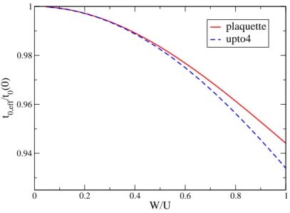
ing to the maximal extension considered in the calculation. In the two dimensional case
we have the nearest neighbor (NN) truncation, the plaquette calculation, which corre-
sponds to an extension of two and the double plaquette calculation, where terms with an
extension of three are considered. During the double plaquette calculation a vast amount
of terms is created so that we introduce another truncation scheme. In the upto4 trunca-
tion scheme we consider terms that fit on the double plaquette scheme but additionally
we require that these terms consist of at most four local operators. The number of local
operators contained in a term is denoted as its rank. This reduces the amount of terms
by a factor of 10.
4.4 Implementation 31
4.4. Implementation
With a higher maximal extension more and more terms fulfilling the truncation criteria are created.
As a result of the fast growing number of terms only the calculations belonging to the small truncation schemes like the minimal or the NN-truncation can be performed by hand. For higher truncation schemes the calculations are done by the use of a computer.
The program used in this thesis is implemented using the computer language C
++. The program is divided into two parts. The first part deals with the derivation of the dif- ferential equations for the coefficients. In the second part of the program these equations are solved numerically.
The program is based on the classes ’term’ and ’operator’, see Fig.4.6.
Fig. 4.6.: Schematic diagram for the 0n-generator
Operators are described by two numbers identifying the type of the operator. For each operator there are 16 possibilities as can be seen from the list 4.1. Beyond this the class operator contains a variable for the site on which the operator acts. The class term contains a vector of the type operator, which indicate the local operators, of which the term consists. Additionally the class contains the prefactor of the term. This prefactor is stored as an exact fraction to avoid numerical errors. For practical use this class contains two additional values. The first is the hash value of the term. Keeping this value speeds up the search for a certain term in the list of all terms. The second one is the multiplicity, which will be used in the context of symmetries as explained below.
The Hamiltonian itself is given as a vector of terms.
4.4.0.1. Setting up the differential equations
A structure chart of the first part of the program is shown in figure 4.7.
Fig. 4.7.: Structure chart for the used program
First of all the Hamiltonian is initialized. Then the program performs two loops in order to compute the comutator. One runs over all terms of the generator and one runs over all terms in the Hamiltonian. Here we make use of the fact that the generator consists of terms of the Hamiltonian itself. Therefore we just have to check if a certain term contributes to the generator and calculate the right prefactor.
The central part of the program is the calculation of the commutator. In this part we benefit from the representation of terms as products of local operators (see section 3.4).
The calculation of commutators of terms can thus be split into calculating commutators
of local operators. As there are bosonic as well as fermionic operators in the set of local
operators, we have to deal with commutators of two fermions, of two bosons and of a
fermion with a boson. Thus we have to express the commutators of terms by commutators
or anticommutators of its operators [Fis07]. In the case of two fermionic operators ˆ a
k, ˆ b
l,
4.4 Implementation 33
we obtain
hA, ˆ B ˆ
i=
n
Y
i=1
ˆ a
i,
m
Y
j=1
ˆ b
j
(4.4.1)
=
n
X
k=1 m
X
l=1
(−1)
(l−1)
k−1
Y
i=1
ˆ a
i!
l−1
Y
j=1
ˆ b
j
n
ˆ a
k, ˆ b
lo Ym
r=l+1
ˆ b
r! n Y
s=k+1
ˆ a
s!
(4.4.2) with m even. In this formula
{,}stands for the anticommutator of two operators.
The case of two bosonic operators ˆ a
kand ˆ b
las well as the case with one bosonic and one fermionic operator are covered by
h
A, ˆ B ˆ
i=
n
Y
i=1
ˆ a
i,
m
Y
j=1
ˆ b
j
(4.4.3)
=
n
X
k=1 m
X
l=1
k−1
Y
i=1
ˆ a
i!
l−1
Y
j=1
ˆ b
j
[ˆ a
k, ˆ b
j]
m
Y
r=l+1
ˆ b
r! n Y
s=k+1
ˆ a
s!