Competition of magnetic and superconducting ordering in one{dimensional generalized
Hubbard models
I n a u g u r a l - D i s s e r t a t i o n zur
Erlangung des Doktorgrades
der Mathematisch-Naturwissenschaftlichen Fakultat der Universitat zu Koln
vorgelegt von Christian Dziurzik aus Dramatal (Polen)
Koln 2003
Berichterstatter
Prof. Dr. J. Zittartz
Priv.-Doz. Dr. A. Schadschneider Prof. Dr. E. Muller-Hartmann Tag der mundlichen Prufung
11.02.2004
Contents
Preface 5
1. Interacting electrons in 1D 8
1.1. Fermi liquid theory and its breakdown . . . . 8
1.2. The concept of Tomonaga-Luttinger liquid . . . . 9
1.2.1. Free electrons in continuum limit . . . . 10
1.2.2. Scattering processes . . . . 11
1.2.3. Bosonic representation of the TL model . . . . 13
1.2.4. Single- and two-particle correlation functions . . . . 14
1.3. The Luther-Emery phase . . . . 15
1.4. Determination of K— andv— . . . . 18
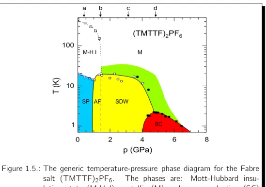
1.5. Quasi-1D organic (super-) conductors . . . . 19
2. The generalized Hubbard model 22 2.1. Derivation of the generalized Hubbard model . . . . 22
2.2. Some rigorous results for any lattice dimension . . . . 25
2.3. The Hubbard model in 1D . . . . 26
2.3.1. Symmetries and limiting cases . . . . 26
2.3.2. Exact solution: The Bethe ansatz . . . . 27
2.4. Superconductivity in extended Hubbard models . . . . 33
2.4.1. The extended Hubbard model . . . . 34
2.4.2. The Hirsch model . . . . 35
2.4.3. Thet`J model . . . . 36
3. The density matrix renormalization group technique 38 3.1. Exact diagonalization: The Lanczos method . . . . 39
3.1.1. Invariant subspace . . . . 39
3.1.2. The algorithm . . . . 39
3.1.3. Numerical implementation . . . . 40
3.2. Density matrix renormalization group (DMRG) . . . . 41
3.2.1. Numerical renormalization group (NRG) . . . . 42
3.2.2. Density matrix projection . . . . 43
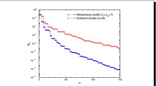
3.2.3. Truncation error & eigenvalue convergence . . . . 45
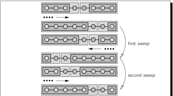
3.2.4. DMRG algorithms . . . . 46
3.2.5. Algorithm improvements . . . . 49
3.2.6. Correlation functions . . . . 53
3.2.7. DMRG and the matrix product ansatz (MPA) . . . . 54
3.2.8. Extensions of the DMRG technique . . . . 55
4. The Hubbard model with transverse spin exchange 59
4.1. Introduction . . . . 59
4.1.1. Analogy to the pair-hopping model . . . . 60
4.2. Weak-coupling results for the half-˛lled band . . . . 61
4.2.1. Bosonized Hamiltonian . . . . 61
4.2.2. Order parameters . . . . 63
4.2.3. The weak-coupling phase diagram . . . . 65
4.3. Numerical results at half-˛lling andU = 0 . . . . 67
4.3.1. Ground state energy . . . . 67
4.3.2. Excitation spectrum . . . . 68
4.3.3. Correlation functions . . . . 69
4.4. Numerical results at half-˛lling andU 6= 0 . . . . 73
4.4.1. Excitation spectrum . . . . 73
4.4.2. Correlation functions . . . . 73
4.5. Physical properties at quarter-˛lling . . . . 76
4.5.1. Excitation spectrum atU = 0 . . . . 76
4.5.2. Correlation functions . . . . 76
4.5.3. Excitation spectrum atU =t . . . . 79
5. Conclusion and Outlook 80 A. Implementation of the fermion sign in the DMRG method 82 B. Noninteracting fermions 84 B.1. Ground-State energy . . . . 84
B.2. Two-point correlations functions . . . . 85
Bibliography 88 Danksagungen 95 Anhange gem. Promotionsordnung 97 English Abstract . . . . 97
Deutsche Kurzzusammenfassung . . . . 99
Erklarung . . . 101
Lebenslauf . . . 103
Preface
The quest to understand the physics of strongly correlated fermion systems be- longs to the most challenging and active ˛elds in condensed matter physics. Vari- ous experiments on high-temperature superconductors (HTSC), heavy-fermion alloys and organic materials with their often reduced dimensionality have shown that strong interactions are a central ingredient for the understanding of their physical properties.
The aim of condensed matter theory is to understand the macroscopic beha- viour of ‰1023 interacting fermion systems, starting from a detailed microsopic description of the individual particles and the way they interact. However, the description is restricted to the theoretical models that capture all the necessary ingredients to discuss the physical behaviour one seeks to understand.
Historically, the theoretical basis for understanding the behaviour of electrons in solids is based on Landau’s Fermi-liquid theory in which the electrons are ex- pressed in terms of quasi-particles, describing single particle excitations of the non-interacting system, and in addition in terms of collective excitations. How- ever, in some new metallic systems, such as the HTSC, several anomalous prop- erties have been observed indicating that the Fermi-liquid theory does not provide a suitable description. Apart from the HTSC, this general picture of interact- ing quasi-particles is known to break down in one-dimensional metallic systems in which the concept of a Tomonaga-Luttinger liquid with purely collective excita- tions obeying Bose rather than Fermi statistics is successfully applied.
Numerous (lattice) models have been developed and studied in order to explain these various manifestations of strongly correlated electron behaviour. The most prominent one is theHubbard model, where the motion of electrons is controlled by the hopping amplitudet, in competition with the on-site Coulomb interaction U. The discovery of the HTSC compounds in 1986 has revitalized the investigation of the Hubbard model, since several mechanisms proposed to explain the HTSC invoke properties of the two-dimensional Hubbard model and probably also some one-dimensional aspects are relevant.
Despite of its simplicity only a few rigorous results exist (in any dimension). Hence it is very constructive to consider the one-dimensional counterpart, because ana- lytical as well as numerical tools are much more elaborated in one dimension.
Moreover, quantum ‚uctuations and collective e¸ects are generically strong in low dimensional systems providing a fascinating and challenging area for theoret- ical physicists.
A great variety of non-perturbative analytical and numerical techniques for low dimensional correlated systems have been developed, having their strengths and limitations. For instance, the one-dimensional Hubbard model can be solved ex-
actly by theBethe ansatz, but more realistic models including further interactions are no longer integrable. Other techniques like bosonization give a reliable de- scription of the physics only in the weak-coupling limit. However, in combination with (exact) numerical tools bosonization becomes a powerful technique.
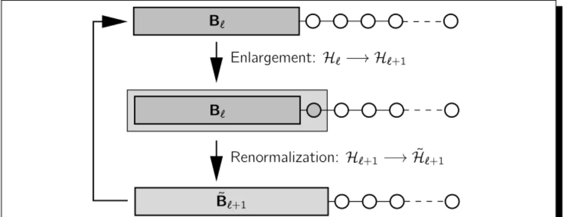
Due to the rapid evolution of computer technology, a considerable progress in the development of new numerical algorithms has been made. Perhaps the most important one is thedensity matrix renormalization group(DMRG) method which was developed by White in 1992. This numerical technique, which is the main tool of the present thesis, leads to highly accurate results for the low-energy physics of one-dimensional quantum systems. The DMRG algorihm is based on the following simple but e¸ective concept: the ground-state wavefunction as well as the low energy excitations of a large interacting chain are obtained by increasing the lattice size iteratively, starting with a small one that can be diagonalized exactly. The exponentially growing Hilbert space is controlled by a renormalization procedure in which ’less important’ degrees of freedom are integrated out.
Motivated by the discovery of triplet superconductivity (TS) inSr2RuO4 as well as the coexistence of the TS phase with ferromagnetism in UGe2, URhGe and Zr Zn2 and the indication that the quasi-one-dimensional conductors (Bechgaard salts) (T MT SF)2Cl O4 and (T MT SF)2P F6 under pressure are triplet supercon- ductors we study a rather simple extension of the Hubbard model with transverse (XY-type) anisotropy showing close proximity of triplet superconducting and fer- romagnetically ordered phases.
Layout of the Thesis
Chapter 1starts with an overview of interacting electrons in one dimension based on the concept of a Tomonaga-Luttinger (TL) liquid which is described in the framework of a weak-coupling continuum limit approach. The TL and Luther- Emery (LE) theory of an interacting gas model is used for the interpretation of our numerical results.
Chapter 2 is dedicated to the Hubbard model and its extensions. Starting with the derivation of Hubbard’stight-bindingapproximation of electrons in a Coulomb potential, we summarize basic properties of these lattice models. In one dimension, where the (extended) Hubbard model belongs to the universality class of either a TL liquid or a LE phase, the pure Hubbard model is exactly solvable by the Bethe ansatz. We give an outline of this technique and close with a discussion of some extended versions of the Hubbard model exhibiting ’superconducting’
phases, characterized by dominant pair correlations.
Chapter 3 gives a detailed description of White’s density matrix renormalization group method and its historical context, beginning with the Lanczos algorithm which is applied within our DMRG routine. After outlining the two types of al- gorithms and its improvements, we show how to evaluate (fermionic) local expect- ation values and correlation functions. Finally, the relation to the matrix product ansatz and some extensions of the DMRG method will be disccused.
Chapter 4 presents our numerical results for the Hubbard model with transverse spin-exchange. At ˛rst, we re‚ect the weak-coupling phase diagram using the
Contents 7 bosonization technique and continue with the analysis of our numerical data for the half-˛lled case con˛rming the bosonization results. Additionally, we discuss a new phase, which is absent in the weak-coupling investigation, and close this part with a discussion of the phase diagram for the half-˛lled model. Afterwards, DMRG data for the quarter-˛lled band are analyzed, as a basis for further studies.
Chapter 5contains the conclusion of this thesis and gives perspectives for further research on the presented topic.
Why are solids in one dimension so special? Already the topology of the Fermi surface which is described by only two discrete points in one dimension and a continuous sphere in more than one dimension indicates that one dimensional interacting systems might behave di¸erent. In two and three dimensions the low-energy physics of interacting fermions is well described by the Fermi liquid theory developed by Landau [1, 2, 3]. However, in one dimension Landau’s theory breaks down and the unusual physical behaviour is characterized by the so-called Tomonaga-Luttinger liquid, a name coined by Haldane [4]. The basic model in this context is usually called Tomonaga-Luttinger model [5, 6] and was solved exactly by applying thebosonization method [7].
After outlining the collapse of Fermi liquid theory in 1D, the description of the Luttinger liquid as a universality class of gapless one dimensional interacting sys- tems will be the subject of the following sections. In addition, a universality class characterized by a gap in the spin excitation spectrum will be discussed. The corresponding model is called Luther-Emery model [8].
1.1. Fermi liquid theory and its breakdown
In Landau’s theory the fundamental degrees of freedom of the system are quasi- particles which allow a one-to-one correspondence between non-interacting and weakly interacting systems. This is possible because weak interaction in principle does not destroy the Fermi surface, i.e. the shape of the momentum distribution function nff(k) changes, but the ˛nite discontinuity at the Fermi surface jkj=kF remains (cf. with the left-hand side of Fig. 1.1).
This discontinuity can be explained on the microscopic level in terms of Green’s functions. In the non-interacting case the one-particle Green’s function
G0(k; !) = 1
!+ i‹`"0(k) (1.1) has a pole on the real axis describing a single-particle excitation with a well de˛ned dispersion ! ="0(k). Note that the corresponding spectral function is simply a delta-function, i.e. A0(k; !) =‹(!`"0(k)). However, if interactions are switched on, then the Green’s function has the modi˛ed form
G(k; !) = 1
!+ i‹`"0(k)`˚(k; !); (1.2) where the di¸erence between the non-interacting and interacting Green’s functions is expressed through the self-energy ˚(k; !) which contains all many-body e¸ects.
1.2 The concept of Tomonaga-Luttinger liquid 9 Now the single-particle excitations are given by the poles of G(k; !) while the self-energy ˚(k; !) provides the damping of these excitations. However, a single solution which is characterized by only one pole with ˛nite residue
zk`1= 1` @˚
@!
!=0;k=kF »1; (1.3)
implies a normal Fermi liquid. The amplitude zk gives the magnitude of the discontinuity of the momentum distribution function at the Fermi surface (cf.
with the left-hand side of Fig. 1.1). The corresponding Green’s function becomes G(k; !) =Gincoh(k; !) + zk
!`"(k) + i=fik; (1.4) after expanding the self-energy to second order around the Fermi surface. Of course, it is essential that ˚(k; !) has an analytic expansion about ! = 0 and jkj=kF. For long timescales
fik`1=`zkIm ˚(k; != 0)!0 (k !kF) (1.5) the second term of Eq. (1.4) gives a broadened delta-peak in the spectral func- tion, whereas Gincoh(k; !) corresponds to a smoothincoherent background. The damped peak at the energy "(k) / "0(k)zk expresses the fact that excitations have the character of quasi-particles. The breakdown of the Fermi liquid theory in
FL TLL
1 nff(k)
kF k
1 nff(k)
k kF
zk
Figure 1.1.: The ˛gure shows a qualitative plot of the single-particle mo- mentum distribution functionnff(k) at temperatureT = 0. Left:
˛nite discontinuity at the Fermi momentum kF for a system of interacting fermions in more than one dimension (FL: Fermi li- quid). Right: absence of a discontinuity in an interacting system in one dimension (TLL: Tomonaga-Luttinger liquid). The dashed lines show the non-interacting case.
1D is signalled by either the appearance of multiple solutions indicated by multiple poles or ifzk = 0, manifesting a continuous momentum distribution function, as illustrated in the right-hand side of Fig. 1.1.
1.2. The concept of Tomonaga-Luttinger liquid
In the limit of weakly interacting fermions only states close to the two Fermi points˚kF are important. For this reason it is possible to linearize the spectrum
"(k) around ˚kF which is leading to two branches of particles, the right movers and theleft movers. Note that in a simple lattice model (see Sec. 2.1 for details) one would have "(k) = `2tcos(k), where t describes the motion of particles to neighbouring lattice sites. In the continuum-limit theory one then obtains four scattering processes which describe the interaction among these particles.
Two scattering processes characterize the Tomonaga-Luttinger (TL) model which can be solved exactly within the framework of the bosonization technique. The determined TL parameters describe the physics of this model. This will be the subject of the following parts.
1.2.1. Free electrons in continuum limit
The microscopic Hamiltonian describing non-interacting electrons has the well- known form
H0=X
k;ff
"(k)ck;ffy ck;ff; (1.6)
where ck;ff and ck;ffy are the standard annihilation and creation operators for an electron with momentumk and spinff=f";#g, expressed in second quantization.
The summation over k is limited to the ˛rst Brillouin zone [`ı=a0; ı=a0], where a0 is the lattice spacing. Note that each momentum state k can be ˛lled by two electrons of opposite spins (Pauli principle), thus k = 2ı=Lˆn with n = 0;˚1;˚2: : : ;˚(L=2`1); L=2 has to be used (here witha0= 1). The quantity L is the total number of lattice sites.
In the continuum limit (a0 !0) the Brillouin zone extends to [`1;1] and the annihilation and creation operators are mapped to analogous fermionic ˛elds. For instance, the ˛eld operator of the corresponding annihilation operatorck;ff and its inverse transformation are given by
ff(x) = 1 pL
+1
X
k=`1
eikxck;ff and ck;ff = 1 pL
Z +L=2
`L=2
d x e`ikx ff(x); (1.7)
where the momentumk = 2ı=Lˆn is not bounded, i.e. n= 0;˚1;˚2: : :. The continuous variable x is related to the discrete lattice site n throughx !na0. In the weak-coupling approach one assumes that the low energy physics is only relevant near the two Fermi points ˚kF. Therefore, it is possible to linearize the energy spectrum"(k) =vF(k`kF) for right movers and"(k) =`vF(k+kF) for left movers with
vF = @"(k)
@k
k=kF / @cos(k)
@k
k=kF
; (1.8)
which expresses the relation between the linearized spectrum and the lattice one.
Moreover, one decomposes the sum in expression (1.7) into two parts, corres- ponding to k > 0 and k < 0, and then shifts each sum by ˚kF so that k = 0
1.2 The concept of Tomonaga-Luttinger liquid 11
corresponds to the Fermi points:
ff(x) = 1 pL
X
k>0
eikxck;ff+ 1 pL
X
k<0
eikxck;ff
= 1
pL
+1
X
k=`kF
ei(k+kF)xck+k
F;ff+ 1 pL
+kF
X
k=`1
ei(k`kF)xck`k
F;ff
” eikFx R;ff(x) +e`ikFx L;ff(x) (1.9) The smooth ˛eld operators R and L describe right- and left-movers with mean momenta centered around˚kF. By using formula (1.9) the real space counterpart of the free fermion Hamiltonian (1.6) then reads
H0=`ivF
Z +L=2
`L=2
d xX
ff
y
R;ff(x)@x R;ff(x)` L;ffy (x)@x L;ff(x)
: (1.10) For the derivation one must note the following: the cross terms between left and right components will make no contribution because the smooth left and right
˛elds have no overlap if the ‚uctuations around ˚kF are assumed to be small.
Finally, a ˛rst order Taylor expansion has been applied
”;ff(x+a0)ı ”;ff(x) +a0@x ”;ff(x) (1.11) for each branch ” 2 fR; Lg of the dispersion curve. Sometimes we will use the notation”2 f+1;`1ginstead ofRandLand furthermoreff2 f+1;`1ginstead of"and #.
1.2.2. Scattering processes
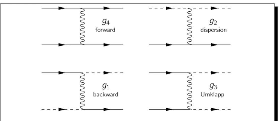
Due to the special topology of the one-dimensional Fermi surface, the space for collisions between particles is strongly limited compared to higher dimensional systems. By energy and momentum conservation alone, the corresponding low- energy scattering processes, restricted to the two Fermi points˚kF, can be clas- si˛ed into four di¸erent types. These four species of collisions are illustrated in Fig. 1.2. Next, the coupling constants for electrons with parallel spins will be denoted by the subscript ’k’ and those with anti-parallel spins by ’?’. Following [9], the scattering process with coupling g4 describes forward scattering, where all four participating electrons belong to a single branch. Using the smooth ˛eld operators R and L the Hamiltonian reads
Hgint4 /X
ff;ff0
1
2 g4k‹ff;ff0+g4?‹ff;`ff0 X
”
”;ffy y
”;ff0 ”;ff0 ”;ff: (1.12) The dispersion, characterized by g2, corresponds to similar events but involves electrons on both branches. The interacting Hamiltonian has the form
Hintg2 /X
ff;ff0
g2k‹ff;ff0+g2?‹ff;`ff0 y
R;ff y
L;ff0 L;ff0 R;ff: (1.13)
backward
g1 g3
g2
g4
forward dispersion
Umklapp
Figure 1.2.: The four scattering processes in the so-called g-ology nomen- clature for right-moving (solid lines) and left-moving (dashed lines) electrons in one dimension. In all these processes the spin dependence is suppressed.
Note that in both processes the associated momentum transfer is small. The g1event describes backward scattering, where each electron changes branch but keeps its spin. This contribution is given by
Hgint1 /X
ff;ff0
g1k‹ff;ff0+g1?‹ff;`ff0 y
R;ff y
L;ff0 R;ff0 L;ff: (1.14) The momentum transfer is of order 2kF. Finally, the Umklapp process (two left electrons become right electrons or vice-versa) is denoted byg3 and is important only if the band is half-˛lled, i.e. only if 4kF is equal to a reciprocal lattice vector.
The process is expressed by the term Hgint3 /X
ff;ff0
1
2 g3k‹ff;ff0+g3?‹ff;`ff0 X
”
”;ffy y
”;ff0 `”;ff0 `”;ff: (1.15) Since the e¸ect of g1k is indistinguishable from that ofg2k, one may set g1k = 0 without loss of generality. A spin-rotationally invariant model further reduces the number of independent couplings. Note that scattering processes of typeg2 and g4do not break symmetries. In contrast, the Umklapp processg3breaks the con- servation of individual charge currents and a charge gap opens if the interactions are attractive (g3 < 0). Similarly, the attractive backscattering process g1 < 0 breaks the conservation of individual spin currents and a gap in the spin excitation spectrum opens.
A detailed renormalization group analysis of this interacting gas model is given by S«olyom [9]. For particular combinations of these coupling constants exact solutions are known. On the one hand there is the gapless Tomonaga-Luttinger (TL) model and on the other hand there is the Luther-Emery (LE) model having a gap in the spin excitation spectrum. Both models can be solved exactly by expressing the fermionic ˛eld operators in terms of boson operators [7, 8].
1.2 The concept of Tomonaga-Luttinger liquid 13 1.2.3. Bosonic representation of the TL model
The TL model is a particular model of the interacting Fermi gas, Eqs. (1.12)- (1.15) and Eq. (1.10), in which the bosonization technique yields an exact solu- tion. The Hamiltonian of the TL model for spin-1=2 particles reads
HTL = H0+Hgint2 +Hgint4 (1.16)
= `ivF Z
d xX
ff;”
” ”;ffy (x)@x ”;ff(x) +
Z
d xX
ff;ff0
g2k‹ff;ff0+g2?‹ff;`ff0 y
R;ff(x) yL;ff0(x) L;ff0(x) R;ff(x) +
Z d x 2
X
ff;ff0;”
g4k‹ff;ff0+g4?‹ff;`ff0 y
”;ff(x) y”;ff0(x) ”;ff0(x) ”;ff(x): A bosonic formulation of (1.16) is described by two independent bosonic ˛elds, one representing the charge and the other the spin degrees of freedom. The fermionic ˛eld operators ”;ff are represented by bosonic operators ˘”;ff via the identity [10]
”;ff(x) = 1
p2ı¸F”;ffexp [i˘”;ff(x)] ; (1.17) where¸is a short distance cut-o¸ that is taken to zero at the end of the calcula- tion and the so-calledKlein factors F”;ffare responsible for reproducing the correct anticommutation relations between di¸erent fermionic species. The bosonic ˛elds
˘”;ff, which obey
˘”;ff(x);˘y”0;ff0(x0)
=`iı ‹”;”0‹ff;ff0sign(x`x0); (1.18) in turn are combinations of bosonic ˛eldsffi— and their conjugate momenta @x„—, where the subscript denotes charge (—=c) or spin (—=s) degrees of freedom.
The relation is given by
˘”;ff = rı
2[(„c`”ffic) +ff(„s`”ffis)] ; (1.19) where ffi— and„— satisfy the following commutation relation
ffi—(x); „—0(x0)
= i
2‹—;—0sign(x`x0): (1.20) From a physical point of view, ffic and ffis are the phases of the charge density wave (CDW) and spin density wave (SDW) ‚uctuations, i.e.
(x)ı r2
ı@xffic(x) and Sz(x)ı r 1
2ı@xffis(x); (1.21) whereas„c describes the superconducting phase (see chapter 4 for details). The Hamiltonian can now be expressed as a sum of two decoupled pieces of bosonic oscillators involving either charge or spin density wave eigenmodes
HBTL = Z
d x X
—=c;s
v—K—
2 [@x„—(x)]2+ v—
2K—[@xffi—(x)]2
: (1.22)
In terms of the parameters gic ” gik +gi? and gis ” gik `gi? (i = 2;4) the charge and spin velocities are
v—=vF s
1 + g4—
2ıvF 2
` g2—
2ıvF 2
: (1.23)
One spectacular consequence is the so-called spin-charge separation (cf. with Eq. (1.22)) which is completely absent in higher dimensions. In this description this is due to the fact that spin and charge density modes propagate with di¸erent velocities (vs 6= vc) and therefore will separate with time. The parameters K—, which determine the decay behaviour of the correlation functions, are
K—=
s2ıvF +g4—`g2—
2ıvF +g4—+g2— : (1.24)
Note that the properties of the TL model are completely described by the set of parameters fv—; K—g.
1.2.4. Single- and two-particle correlation functions
In this section we give a summary of the correlation functions from which the phys- ical properties of the TL model may be obtained. Here we will restrict ourselves to the SU(2) spin-invariant model withKs = 1.
From our previous discussion of spin-charge separation it is already obvious that the TL system isnot a Fermi liquid. This can be made more precise. After apply- ing the Fourier transformation on the single-particle Green’s functionGff(x ; t) the corresponding momentum distribution function in the vicinity of the Fermi surface reads
nff(k)ınff(kF)`const.ˆsign(k`kF)jk`kFj‚; (1.25) where the exponent ‚ has the explicit form
‚ = 1
4 Kc+Kc`1`2
–0: (1.26)
Note that for any nonvanishing interaction (Kc 6= 1) the discontinuity at kF is absent, i.e. nff(k) is continuous (cf. with section 1.1).
The coe‹cientKc also determines the long-distance decay behaviour of all other correlation functions hOy(x)O(x0)i in which the order parameter O describes an instability of the systems. The relevant operators which can take on non-zero expectation values are the 2kF CDW and SDW instabilities and the singlet (SS) and triplet (TS) superconducting operators. An explicit fermionic and bosonic expression will be discussed in chapter 4.
The asymptotic shape of the correspondig correlation functions can be calculated exactly (see [11] and references therein). In detail, one obtains
1. for the density-density correlation (similar to CDW) (0)(r)
‰ A0
r2 +A1cos(2kFr)
r1+Kc +A2cos(4kFr)
r4Kc +: : : ; (1.27)
1.3 The Luther-Emery phase 15 2. for the spin-spin correlation (similar to SDW)
Sz(0)Sz(r)
‰ B0
r2 +B1cos(2kFr)
r1+Kc +: : : ; (1.28) 3. for the singlet-pair correlation
OySS(0)OSS(r)
‰ C0
r1+Kc`1 +C1cos(2kFr)
rKc+K`1c +: : : (1.29) 4. and for the triplet-pair correlation
OyTS(0)OTS(r)
‰ D0
r1+Kc`1 +D1cos(2kFr)
rKc+Kc`1+2 +: : : : (1.30) The constant coe‹cients Ai; Bi; Ci andDi are model dependent. The algebraic decay of each correlation function is characterized by the exponentKc only. For Kc < 1 spin or charge density ‚uctuations will be enhanced, while for Kc > 1 pairing ‚uctuations will dominate.
Note that logarithmic corrections, sometimes included in the above formulae [12], have not been taken into account because they are not important as long as one is only interested in the asymptotics r fl1 of the correlations.
In general, 1D quantum-systems with short-range interaction and gapless excita- tions are critical at zero temperature. In such a case, various correlation functions showpower-lawdecay. Otherwise, i.e. in the presence of a gap (cf. with Sec. 1.3), they may decay exponentially and the corresponding correlation length ‰ is de- termined by the gap. Closing of a gap indicates a divergent correlation length.
In the limit ‰ ! 1 the corresponding correlations show power-law decay. Note that long-range order (LRO) in 1D quantum-systems at ˛nite temperatureT >0 is forbidden by the Mermin-Wagner theorem [13]. This statement is also valid for T = 0 [14] as long as the models are described by continuous symmetries.
However, models with a discrete symmetry (cf. with chapter 4) admit LRO even in 1D. Therefore, 1D phases are best characterized by the asymptotic behaviour of the correlation functions.
1.3. The Luther-Emery phase
The TL model is very restrictive since the interaction parameters g2 and g4 are associated with a small momentum transfer whereas any realistic model with interaction of type
Hint = 1 L
X
k;k0;q;ff;ff0
V(q)ck+q;ffy cky0`q;ff0ck0;ff0ck;ff (1.31) also contains contributions with q – 2kF. Note that the choice of parameters under which the numbers of right and left movers are conserved is essential in guaranteeing the exact solvability of this model.
Additional terms like g1 or g3 destroy the symmetry because they change the individual particle numbers. The Hamiltonian of the TL model (1.22) in which processes like
HBg1? = g1? 2(ı¸)2
Z
d xcos(p
8ıffis) or (1.32) HBg3? = g3?
2(ı¸)2 Z
d xcos(p
8ıffic) (1.33)
are included is, in general, no longer exactly solvable but a renormalization group (RG) analysis permits important insights about the in‚uence of such terms.
For simplicity, let us focus on a spin-independent Hamiltonian (1.12){(1.14) with gik = gi? = gi (i = 1;2;4) which can be realized in a SU(2) symmetric model.
The RG ‚ow equations for cut-o¸ dependent interactions gi(‘) are quite simple [9] and translate into
d
d ‘g1(‘) = ` 1
ıvFg12(‘) and (1.34) d
d ‘g2(‘) = ` 1
2ıvFg21(‘): (1.35)
after short-distance degrees of freedom have been integrated out. Note that g4
is not renormalized and thatg1(‘) can be determined from the ˛rst equation only g1(‘) = g1
1 +‘ıvg1
F
(1.36) where g1 is the starting value. Furthermore, it is easy to see that
g1(‘)`2g2(‘) =g1`2g2 (1.37) holds by subtracting twice the second equation from the ˛rst in Eq. (1.34). There are two di¸erent types of ‚ow:
➊ For g1 –0 one renormalizes to the ˛xed line g1˜ = 0 andg2˜ =g2`g1=2, where the notationgi˜”gi(‘! 1) was used. The˛xed point Hamiltonian is a TL model with repulsive interactions in which the g1-interaction is irrelevant.
➋ For g1 < 0 the solution (1.36) shows that g1(‘) diverges at a ˛nite value of ‘, i.e. long before reaching this point the perturbational analysis breaks down. However, one should notice that, well before the divergence, one has left the weak-coupling regime where Eq. (1.34) and (1.35) are valid.
Therefore, one should not overinterpret the divergence and just remember that the RG scales to strong coupling.
When g1k = g1? < 0, the system is described by the presence of a ˛nite spin gap ´s. Further RG investigations show that the gap remains for all g1?<0 and jg1?j > g1k. For the anisotropic case, Luther and Emery have shown that for the
1.3 The Luther-Emery phase 17 particular point Ks = 1=2 the model is exactly solvable. At this point a new set of spinless fermions can be de˛ned
¯”” 1
p2ı¸F”exp[ip
ı=2(„s `2”ffis)] (1.38) and the spin part of the correspondingrefermionized Hamiltonian then reads
Hs =`ivsX
”
”¯y”@x¯”+ ´s(¯yR¯L+ h.c.): (1.39) This Hamiltonian is easy to diagonalize and the exact result indicates an energy spectrum
Es = q
vs2k2+ ´2s with a ˛nite gap ´s ‰ jg1?j
2ı¸ : (1.40)
This gap has drastic consequences for the physical properties, i.e. correlations such as SDW and triplet pairing are not critical and decay exponentially with correlation length ‰s = vs=´s, whereas CDW and SS correlators are enhanced compared to the case with no spin gap.
(SS) TS SDW
(CDW)
SS (CDW)
SS (SS)
CDW CDW
Kc
g1?
2 1
1/2
Figure 1.3.: Phase diagram in theg1?-Kc plane for a 1D interacting gas model in the absence of Umklapp scattering (from [15]). Correlations indicated in parentheses have the same exponents as the dom- inant ones but are logarithmically weaker. At g1? – 0 the sys- tem belongs to the TL liquid with gapless excitations, whereas the shaded region (g1? < 0) contains the spin gapped phases.
Here, ‚uctuations appearing in parentheses diverge with a smaller power-law exponent than the dominant ones.
Without logarithmic corrections their asymptotic form explicitly reads [8]
1. for the density-density correlation (0)(r)
‰ A0
r2 +A1cos(2kFr)
rKc +A2cos(4kFr)
r4Kc +: : : (1.41)
![Figure 1.4.: The critical exponent K c (here denoted by K ) for the repulsive Hubbard model as a function of the band ˛lling n = N=L with U=t = 1 for the top curve and with U=t = 2; 4; 8; 16 for the bottom curves (from [12]).](https://thumb-eu.123doks.com/thumbv2/1library_info/3707832.1506236/19.918.162.717.87.327/figure-critical-exponent-denoted-repulsive-hubbard-function-curves.webp)
![Figure 2.1.: A schematic illustration of the the tight-binding approximation (taken from [28])](https://thumb-eu.123doks.com/thumbv2/1library_info/3707832.1506236/23.918.160.712.297.675/figure-schematic-illustration-tight-binding-approximation-taken.webp)
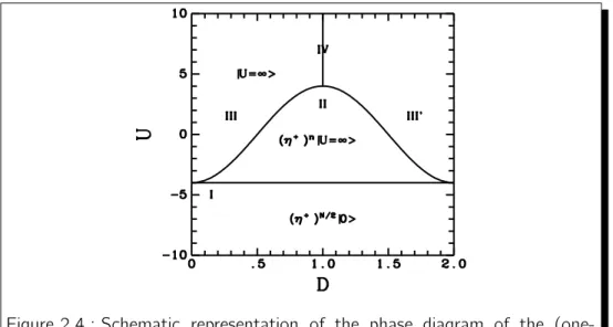
![Figure 2.5.: The phase diagram for the one-dimensional t ` J model (taken from Ref. [86])](https://thumb-eu.123doks.com/thumbv2/1library_info/3707832.1506236/37.918.160.720.88.350/figure-phase-diagram-dimensional-j-model-taken-ref.webp)