Deep Residual Learning and PDEs on Manifold
Zhen Li ∗ Zuoqiang Shi†
Abstract
In this paper, we formulate the deep residual network (ResNet) as a control problem of transport equation. In ResNet, the transport equation is solved along the character- istics. Based on this observation, deep neural network is closely related to the control problem of PDEs on manifold. We propose several models based on transport equa- tion, Hamilton-Jacobi equation and Fokker-Planck equation. The discretization of these PDEs on point cloud is also discussed.
keywords: Deep residual network; control problem; manifold learning; point cloud; trans- port equation; Hamilton-Jacobi equation
1 Deep Residual Network
Deep convolution neural networks have achieved great successes in image classification.
Recently, an approach of deep residual learning is proposed to tackle the degradation in the classical deep neural network [7, 8]. The deep residual network can be realized by adding shortcut connections in the classical CNN. A building block is shown in Fig. 1. Formally, a building block is defined as:
y=F(x,{Wi}) +x.
Here x and y are the input and output vectors of the layers. The function F(x,{Wi}) represents the residual mapping to be learned. In Fig. 1,F =W2·σ(W1·σ(x)) in which σ= ReLU◦BN denotes composition of ReLU and Batch-Normalization.
∗Department of Mathematics, Hong Kong University of Science & Technology, Hong Kong. Email:
mazli@ust.hk.
†Yau Mathematical Sciences Center, Tsinghua University, Beijing, China, 100084. Email:
zqshi@tsinghua.edu.cn.
arXiv:1708.05115v3 [cs.IT] 25 Jan 2018
BN xl
xl+1 ReLU Conv.
BN ReLU Conv.
+
Figure 1: Building block of residual learning [8].
2 Transport Equation and ResNet
Consider the the terminal value problem of linear transport equation in Rd:
∂u
∂t −v(x, t)· ∇u= 0, x∈Rd, t≥0, u(x,1) =f(x), x∈Rd.
(1)
where v(x, t) is a given velocity field, f is the composition of the output function and the fully connected layer. If we use the softmax activation function,
f(x) =softmax(WF C·x), (2)
whereWF C is the weight in the fully connected layer, softmax function is given by softmax(x)i = exp(xi)
P
jexp(xj).
which models posterior probability of the instance belonging to each class.
It is well-known that the solution at t = 0 can be approximately solved along the characteristics:
dx(t;x)
dt =v(x(t;x), t), x(0;x) =x. (3)
We know that along the characteristics, u is a constant:
u(x,0) =u(x(1;x), T) =f(x(1;x)).
Let {tk}Lk=0 with t0 = 0 and tL = 1 be a partition of [0,1]. The characteristic of the transport equation (3) can be solved by using simple forward Euler discretization from x0(x) =x:
Xk+1(x) =Xk(x) + ∆tv(Xk(x), tk), (4)
where ∆tis the time step. If we choose the velocity field such that
∆tv(x, t) =W(2)(t)·σ
W(1)(t)·σ(x)
, (5)
where W(1)(t) and W(2)(t) corresponds to the ’weight’ layers in the residual block, σ = ReLU◦BN, one step in the forward Euler discretization (4) actually recovers one layer in the deep ResNets, Fig. 1. Then the numerical solution of the transport equation (1) at t= 0 is given by
u(x,0) =f(XL(x)) (6)
This is exactly the output we get from the ResNets.
If x is a point from the training set, we already have a labeled valueg(x) on it. Then we want to match the output value given in (6) and g(x) to train the parameters in the velocity filed (5) and the terminal value.
Based on above analysis, we see that the training process of ResNet can be formulated as an control problem of a transport equation inRd.
∂u
∂t(x, t)−v(x, t)· ∇u(x, t) = 0, x∈Rd, t≥0, u(x,1) =f(x), x∈Rd, u(xi,0) =g(xi), xi∈T.
(7)
whereT denotes the training set. g(xi) is the labeled value at sample xi. Functionu may be scalar or vector value in different applications.
So far, we just formulate ResNet as a control problem of transport equation. This model will inspire us to get new models by replacing different component in the control problem.
3 Modified PDE model
From the PDE point of view, ResNet consists of five components:
• PDE: transport equation;
• Numerical method: characteristic+forward Euler;
• Velocity filed model: v(x, t) =W(2)(t)·σ W(1)(t)·σ(x)
;
• Terminal value: f(x) =softmax(WF C·x);
• Initial value: label on the training setg(xi), xi∈T.
In five components listed above, the last one, ”initial value”, is given by the data and we have no other choice. All other four components, we can consider to replace them by other options. Recently, there are many works in replacing forward Euler by other ODE solver. Forward Euler is the simplest ODE solver. By replacing it to other solver, we
may get different network. In some sense, in DenseNet [9], forward Euler is replaced by some multi-step scheme. There are many numerical schemes to solve the ODE (3). Some numerical scheme may be too complicated to be used in DNN. Constructing good ODE solver in DNN is an interesting problem worth to exploit in our future work.
3.1 Terminal Value
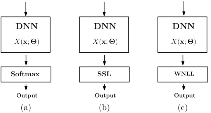
From the control problem point of view, the softmax output function is not a good choice for terminal vaule, since they are pre-determined, may be far from the real value. Semi- supevised learning (SSL) seems provides a good way to get terminal value instead of the pre-determined softmax function as shown in Fig. 2(b).
DNN
X(x;Θ)
Output Softmax
DNN
X(x;Θ)
Output SSL
DNN
X(x;Θ)
WNLL
Output
(a) (b) (c)
Figure 2: (a): standard DNN; (b): DNN with semi-supervised learning; (c): DNN with last layer replaced by WNLL.
Recently, we try to use weighted nonlocal Laplacian [11] to replace softmax and the results is pretty encouraging [12].
3.2 Velocity Field Model
In transport equation, we need to model a high dimensional velocity filed. In general, it is very difficult to compute a high dimensional vector field. In the application associated to images, the successes of CNN and ResNet have proved that the velocity filed model based on convolutional operators, (8), is effective and powerful.
v(x, t) =W(2)(t)·σ
W(1)(t)·σ(x)
. (8)
However, this is not the only way to model the velocity field. Moreover, for the applications in which convolutional operator makes no sense, we have to propose alternative velocity model. Here, we propose a model based on Hamilton-Jacobi equation to reduce the degree of freedom in the velocity field.
Notice that even though the velocity v(x, t) is a high dimensional vector field, in the tranport equation, only the component along ∇u is useful. Based on this observation, one
idea is only model the component along ∇u by introducing ¯v(x, t) = v(x, t)·n(x, t) and n(x, t) = |∇∇Mu
Mu|. Then the transport equation in (7) becomes a Hamilton-Jacobi equation.
We get a control problem of Hamilton-Jacobi equation.
∂u
∂t −¯v(x, t)· |∇u|= 0, x∈Rd, t≥0, u(x,0) =f(x), x∈ M, u(xi,1) =g(xi), xi ∈T.
(9)
In (7), the velocity field, v(x, t), is a d-dimensional vector field. Meanwhile, in the Hamilton-Jacobi model, we only need to model a scalar function ¯v(x, t). The number of parameters can be reduced tremendously. To model a scalar function is much easier than model a high dimensional vector field. There are already many ways to approximate ¯v(x, t).
1. The simplest way is to model ¯v(x, t) as a linear function with respect to x, i.e.
¯
v(x, t) =w(t)·x+b(t), w(t)∈Rd, b(t)∈R. (10) Although ¯v(x, t) is a linear function to x, the whole model (9) is not a linear model since Hamilton-Jacobi equation is a nonlinear equation.
2. Neural network is consider to be an effective way to approximate scalar function in high dimensioanl space. One option is a simple MLP with one hidden layer as shown in Fig. 3.
Weight
d×m ReLU
Weight m×1
x∈Rd ¯v(x)∈R
Figure 3: MLP model with one hidden layer for ¯v(x, t) in (9).
There are many other neural networks in the literature to approximate scalar function in high dimensioanl space.
3. Radial basis function is another way to approximate ¯v(x, t). Radial functions centered at each sample point are used as basis function to approximate ¯v(x, t), i.e.
¯
v(x, t) = X
xj∈P
cj(t)R |x−xj|2 σj2
!
(11) wherecj(t), j= 1,· · ·,|P|are coefficients of the basis function. One often used basis function is Gaussian function,R(r) = exp(−r).
Another difficulty in solving model (9) is efficient numerical solver of Hamilton-Jacobi equation in high dimensional space. Hamilton-Jacobi equation is a nonlinear equation which is more difficult to solve than linear transport equation in (7). Recently, fast solver of Hamilton-Jacobi equation in high dimensional space attracts lots of attentions and many efficient methods have been developed [1, 2, 3, 4, 5, 6].
3.3 PDEs on point cloud
Another thing we can consider to change is the characteristic method in solving the transport equation. There are many other numerical method for transport equation based on Eulerian grid. However, in these methods, we need to discretize the whole spaceRdby Eulerian grid, which is impossible whendis high. So in high dimensional spaceRd, characteristic method seems to be the only practical numerical method to solve the transport equation. On the other hand, we only need to solve the transport equation in the dataset instead of the whole Rd space. Usually, we can assume that the data set sample a low dimensional manifold M ⊂Rd, then the PDE can be confined on this manifold. The manifold is sampled by the point cloud consists of the data set including the training set and the test set. Then the numerical methods in point cloud can be used to solve the PDE.
Transport equation In the manifold, the transport equation model (7) can be rewritten as follows:
∂u
∂t −v(x, t)· ∇Mu= 0, x∈ M ⊂Rd, t≥0, u(x,0) =f(x), x∈ M,
u(xi,1) =g(xi), xi ∈T.
(12)
∇M denotes the gradient on manifold M. Let X : V ⊂ Rm → M ⊂ Rd be a local parametrization of Mand θ∈ V. For any differentiable function u :M →R, let U(θ) = f(X(θ)), define
Dku(X(θ)) =
m
X
i,j=1
gij(θ)∂Xk
∂θi (θ)∂U
∂θj(θ), k= 1,· · ·, d. (13) where (gij)i,j=1,···,m = G−1 and G(θ) = (gij)i,j=1,···,m is the first fundamental form which is defined by
gij(θ) =
d
X
k=1
∂Xk
∂θi (θ)∂Xk
∂θj (θ), i, j= 1,· · · , m. (14)
∇M is defined as
∇Mu= (D1u, D2u,· · · , Ddu). (15) In (12), the manifold Mis sampled by the data setP andP is a collection of unstruc- tured high dimensional points. Unlike the classical numerical methods which solve PDE on regular grids (or meshes), in this case, we need to discretize PDE on unstructured high di- mensional point cloud P. To handle this kind of problems, recently, point integral method (PIM) was developed to solve PDE on point cloud. In PIM, gradient on point cloud is approximate by an integral formula [10].
Dku(x) = 1 wδ(x)
Z
M
(u(x)−u(y)) (xk−yk)Rδ(x,y)dy. (16)
wherewδ(x) =R
MRδ(x,y)dy,
Rδ(x,y) =R
kx−yk2 δ2
. (17)
The kernel functionR(r) :R+→R+is assumed to be aC2 function with compact support.
Corresponding discretization is Dku(x) = 1
¯ wδ(x)
X
y∈P
(u(x)−u(y)) (xk−yk)Rδ(x,y)V(y). (18)
¯
wδ(x) =P
y∈PRδ(x,y)V(y) and V(y) is the volume weight ofy depends on the distribu- tion of the point cloud in the manifold.
Hamilton-Jacobi equation We can also confine the Hamilton-Jacobi equation in (9) in the manifold.
∂u
∂t −v(x, t)¯ · |∇Mu|= 0, x∈ M ⊂Rd, t≥0, u(x,0) =f(x), x∈ M,
u(xi,1) =g(xi), xi ∈T.
(19)
On the point cloud, one possible choice to discretize |∇Mu|is
|∇Mu(x)|= Z
M
w(x,y)(u(x)−u(y))2dy 1/2
. (20)
¯
v(x, t) can be modeled in the way discussed in the previous section.
PDEs with dissipation We can also consider to add dissipation to stabilize the PDEs.
∂u
∂t −¯v(x, t)· |∇Mu|= ∆Mu, x∈ M ⊂Rd, t≥0, u(x,0) =f(x), x∈ M,
u(xi, t) =g(xi), xi ∈S, u(xi,1) =g(xi), xi ∈T\S,
∂u
∂n(x, t) = 0, x∈∂M.
(21)
In the model with dissipation, we need to add constraints, u(xi, t) = g(xi), xi ∈ S ⊂ T in a subset S of the training set T. Otherwise, the solution will be too smooth to fit the data due to the viscosity. The choice of S is an issue. The simplest way is to choose S at random. In some sense, the viscous term maintains the regularity of the solution and the convection term is used to fit the data.
On the point cloud, the Laplace-Beltrami operator along with the constraints u(xi, t) = g(xi), xi∈S⊂T can be discretized by the weighted nonlocal Laplacian [11].
4 Discussion
In this paper, we establish the connection between the deep residual network (ResNet) and the transport equation. ResNet can be formulated as solving a control problem of transport equation along the characteristics. Based on this observation, we propose several PDE models on the manifold sampled by the data set. We consider the control problem of transport equation, Hamilton-Jacobi equation and viscous Hamilton-Jacobi equation.
This is a very preliminary discussion on the relation between deep learning and PDEs.
There are many important issues remaining unresolved including the model of the velocity field, numerical solver of the control problem and so on. This is just the first step in exploring the relation between deep learning and control problems of PDEs.
References
[1] Y. T. Chow, J. Darbon, S. Osher, and W. Yin. Algorithm for overcoming the curse of dimensionality for certain non-convex hamilton-jacobi equations, projections and differential games. UCLA CAM-Report 16-27, 2016.
[2] Y. T. Chow, J. Darbon, S. Osher, and W. Yin. Algorithm for overcoming the curse of dimensionality for time-dependent non-convex hamilton-jacobi equations arising from optimal control and differential games problems. UCLA CAM-Report 16-62, 2016.
[3] Y. T. Chow, J. Darbon, S. Osher, and W. Yin. Algorithm for overcoming the curse of dimensionality for state-dependent hamilton-jacobi equations. UCLA CAM-Report 17-16, 2017.
[4] J. Darbon and S. Osher. Algorithms for overcoming the curse of dimensionality for certain hamilton-jacobi equations arising in control theory and elsewhere.UCLA CAM- Report 15-50, 2015.
[5] J. Darbon and S. Osher. Splitting enables overcoming the curse of dimensionality.
UCLA CAM-Report 15-69, 2015.
[6] J. Han, A. Jentzen, and W. E. Overcoming the curse of dimensionality: Solving high- dimensional partial differential equations using deep learning. ArXiv:1707.02568, July 2017.
[7] K. He, X. Zhang, S. Ren, and J. Sun. Deep residual learning for image recognition. In 2016 IEEE Conference on Computer Vision and Pattern Recognition (CVPR), pages 770–778, 2016.
[8] K. He, X. Zhang, S. Ren, and J. Sun. Identity mappings in deep residual networks.
arXiv:1603.05027, 2016.
[9] G. Huang, Z. Liu, L. V. Maaten, and K. Q. Weinberger. Densely connected convolu- tional networks. In2017 IEEE Conference on Computer Vision and Pattern Recogni- tion (CVPR), pages 2261–2269, 2017.
[10] Z. Li, Z. Shi, and J. Sun. Point integral method for elliptic equations with variable coefficients on point cloud. mathscidoc:1708.25001, 2017.
[11] Z. Shi, S. Osher, and W. Zhu. Weighted nonlocal laplacian on interpolation from sparse data. Journal of Scientific Computing, 73:1164–1177, 2017.
[12] B. Wang, X. Luo, Z. Li, W. Zhu, Z. Shi, and S. Osher. Deep neural networks with data dependent implicit activation function. in preparation, 2018.
![Figure 1: Building block of residual learning [8].](https://thumb-eu.123doks.com/thumbv2/1library_info/4466944.1589376/2.918.397.466.136.382/figure-building-block-of-residual-learning.webp)