Chapter 1. Database Models and Design
...31.1. Schemas, Instances and Database States
...51.2. A Database application Design
...91.3. The Entity-Relationship Model
...111.3.1. Entities and attributes...11
1.3.2. Relationships...12
1.3.3. The Entity Relationship diagrams...15
1.4. Implementing an Entity Relationship model as a Microsoft Access data model
...171.4.1. Entities representation...17
1.4.2. Relationships representation...19
1.4.3. Rules of Databases Normalization...21
1.4.4. Referential Integrity...22
1.5. Refining the Design
...231.6. Objects and Naming Conventions
...231.7. The Northwind Database
...24Chapter 2. Queries
...282.1. Create queries using the Query Wizard
...302.1.1. Simple queries...31
2.1.2. Crosstab Queries...40
2.1.3 Find Duplicates Queries...45
2.1.4. Find Unmatched Queries...47
2.2. Create queries without a Query Wizard
...482.3. The Expression Builder
...50Chapter 3. Form Basics
...573.1. The AutoForm Wizard
...583.2. The Form Wizard
...603.3. The Chart Wizard
...62Chapter 4. Reports
...684.1. Creating AutoReports
...704.2. Using the Report Wizard
...714.3. Creating a Chart Report
...774.4. Adding a chart to an existing report
...774.5. Changing a Report Design
...78Chapter 5. Customizing forms
...795.1. Bound, Unbound, and Calculated Controls
...815.2. Text Boxes
...825.3. List boxes and Combo boxes
...845.3.1. Displaying a Value list...85
5.3.2. Displaying a list of fields from a table or a query...88
5.3.3. Creating a form to update a table...90
5.3.4. Controlling Entry of New Values in a Combo Box...91
5.4. Ensuring Correct Data Entry
...925.5. Check Boxes, Option Buttons and Toggle Buttons
...935.6. Option Groups
...945.7. Command buttons
...96Chapter 6. Using Macros
...976.1. Creating, Saving and Running a Macro
...976.2. Macro Groups
...1006.3. Referring to Control Names in Expressions
...1026.4. Macros Conditions
...1036.5. Finding problems in macros: Single Stepping
...1046.6. Using Macros in Forms
...1066.6.1. Opening a form from another form...107
6.6.2. Synchronizing two forms to show related records...109
6.6.3. Using the OnCurrent property to keep two Open Forms Synchronized...110
6.7. Special Macros: AutoExec and AutoKeys
...113Chapter 7. Communication with other Applications
...1157.1 Merging Access Data with Word Documents
...1167.1.1. Creating a mail-merge document...116
7.1.2. Merging to a linked document...119
7.2. Publishing data with Microsoft Word
...1197.3. Analyzing Data with Excel
...120Chapter 8. Database Administration
...1218. 1. Backing Up a Database
...1218.2. Compacting a Database
...1228.3. Encrypting a Database
...1238.4. Recovering a Damaged Database
...1238.5. The Database Performance Analyzer Wizard
...1248.6. Documenting a Database
...125Chapter 9. Applying Security to the Database
...1269.1. Setting a Database Password
...1279.2. Implementing the User-Level Security
...1289.2.1. Creating and Using Workgroup Information Files...128
9.2.2. Defining User and Group Accounts...131
9.3. The User-Level Security Wizard
...1349.4. Setting User and Group Permissions
...135Chapter 10. Access and the Internet
...13710.1. Including Hyperlinks in a database
...13810.1.1. Hyperlink addresses:...138
10.1.2. Hyperlink Fields...139
10.1.3. Adding Hyperlinks to forms and reports...140
10.2. Publishing data from a database to the Web
...14010.2.1. Exporting Static Web Pages...141
10.2.2. The Publish to the Web Wizard...141
10.3 Importing and Linking data from Web Pages into an Access database.
...144 REFERENCES...144
Chapter 1. Database Models and Design
Databases and database technologies have a major impact on the growing use of computers. It is fair to say that databases play a critical role in almost all areas where computers are used, including banks, business, engineering, medicine, law, education, libraries, etc. In the past few years, advances in technology have been leading to new applications of data base systems. Multimedia databases can now store pictures, video clips and sounds. Geographic Information Systems (GIS) can store and analyze maps, weather data and satellite images. Real-time and active database technology is used in controlling industrial and manufacturing processes.
A database is a collection of related data. By data, we mean known facts that can be recorded and that have implicit meaning. For example, consider the names, telephone numbers and addresses of the people you know. You may have this data recorded in an address book, or you may have stored it in a database.
A database can be of any size and of varying complexity. For example, a database of a large library may contain half a million of records that can be organized under different categories-by primary author’s last name, by subject, by book title.
A database may be created and maintained either by a group of application programs written specially for that task or by a database management system. A database
management system (DBMS) is a collection of programs that enables users to create and maintain a database.
The structure of a database is defined using a data model . By structure of a database we mean the data types, relationships and constraints that should hold on the data. A high-level or conceptual data model provide concepts that are close to the way many users perceive data, whereas low-level or physical data models provide concepts that describe the details of how data is stored in the computer. Concepts provided by low- level data models are generally meant for computer specialists, not for typical end users.
Between these two extremes is a class of representational (or implementation) data
models, which provide concepts that may be understood by end users but that are not too far from the way data is organized within the computer.
Conceptual data models use concepts such as entities, attributes and relationships. An entity represents a real-world object or concept, such as an employee or a project that is described in a database. An attribute represents some property of interest that further describes an entity, such as the employee’s name or salary. A relationship among two or more entities represents an interaction among the entities, for example, a „works-on“
relationship between an employee and a project. The Entity-Relationship model, which is used in the Microsoft Access Database Management System, is such a conceptual data model.
Example: the COMPANY database
To exemplify different database concepts, we will consider a particular database application.
The COMPANY database keeps track of a company’s employees, departments and projects.
Suppose the following description of the database requirements:
1. The company is organized into departments. Each department has a unique name, a unique number and a particular employee who manages the department.
The database must keep track of the start date when that employee began managing the department. A department may have several locations.
2. A department controls a number of projects, each of which has a unique name, a unique number and a single location.
3. We store each employee’s name, address, salary and birth date. An employee is assigned to one department but may work on several projects, which are not necessarily controlled by the same department.
The database must keep track of the number of hours per week that an employee works on each project.
This description highlights the entities, the attributes and the relations between entities:
Entities (Objects): departments, employees, projects.
Entities characteristics: department name, employee’s name, address, salary, etc.
Relations between Entities: department control projects, Employee assigned to department
1.1. Schemas, Instances and Database States
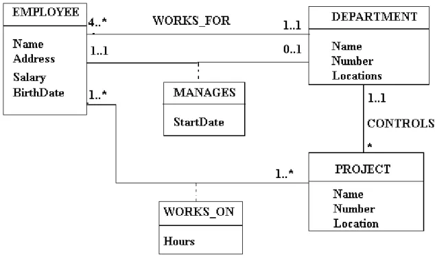
In any data model it is important to distinguish between the description of the database and the database itself. The description of a database is called the database schema, which is specified during database design and is not expected to change frequently. Most data models have certain conventions for displaying the schema as diagrams. For example, a preliminary database schema for the COMPANY database, derived from the previous description, may be displayed as in the figure 1. 1.
The diagram displays the structure of each record type but not the actual instances of records.
The actual data in a database may change quite frequently. For example, the employees, the salaries, the projects, etc. The data existent in a database at a particular moment in time is called a database state or snapshot. Figure 1. 2 illustrates a possible state of the COMPANY database.
The distinction between the database schema and a Database State is very
important. When we define a new database, we specify its database schema only to the DBMS. At this point, the corresponding Database State is the empty state, with no data.
The initial state of a database is the state after the database is first populated or loaded with initial data. Every time an update operation is applied to the database, we get
another Database State. At any point in time, the database has a current state. The DBMS is partly responsible for ensuring that every state of the database is a valid state-that is, a state that satisfies the structure and constraints specified in the schema.
Figure 1.1. Preliminary schema diagram for the COMPANY database.
Figure 1. 2. A state of the COMPANY database.
The architecture of a database can be described at three levels of abstraction (see figure 1.3):
1. The internal level
An internal schema describes the physical storage structure of the database. The internal schema uses a physical data model and describes the complete details of data storage and access paths for the database.
2. The conceptual level
A conceptual schema describes the structure of the whole database for a community of users. The conceptual schema hides the details of physical storage structures and concentrates on describing entities, data types, relationships, user operations and
constraints. A high-level data model or an implementation data model can be used at this level.
Figure 1. 3. The three-schema architecture.
3. The external or view level
This level includes a number of external schemas or user views. Each external schema describes the part of the database that a particular user group is interested in and hides the rest of the database from that user group. A high-level data model or an implementation data model can be used at this level.
1.2. A Database application Design
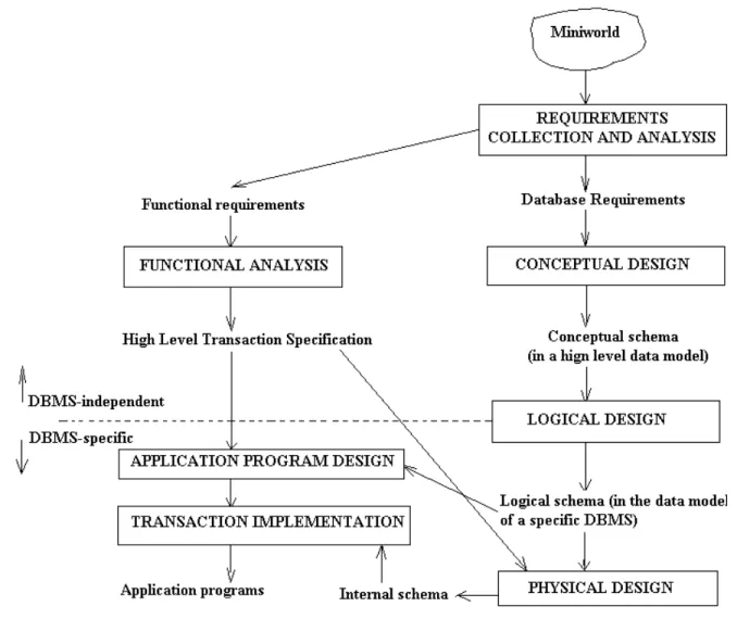
Figure 1. 4 shows a simplified description of a database application design process. This process begins after the Requirements Collection and Analysis. During this first step, the analyst interview prospective database users to understand and document their data requirements. The result of this state is a concisely written set of users’ requirements. These requirements should be complete and enough detailed.
In parallel with specifying the data requirements, it is useful to specify the known functional requirements of the application. These consist of the user-defined operations (or transactions) that will be applied to the database, and they include both retrievals and updates.
Once all the requirements have been collected and analyzed, the next step is to create a conceptual schema for the database, using a high-level conceptual data model.
This step is called conceptual design. The conceptual schema is a concise description of the data requirements of the users and includes detailed descriptions of the entity types, relationships and constraints. These are expressed using the concepts provided by the high-level data model. Because these concepts do not include implementation details, they are usually easier to understand and can be used to communicate with nontechnical users. A high-level conceptual schema can also be used as a reference to ensure that all users data requirements are met and that the requirements do not include conflicts. This approach enables the database designers to concentrate on specifying the properties of the data, without being concentrated with storage details.
The next step in database design is the actual implementation of the database, using a commercial DBMS. Most current commercial DBMSs use an implementation data model-such as the relational or the object database model-so the conceptual schema is transformed from the high-level data model into the implementation data model. This step is called logical design or data model mapping and its result is a database schema in the implementation data model of the DBMS.
Figure 1.4. The main phases of a database application design.
Finally, the last step is the physical design phase, during which the internal storage structures, access path and file organizations for the database files are specified.
In parallel with these activities, application programs are designed and implemented as database transactions corresponding to the high-level transaction specifications.
1.3. The Entity-Relationship Model
The Entity-Relationship Model is a popular conceptual data model.
1.3.1. Entities and attributes
An entity is a „thing“ in the real world with an independent existence. An entity may be an object with physical existence – a particular person, a car, an employee- or may be an object with a conceptual existence – a company, a job, a university course. Each entity has attributes – the properties that describe it. For example, an employee entity, in the COMPANY database design, may be described by the employee’s name, address, salary, birth date, the department to which he/she is assigned, the projects he or she is working.
A particular entity will have a value for each of its attributes. The attribute values that describe each entity become a major part of the data stored in the database. For example, the attribute values of a particular employee entity can be: „Judy Clark“, „Rosenweg 13“,
„25K“, „12.03.1970“, „01“, „01 (20)“ (see figures 1.1, 1.2).
Entity Types and Entity Sets
A database usually contains groups of entities that are similar. For example, a company employing hundreds of employees may want to store similar information concerning each of the employees. These employee entities have the same attributes, but each entity has its own value for each attribute. An entity type defines a collection (or set) of entities that have the same attributes. Each entity type is described by its name and attributes. The collection of all the entities of the same type is usually referred to using the entity type name. Ex: EMPLOYEE refers to both a type of entity as well as the current set of all employee entities in the database.
Key attributes of an Entity Type
An entity type usually has an attribute whose values are distinct for each individual entity in the collection. Such an attribute is called a key attribute, and its
values can be used to identify each entity uniquely. For example, the „number“ attribute of the „Department“ entity type can be used as a key attribute because no two
departments are allowed to have the same number. Sometimes, several attributes together form a key, meaning that the combination of the attribute values must be distinct for each entity.
1.3.2. Relationships
In an initial phase of the COMPANY database conceptual design, three types of entities were defined: EMPLOYEE, DEPARTMENT and PROJECT. These are
represented together with their attributes, in the preliminary schema diagram from the figure 1. 1.
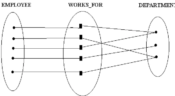
There are several implicit relationships among these entity types. In fact, whenever an attribute of one entity type refers to another entity type, some relationship exists. For example, the attribute ControllingDepartment of the PROJECT refers to the department that controls the project. Department of the EMPLOYEE refers to the department for which the employee works, and so on. In the ER model, these references should not be represented as attributes but as relationships. For example, we can define a relationship type WORKS_FOR between the entity types EMPLOYEE and
DEPARTMENT, which associates each employee with the department the employee works for (see figure 1. 5).
The WORKS_FOR relationship is of type N:1, or many to one, because it associates one or more employees with one department.
Suppose each employee can be associated with many departments. In this case, the relationship, lets name it WORKS_FOR_MANY is of type M:N, or many to many (see figure 1. 6).
Figure 1. 5. The WORKS_FOR relationship (many to one)
Figure 1. 6. The WORKS_FOR_MANY relationship (many to many).
Each employee works on many projects and many employees can work on the same project. The relationship WORK_ON, between the entity types EMPLOYEE and PROJECT is of type many to many (figure 1. 7).
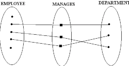
Each department has a unique employee that is the manager. The relationship MANAGES (figure 1.8), between the entity types EMPLOYEE and DEPARTMENT is of type 1:1 (one to one). Other types of relations are of type min:max. For example, 0:N, 1:10, 4:M, etc
Figure 1. 7. The WORK_ON relationship (many to many).
Relationships with attributes
An employee starts managing a department at a certain date. The starting date is an attribute of the relation between an employee and a department. This relationship, MANAGES, is of type 1:1. For this reason, the relationship attribute StartDate can be represented also, either as an EMPLOYEE attribute, either as a DEPARTMENT attribute.
For a 1:N relationship type, a relationship attribute can be migrated only to the entity type at the N-side of the relationship. For example, the relationship WORKS_FOR
Figure 1. 8. The MANAGES relationship (one to one).
can have an attribute StartDate, indicating when an employee started to work for a department. This attribute can be included as an attribute of the EMPLOYEE.
For M:N relationship types, some attributes may be determined by the combination of participating entities, not by a single entity. Such attributes must be specified as
relationship attributes. An example is the attribute Hours of the relationship WORK_ON.
An employee works a different number of hours to each project. The number of hours an employee works on a project is determined by an employee-project combination and not separately by either entity.
1.3.3. The Entity Relationship diagrams
There are many types of notations used to represent entities and relationships.
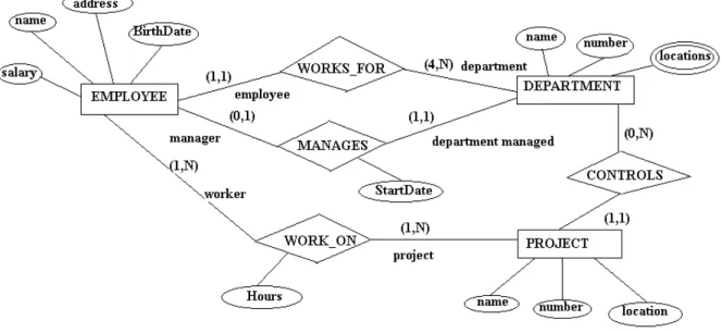
Examples of such notations are exemplified in the figures 1. 9, 1.10 and 1.11. Figure 1.10 adds the attributes to each entity type. Figure 1.11 is an equivalent representation in the Unified Modeling Language, which is now a de facto standard for software systems modeling.
Figure 1.9. ER diagram of the COMPANY database.
Figure 1.10. ER diagram of the COMPANY database, with attributes.
Figure 1. 11. The UML model of the COMPANY database.
1.4. Implementing an Entity Relationship model as a Microsoft Access data model
1.4.1. Entities representation
In the Microsoft Access data model, the set of all existent entities of a given type is represented by a table. You can give the table the entity type name. For example, the COMPANY database will contain at least 3 tables: EMPLOYEE, DEPARTMENT, PROJECT.
Each entity from a table is displayed on a row (see figure 1.12. a). It is a record of the table. All the rows have the same fields, which are displayed as the table columns.
Each entity attribute is represented by a field. The particular values of the attributes of an entity are displayed on a row, as the values of the fields.
The Datasheet View of a table displays the entire content of the table, at the current moment.
Figure 1.12. a. The datasheet view of the EMPLOYEE table.
The Design View of a table displays the attributes -that is, the fields- and the data type of each attribute (figure 1.12. b).
Figure 1.12. b. The Design View of the EMPLOYEE table.
The attribute key of an entity type is named primary key of the table. In the diagram from figure 1.13, the primary keys are displayed by bold characters.
1.4.2. Relationships representation
The one-to-many relationship is the most common type of relationship in a relational database. It can be directly represented in Microsoft Access. To create such a relationship, we add the field that contains the primary key on the „one“ side of the relationship to the table on the „many“ side of the relationship. For example, the department number, which is declared as the primary key in the DEPARTMENT table, appears as a field in the table EMPLOYEE (see figure 1.13).
In a many-to-many relationship, a record in a table A can have more than one matching records in table B and a record in table B can have more than one matching records in table A. This type of relationship cannot be directly represented in the
Microsoft Access data model. The problem is solved by creating a third table that breaks down the many-to-many relationship into two one-to-many relationships. We put the primary key from each of the two tables into the third table. For example, to represent the relation WORK_ON in the COMPANY database, we introduced the table named
EmployeesProjects, which contains all the links employee-project and associate to each link the relationship attribute, Hours.
In the conceptual design, the locations of each department are represented by an attribute of the DEPARTMENT entity. A project has only one location, which was represented by an attribute of the PROJECT entity. A project can have the same location as a department. For this reason, it is convenient to represent the locations in a separate table. In this way, any modification of a location that is a department location and a project location is made only in one place.
Figure 1.13. Relationships between the COMPANY database tables.
In a one-to-one relationship, a record in table A can have only one matching record in table B and a record in table B can have only one matching record in table A.
This type of relationship is unusual because in many cases the information in the two tables can simply be combined into one table. For example, to represent the relationship MANAGES we introduced a field IsManager in the EMPLOYEE table, with possible values Yes/No and the relationship attribute StartDate was represented by a field in the DEPARTMENT table. Another possibility is two introduce a field ManagerID in the DEPARTMENT table and to create a one-to-one relationship between the tables DEPARTMENT and EMPLOYEE.
1.4.3. Rules of Databases Normalization
The translation of an Entity-Relationships model into a set of correlated database tables is not so directly as it may seem at the first glance.
The normalization is the process of creating and relating tables according to a fixed set of rules. The most important three are the following:
All fields should be atomic, meaning that the data can’t be divided any further.
All fields in a table must be related to a primary key. A primary key field contains a unique value for each record.
All fields must be mutually independent, meaning that no field depends on the information in any other field in the same table.
The first rule
Let’s consider the Name attribute of the Employee type. Based on the first rule, this attribute was represented by two fields in the EMPLOYEE table: FirstName and LastName. If the name is represented in a single field it is very difficult to sort the table by last name or to query the table by the employees last name. If we are interested to query the EMPLOYEE table by some parts of the address (the country, the town) then the address must be broken in more fields, like the country, the town, the street, etc.
Another concern is repetitive data in a single field. For example, consider we represent the Locations attribute of the DEPARTMENT entity type by a field containing the list of locations. In this case it would be very difficult to do operations based on a particular location. A second solution would be to have several location fields, Location1, Location2, Location3, etc. But in this case we must limit the number of locations and many records will have empty fields because not all the departments have the same number of locations. The best solution is to create a table containing all the locations.
This is the Locations table in the COMPANY database. The number of records of the table is not limited. We introduced in this table a field containing the department number, which is the primary key in the DEPARTMENT table.
The second rule
This rule requires each table to have a primary key. A primary key is usually a single field that provides a unique identification of each record. A primary key can be composed of more fields. In all operations involving the primary key, Access considers all the fields declared as primary key.
The third rule
Sometimes, this rule is difficult to discern. The trick to finding dependent fields is to consider changing the data. If that change affects any other data in the same table, a problem exists. For example, if a table contains the fields price per unit, quantity and total sum, then the field total sum depends of the field quantity and also of the field price per unit. The field total sum must be eliminated. The total sum can be obtained by a query of the table.
Relationships and Data Protection
Relationships help to protect the data in tables. For example, you cannot delete a record from the DEPARTMENT table if there are records in the EMPLOYEE table, containing the department number from that record.
Two tables are related based on a primary key and a foreign key. For example, the DEPARTMENT table is a parent table that contains a primary key, DeptNumber. The EMPLOYEE table is a child table that inherits the primary key as a foreign key. Then, DeptNumber is a foreign key in the EMPLOYEE table.
1.4.4. Referential Integrity
Referential Integrity is another set of rules that Access uses to protect the relationships between related tables. Referential integrity ensures that the relationship is valid and that you don’t accidentally corrupt your data by adding or deleting records inappropriately.
Here are the conditions that referential integrity checks for:
Primary key fields must contain unique entries
Related fields must be the same data types.
Tables must be in the same database or be linked.
You can’t enter a value in a foreign key before entering it in the primary key field
You can’t delete a record from a parent table if a matching record exists in a related (child) table.
You can’t change the primary key value in the parent table if that record has related records.
1.5. Refining the Design
The last step of a database design is to analyze the design for errors. This is done by loading the database with some sample data and then verify if the results obtained from tables are correct. These first results enable to make some adjustments and
refinements to the initial design. It is easy to change the design of a database before the database is created. It becomes much more difficult to make changes to tables after they’re filled with data and after you have built forms and reports.
1.6. Objects and Naming Conventions
The Access objects are tables, forms, queries and reports.
Naming conventions are rules we are applying when we name the application objects, that is: tables, queries, forms, reports, macros and others. One naming
convention, which is common in Windows programming, is the Hungarian convention.
Based on this convention an object name is prefixed with the object type. For example, we can use the following prefixes:
tbl – for tables
qry – for queries
frm- for frames
rpt – for reports
For example, tblEmployee could be the name of a table, rptEmployee-the name for a report, etc.
1.7. The Northwind Database
This database is provided as a sample with the Microsoft Access installation kit.
We will use it in many examples of queries, forms and reports.
The database contains data about the sales of a company, its employees and customers. The aim of the database is to keep track of the sales orders, products, suppliers and customers.
A sale order contains data such as:
- the employee which emitted the order;
- the list of products ordered;
- the order date;
- the customer;
- the destination country, and others.
For each product the database must register:
- the type of the product;
- the unit price;
- units in stock;
- the suppliers, and others.
In the mini-world of this database may be identified four types of entities:
- employees;
- customers;
- products;
- suppliers;
- orders;
The job of an employee is to emit sale orders. An employee emits more orders. Then, an employee entity can be linked to many order entities at a time. Then, the relationship between the entity types Employee and Order is a one-to-many relationship.
A product may have many suppliers. The relationship between the entity types Product and Supplier is also a one-to-many relationship.
A customer may appear in many sale orders. Then, the relationship Customer-Order is of type one-to-many.
By an order can be sold many products, each of them in a different quantity.
A product may appear in many orders. Therefore, the relationship between the entity types Order and Product is a many-to-many relationship.
As we have seen, each entity type identified in the conceptual design phase is represented by a table, in the logical design. The table will contain all the entities of that type, existent at a moment.
In the logical design phase of the database it was necessary to break the many-to many relationship in two one-to-many relationships. This led to a new table, named
“OrdersDetails”, which contains the information on each product asked in an order.
In the detailed design phase other two tables were defined:
- “Categories”, necessary to store the characteristics of each product type;
- “Shippers”, to store details about the companies that may assure the products transport by ship.
The final result of the logical design is represented in the figure 1.14.
Figure 1.14.
You can analyze each table of the database:
Open the Database
Open each table:
o in Design View, to examine the type of each data field;
o in Datasheet View, to see the actual content of the table.
For example, the figures 1.15.a and 1.15.b show the table “Orders” in the Design View and in the Datasheet View.
Figure 1.15.a. The Design View of the table Orders Details
Figure 1.15.b. The Datasheet View of the table Orders Details
Chapter 2. Queries
The real power of a database is the ability to see the data it contains as we want, in the order and grouped as we want, to make analysis and calculations using that data.
By queries we can ask questions about the data in a database. For example, we can query the Northwind database to see what are the German customers, or which salesperson sold the most units of a given product.
Queries allow us to view and analyze our data in different ways:
Sort records by fields or by groups.
View records that meet specific criteria.
Perform calculations on groups of records.
Combine tables and other queries.
Create a database
To exercise with queries, which will be discussed in the following, we need a database. We can create very quickly our own database by importing tables from the Northwind database. Follow the steps:
Create a blank database.
Import from the Northwind database the tables: Employees, Orders and Customers (see figure 2.1).
Figure 2.1. Create a new table by importing it from another database.
Edit the relationships between the three tables:
o Choose the Relationships command from the Tools menu, to open the Relationships Window
o To specify the relationship between two tables, drag the foreign key from the child table to the primary key in the parent table. For example, to add the relationship between the Orders table and Customers table, drag the CustomerID field from the Orders table to the CustomerID in the Customers table (figure 2.2).
Figure 2.2. Editing the relationships between tables.
o Mark in the dialog box that is displayed after the dragging operation (figure 2.3) the option „Enforce Referential Integrity“ and press Create.
To obtain information about the three Integrity options, put the mouse cursor on the option and press the right button.
Figure 2.3. Create a relationship.
o The new relation will be displayed (figure 2.4).
Figure 2.4.
To see the properties of a relationship or to modify it, double-click on the relationship line. To delete or edit a relationship, put the cursor on the relationship line and then press the right button.
2.1. Create queries using the Query Wizard
The simplest way to create a query is by using the Query Wizard.
The Query Wizard can generate four types of queries:
Simple Query
Crosstab Query
Find Duplicates Query
Find Unmatched Query
2.1.1. Simple queries
A Simple query retrieves data from specified fields. The fields may belong to one table or they may be selected from more related tables. Also, by simple queries we can obtain minimum and maximum values in a field, totals and averages. Also, the number of records retrieved by a query may be limited by different criteria.
Example 2.1.
Suppose we want to know the orders emitted by each employee, and for each order, the order date, the customer’s company name and country. Therefore, we need a query from three tables: Employees, Orders and Customers. These tables are correlated:
each record from the Order table contains an EmployeeID and a CustomerID. We create the query in the following way:
Ask a new query and select Simple Query Wizard (figure 2.5)
Figure 2.5. Create a Simple Query with Wizard.
Select from the Employees table the fields LastName and FirstName (figure 2.6).
Figure 2.6. Select the necessary fields from the Employee table.
Select OrderDate from the Orders table (figure 2.7)
Select CompanyName and Country from the Customers table (figure 2.8)
Enter the desired name for the new query.
The query is shown in figure 2.9.
Select Design View from the View menu (figure 2.10).
In the bottom part of this view is displayed the Query by Example grid (the QBE grid). In this view we can specify one or more criteria for the query. For example, we may want to obtain only the orders related to a specific company.
We will enter the company name as a query criterion for the Company Name field.
Select Datasheet View from the View menu. The new query is shown in figure 2.11. It is sorted by the order date. We can change the record order by specifying the sort option to the corresponding field in the QBE grid.
Figure 2.7.
Figure 2.8 .
Figure 2.9. The Datasheet View of the EmployeesOrders query.
Figure 2.10. The Design View of the EmployeesOrders query.
Figure 2.11. The Datasheet View of the EmployeesOrders query.
Now, suppose we want to see only the sales to Germany. We switch in the Design View and enter the name of the country in the Country field (figure 2.12). We see the desired list of records in the Datasheet View of the query (figure 2.13).
Figure 2.12.
Figure 2.13. The orders list to Germany.
You will learn more about how to specify criteria to one or more fields from the laboratory exercises 2 and 3.
Link to a database a table from an existent database
In the following example, we need another table from the Northwind database, the OrderDetails table. At the beginning of this chapter we created a database by importing tables from the Northwind database. In this way we created a copy of each imported table in our database.
We didn’t need to modify any of the imported tables. We don’t need also to modify the table OrderDetails, so let’s examine another way to use a table from an existent database.
Suppose we use the same table in two or more databases. Then, when it is necessary to update the table, it is more convenient to operate the modifications only once and not in each database that use it. If we import the table, then we must operate the modifications in each copy of it. If we have only one table, which is shared by more databases, then we make the modifications only once. To have a shared table we define it in one database and then we link it to each database that need it. Linking the tables instead of importing
them has another advantage: we save disk space! The only restriction on a linked table is that we may not change the design of the table in the database in which it is linked. Its structure can be modified only in the database that contains it.
To link a table from an existent database just selects the link option (figure 2.14), after you asked to add a new table to your database.
Figure 2.14. Link to the database a table from another database.
Example 2. 2. Summary, min, max and average calculations.
When one of the fields selected in a query contains a number or a currency, the Wizard displays a window by which we can ask the computing of a supplementary column, containing the sum, the average, the minimum or the maximum from the values of all the records of the same type. For example, we can query the OrderDetails table to obtain the total quantity of products specified in each order.
Create a new query and select the fields OrderID and Quantity from the OrderDetails table (figure 2.15).
Figure 2.15.
The Wizard will display the dialog box from the figure 2.16. Select the Summary option and then press the Summary Options... button.
Figure 2.16.
In the Summary Options dialog box (figure 2.17) it is displayed the field Quantity because it contains a value of type number. Mark the Sum option and then press the OK button. We obtain the query shown in the figure 2.18.a.
Figure 2.17.
Figure 2.18. a. Figure 2.18. b.
The Count Records in Order Details option (figure 2.17) returns the number of records that make up each total. The query will contain a new field showing the result of the count (figure 2.18. b).
2.1.2. Crosstab Queries
The query from the example 2.2 is actually a Totals query. A Totals query performs calculations on groups of records. For example, we can obtain a subtotal for a group or the average value for a group.
A crosstab query is just a more complex Totals query. It summarizes data in rows and columns.
A Crosstab query must contain three elements:
A column heading A summary field A row heading
Example 2.3.
Ask to create a new query and select Crosstab Query Wizard (figure 2.5).
In the displayed Dialog Box (figure 2.19) we must select the table or the query that contains the data necessary in the new query. Only one query or table can be used to obtain a Crosstab query.
Select the Orders table and then press Next.
In the next three windows we must select:
The row heading (figure 2.20).
The column heading (figure 2.21).
The field to be summarized in the query and the way to calculate the values (figure 2.22). We selected the field Freight and the function Sum.
The Sample part of the window shows a generic version of the query.
If you want to see Help information on Crosstab queries, select the Display Help on Working with the Crosstab Query option, in the last dialog box (figure 2.23).
The Datasheet View of the query is shown in the figure 2.24.
If you deselect the option „Yes, include row sum“ in the Dialog box from figure 2.22, then the second column of the query table, „Total of Freight“ will be omitted.
Figure 2.19.
Figure 2.20.
Figure 2.21.
Figure 2.22.
Figure 2.23.
Figure 2.24. A Crosstab Query.
The Total Of Freight field lists the total freight cost per day. The first row is a subtotal for each country – that’s why there’s no date in the Shipped Date field for that record.
2.1.3 Find Duplicates Queries
This query is useful to find the records that have the same value in a specified field.
For instance, all the employees with the same hire date, all the orders with the same order date, etc.
Example 2.4.
Ask to create a new query and select Find Duplicates Query Wizard (figure 2.5).
In the first dialog box (figure 2.25), select the Employees table, as the table in which you want to find the duplicates.
In the next dialog box (figure 2.26), select the field „Hire Date“, as the field used for finding the duplicates.
In the next dialog box (figure 2.27) you may choose other fields to be displayed. For example, First Name and Last Name.
The resulted query is shown in the figure 2.28.
Figure 2.25.
Figure 2.26.
Figure 2.27.
Figure 2.28.
2.1.4. Find Unmatched Queries
Suppose we have two related tables in a database. If the relationship between the two tables is not of 1-1 type, then not all the records from one table are related to records from the other table. For example, it is possible that not all the customers registered in the Customers table to appear in the Orders table. We can easily find these customers using an Unmatched query. Any missing CustomerID value in the Orders table indicates customers with no orders.
Example 2.5.
Ask to create a new query and select Find Unmatched Query Wizard option.
Select Customers, as the table where to find records which have not related records in the other table.
Select Orders, as the table in which to find related records.
In the next dialog box you must specify the related fields in the two selected tables. The Wizard identified the two fields: CustomerID. You can change this field in either table if necessary. The selected fields must have the same data type.
In the next dialog box you can specify the fields to be displayed in the query.
For example, we want to see the company’s name and phone number for any customer that doesn’t have an order. Then, we select the CompanyName and Phone fields.
We obtain the query showed in the figure 2.29.
Figure 2.29.
2.2. Create queries without a Query Wizard
Although the Queries Wizards offer a fast way to produce different types of queries, the most flexible way to create a query is to design it without the Query Wizard.
Details about the editing of queries in Design View are presented in the laboratory lesson number 4.
Example 2.6. A calculation query for Inventory
In this example we will see how to create a query with calculation fields.
Suppose we want to have an inventory of the products in stock, that is for each product the inventory value is calculated as UnitPrice * UnitsIn Stock. We need a separate column to display the inventory values.
We ask to create a New query.
In the dialog box from figure 2.30 we select Design View.
Figure 2.30.
The next dialog box (figure 2.31) enables the selection of tables necessary for the new query. We select Products.
Figure 2.31.
We drag the field ProductName from the table to the Field row on the first column in the QBE (figure 2.32).
We type the calculation expression on the second column in the Field row. The calculation is expressed as: Inventory Value:[UnitPrice]*[UnitsInStock].
Figure 2.32.
We press the Run button in the Toolbar or ask the Datasheet View from the View menu. We obtain the query as in figure 2.33.
Figure 2.33.
As you can see, the calculation expression begins with the name of the calculation field followed by semicolon and then an arithmetic expression in which the operands are values from two fields of the Products table. The value in a field can be included in a calculation by enclosing the field name between square brackets.
You will learn more about calculations in queries from the LAB 3 exercises.
2.3. The Expression Builder
The Expression Builder is a very useful tool, which can be used to construct very complicated expressions in a graphical manner.
Expressions are combinations of values, constants, functions, fields and operators that can be evaluated to a single value.
The Expression Builder can be started by right clicking in any Criteria or Field row of a query, when the query is opened in Design View (figure 2.34). Select Build…
option from the pop-up menu. The Expression Builder dialog box will appear like the one shown in figure 2.35.
Figure 2.34.
The empty window at the top of the dialog box is used to display an expression, which can be typed directly in this window or can be constructed graphically by using the Expression Builder.
The bottom half of the Expression builder is an area containing three boxes that collectively contain all the expression elements available in Access 97.
The left box lists the folders that contain all the database objects (tables, queries, forms and reports), built-in and user-defined functions, constants, operators and common expressions.
The middle box lists specific elements or categories of elements for the folder selected in the left box. For example, if we select Built_In functions in the left box, then the middle box will display all the categories of Access built-in functions (figure 2.36).
The right box contains the values for the selected elements in the left and middle box (see figure 2.36).
Figure 2.35.
Figure 2.36
To create an expression, select each operand and operator and use Paste button to transfer it in the Expression window. When you press OK the current expression is copied in the place from where the Expression Builder was started, for example in the Criteria field.
To construct several criteria, start the Expression Builder separately for each field. For example, imposing the two criteria from the figure 2.37, the query will contain only the products having a unit price greater that 10 and which were sold in a quantity less than 100.
Figure 2.37
Example 2.7.
Constructing a query that uses a calculated date as a criterion with Expression Builder.
We want to build a query that returns the set of customers that had orders in the year 1997 and whose orders in that year took longer than 15 days to process from receiving the order to shipping the order.
Start a new query in Design view (figure 2.30).
Select the tables to use in query. In our example these will be Orders and Customers.
Drag the necessary fields from the two tables in the QBE grid (figure 2.38)
To obtain the specified result we have to assign a criterion to both the OrderDate and the ShippedDate fields.
Figure 2.38
Start the Expression Builder from the Criteria row of the OrderDate column.
Make the selections as in figure 2.39 and double-click Year.
Select the Orders table in the left box and OrderDate Field from the middle box.
Select the placeholder from the expression and then double-click <Value>
to replace it with the value from the OrderDate field.
Click the = button and type 1997 into the Expression box. The expression looks like in figure 2.40.
Click OK.
Figure 2.39
Figure 2.40
Follow the same steps to build the criterion for the ShippedDate field.
Double-click the DateAdd function. The expression should appear like the one shown in figure 2.41. The DateAdd function enables to calculate a date by adding a specified time interval to that date.
Figure 2.41.
Replace the placeholders (see figure 2.42):
o interval by “d”, meaning “days”;
o number by 15
o date, by the value contained in the OrderDate field
Because we want to find all orders that were processed in more than 15 days we need to add the greater than sign in front of our expression (figure 2.43).
The result should be like in figure 2.44.
Figure 2.42.
Figure 2.43.
Figure 2.44.
Chapter 3. Form Basics
Forms are objects used to interact with a database. They can help in viewing, entering and modifying data. Forms are also parts of the applications user-interfaces. To understand better what are the forms, we will begin with the Wizard generated forms.
The Access’s form wizards use different defaults to generate forms based on tables and queries. There are two types of Form Wizards:
AutoForms
Form Wizard
The AutoForms are specific types of forms, containing all the fields of a table or of a query. The Form Wizard allows selecting the fields to be included in a form.
The Form Wizards generate four types of forms:
Columnar – each record is displayed on one column, with each field on a separate line. Typically, this form displays one record at a time (see figure 3.2).
Tabular – each record is displayed on a row, in a column format. This is a good format for displaying multiple records (see figure 3.3).
Datasheet – this is the table format used to display the tables and queries when the database is opened. Displaying the data in such a form doesn’t need to open the database (see figure 3.4).
Justified – This form distributes the controls in which are displayed data evenly between right and left margins and top and bottom margins. This type of form is available only with the Form Wizard (see figure 3.8).
3.1. The AutoForm Wizard
To create an AutoForm with the Wizard, follow the steps:
Ask to create a new form.
From the „New Form“ dialog box (figure 3.1) select the table or query to display and one of the three AutoForm formats and then click OK.
The new form is generated. For example, the form generated using the settings from the figure 3.1 is shown in the figure 3.2. The picture displays only the first record of the
Orders table. To see other records use the buttons located the bottom of the form. To add a new record go to the end of the table using the rightmost button and then enter the corresponding value in each field.
Repeat the above steps for the same table but using the other two auto formats. The Tabular and Datasheet forms are shown in figure 3.3 and 3.4
Figure 3.1. Create an AutoForm.
Figure 3.2. A columnar form.
Figure 3.3. A tabular form.
Figure 3.4. A Datasheet form.
3.2. The Form Wizard
The Form Wizard offers the three previous form styles and also the justified type. But more important is that with this wizard we can choose the fields to be included in a form.
Let’s create a justified form with the Form Wizard.
Ask to create a New form
Select Form Wizard from the New Form dialog box.
Select the table / query and the fields to be displayed in the form (figure 3.5).
Figure 3.5.
Choose justified option from the Form Wizard dialog box (figure 3.6).
Figure 3.6.
Choose one of the styles to display the form (figure 3.7) and give it the desired name.
Figure 3.7.
Figure 3.8. shows the form obtained using the settings from the figures 3.5 and 3.6, in the Standard style. Try with different styles of displaying offered by the Form Wizard.
Figure 3.8. A Justified form.
When the form is created starting from more that one tables/queries, you may choose between obtaining a single form containing all the selected fields or a form with subforms.
3.3. The Chart Wizard
Sometimes it is very useful to have a graphical representation of the dependency between some data in a table. The Form Wizard can generate such graphically
dependencies as different types of charts. Usually, these charts are added to existing forms or reports.
Example 3.1.
Ask to create a New form, select the table and the Chart Wizard option (figure 3.9).
Figure 3.9.
Select the fields to use for the chart (figure 3.10).
Select the type of chart you want (figure 3.11).
In the next dialog box (figure 3.12):
o You can see a preview of the chart:double-click the button from left-top corner of the window.
o You can drag and drop the field controls to change the wizard orientation.
o You can change the grouping of data –by, year, by quarter, by month, etc.
o You can change the calculation options.
Try every one of these variants.
The chart form generated by the Wizard using the settings from the figures 3.10, 3.11 and 3.12 is shown in the figure 3.13.a.
Figure 3.10.
Figure 3.11.
To edit the chart double-click on the chart. The datasheet of the diagram is displayed as in the figure 3.13.b.
Figure 3.12.
Figure 3.13.a. Figure 3.13.b.
Example 3.2. Adding a Chart to an Existing Form
Open the form in which you want to insert the chart. We will use a form (figure 3.14) that displays a query, qryQuantityByMonth. The query was created from the tables Orders-fields CustomerID and OrderDate- and OrderDetails-field Quantity.
I asked to obtain the Sum of the values from the Quantity field and the grouping of records by months.
Figure 3.14.
Choose Design View from the View menu.
Choose Chart from the Insert menu.
Click inside the form where you want to position your chart.
Follow the procedure to create a chart. In this example we created a chart starting from the same query, qryQuantityByMonth. Figure 3.15 explains the chart.
The next dialog box (figure 3.16.) gives you the opportunity to link your chart to the existing form data.
Choose Form View from the View menu. The chart is shown in the figure 3.17.
Change the record number using the control from the bottom part of the window, to see the synchronous updating of the document and the chart.
Figure 3.15.
Figure 3.16.
Figure 3.17.
Chapter 4. Reports
A report is a printed hard copy of some data of a database, presented in a
particular format. A report is based on a table or a query, but the data can be presented in any fashion we need.
A report (see figure 4.1) usually has a header at the beginning of the report, which normally contains the title of the report and other introductory information. It also has footer, at the end, which contains final results like grand totals.
Each page can have a header and footer. The page header contains the column headings. The page footer typically contains the page number.
A report can be designed “manually” or using a Report Wizard. To design it
“manually”, ask to create a new Report and then choose Design View from the List Box in the dialog from the figure 4.2. You will have to create the layout item by item. This can be a very tedious operation. A much easier solution is to use the Report Wizards.
Figure 4.1.The format of a report.
The Report Wizards
Many types of reports can be generated using the Report Wizards. If one of these types of reports is convenient for you, then you can save time creating reports with the Wizard. Also, you can generate a report using the Wizards and after that, change the design of the report in any desired way.
The Report Wizards are similar to the Form Wizards in that there are two types:
The AutoReports
The Report Wizard There are three types of reports:
Columnar - the report displays data in one column, with each field on a separate line.
Tabular - the report displays all the data from one record in the same row – each field in a separate column.
Justified – The data are distributed evenly between the right and left margins and the top and bottom margins.
4.1. Creating AutoReports
The AutoReports Wizard automatically generates a specific type of report, using all the fields in the specified table or query.
Example 4.1.
Ask to create a New report.
From the New Report dialog box (figure 4.2.), select the table or the query you want to print in the report. Choose AutoReport: Columnar or AutoReport:
Tabular.
The new report is generated.
o Click on the left button when the cursor is on the report surface, to view the print preview.
o Click on the right button: you can see more that one page at different levels of zoom.
Figure 4.2.
4.2. Using the Report Wizard
The Report Wizard is a little more flexible than the AutoReport Wizard in that it allows you to select the fields you want to report on. Also, it offers a third style – justified.
Because you have the possibility to see how are the columnar and the tabular forms, let’s examine how to use the Report Wizard to obtain a justified report. It is similar in style to a justified form.
Example 4.2.
Ask to create a new report.
Double-click Report Wizard in the New Report dialog box.
Select the fields you want to include (figure 4.3). In this example I selected fields from four related tables: Customers, Orders, Order Details and Products.
Select the table that you want to be used as starting point in report generation (figure 4.4). For example, selecting the Orders table, the Wizard will traverse the Order table and for each record from this table will search the related data in the other tables. The right part of the dialog box shows you a preview of the report. Select one by one each of the tables listed in the left part to see the preview of the report.
Figure 4.3.
Figure 4.4.
The next dialog box enables to change the grouping of data and the priority of levels. For example, the figure 4.5. shows the grouping generated by the
Wizard. Using the “>” button and the priority buttons I changed the levels and the grouping of data as in the preview from the figure 4.6.
Figure 4.5.
Figure 4.6.
In the dialog box from figure 4.7, you can choose the fields used for sorting the records in the report. Also, using the Summary Options you can ask to include in the report a field’s total, its average, and its minimum or maximum value.
Try different styles of lay out from the next dialog box (figure 4.8). The lay out is represented in the left window of the dialog box.
Figure 4.7.
Figure 4.8.
Figure 4.9.
Figure 4.10. shows the report that was generated based on grouping from the figure 4.5.
Figure 4.10.
4.3. Creating a Chart Report
The procedure to create a chart report is very similar to that of creating a chart form.
Ask to create a new Report.
Select Chart Wizard (see figure 4.2) and the table or query to use in producing the chart. In this example we selected the Product table.
Select the fields you want to represent in the chart. We selected the Product Name and Units in Stock.
Select the type of chart you want (see figure 3.7).
Rearrange the defaults arrangements and calculations for the chart (see figure 3.8).
Choose the name of the chart.
Wizard generates a chart like the one in figure 4.11.
Figure 4.11.
4.4. Adding a chart to an existing report
The steps to add a chart to a report are very similar to those required to add a chart to a form.
Open the report in which you want to insert the chart, in Design View.
Select Chart from the Insert menu.
Click inside the report area where you want to insert the chart.
Follow the steps required to create the chart.
The Wizard allows you to dynamically link the chart to the current record. You can choose No Fields from the Report fields and Chart Fields drop-down lists if you don’t care to link the chart to the current record.
Figure 4.12 shows a report in which it was included a chart.
Figure 4.12.
Chapter 5. Customizing forms
When we want to quickly create a form with standard features, then the Form Wizards are very appropriate. Otherwise, we can create a form to satisfy the particular needs of an application, without the Form Wizards, or we can modify a Wizard generated form.
Forms are used to display data from a database, to enter new data or to modify the existent data. These output and input operations are performed using special windows called Controls. Figure 5.1 shows a form containing more types of controls:
text boxes, used to display and enter a single string;
list boxes and combo boxes, used to display lists form tables and queries or lists of arbitrary values;
command buttons;
option groups, and others.
Figure 5.1
A bound object is an object that is attached to a data source. That object can be a form, a report or a control. For instance, a form bound to a table will display the data in that table. The form can also be used to enter new data in the table or to modify the existing data in the table.
A table or a query to which is bound a form is called the form’s Record Source. It is chosen when the form is created, from the New Form dialog box.
The Record Source is a form’s property and is available through the form’s property sheet.
Figure 5.2. Select the Record Source of the new form.
Figure 5.3. A form property sheet.
5.1. Bound, Unbound, and Calculated Controls
A control can display data that is taken directly from the database, values that are calculated using more data from a database or values entered by a user.
A control whose source of data is a field in a table or query is a bound control. The bound controls are used to display, enter and update values from fields in a database. The values can be text, dates, numbers, Yes/No values, pictures or graphs. The text box is the most common type of bound control. For example, the text boxes that display the Product Name and the Unit Price from the fields of the Product table (figure 5.5) are bound controls.
The field to which is bound a control is called the control’s Control Source. The field must belong to the table or query that is the Record Source of the form. It is available through the control’s property sheet. The figure 5.4 shows the property sheet of the text box that displays the Product Name in the form from figure 5.5.
Figure 5.4. A control property sheet.
A control whose source of data is an expression rather than a field is a calculated control. For example, the text box that displays the discounted price, calculated with the formula Unit Price *0.75 is a calculated control. A calculated control displays data – the result of its expression – but that control isn’t bound to a table or a query. In other words, it displays data but doesn’t store it.
A control that doesn’t have a source of data (a field or expression) is an unbound
control. Such controls are used to display information, lines, rectangles and pictures. For example, the three controls that label the text boxes are unbound controls.
Figure 5.5
Using the Toolbox
The Toolbox is a toolbar specialized for controls. It is displayed automatically when a form is opened in Design View. The meaning of each graphical symbol from the Toolbox is shown when you put the cursor on the symbol surface. The general procedure to create a control is: click on the corresponding button in the Toolbox and then click on the place in the form where you want to put the control.
5.2. Text Boxes
A text box can be a bound control, an unbound control or a calculated control.
Creating a Bound Text Box
Open the form in Design View.
Display the Field List: click the Field List button or select Field List from the View menu.
Click on the Text Box button in the Toolbox.