Werner A. Stahel
Abstract
Reproducibility of quantitative results is a theme that calls for probabilistic models and corresponding statistical methods. The simplest model is a random sample of normally distributed observations for both the original and the replication data. It will often lead to the conclusion of a failed reproduction because there is stochastic variation between observation campaigns, or unmodeled correlations lead to optimistic measures of preci- sion. More realistic models include variance components and/or describe correlations in time or space.
Since getting the “same circumstances” again, as required for reproducibility, is often not possible or not desirable, we discuss how regression models can help to achieve credibility by what we call a “data challenge” of a model rather than a replication of data. When model development is part of a study, reproducibility is a more delicate problem. More generally, widespread use of exploratory data analysis in some fields leads to unreliable conclusions and to a crisis of trust in published results. The role of models even entails philosophical issues.
1 Introduction
Empirical science is about extracting, from a phenomenon or process, features that are relevant for similar situations elsewhere or in the future. On the basis of data obtained from an experiment or of a set of observations, a model is determined which corresponds to the ideas we have about the generation of the data and allows for drawing conclusions concerning the posed questions.
Frequently, the model comprises a structural part, expressed by a formula, and a random part. Both parts may include constants, called parameters of the model, that represent the features of interest, on which inference is drawn from the data. The simplest instance is the model of a “random sample” from a distributions whos expected value is the focus of interest.
The basic task of data analysis is then to determine the parameter(s) which make the model the best description of the data in some clearly defined sense.
The core business of statistics is to supplement such an “estimate” with a mea- sure of precision, usually in the form of an interval in which the “true value”
should be contained with high probability.
This leads to the basic theme of the present volume: If new data becomes
available by reproducing an experiment or observation under circumstances as similar as possible, the new results should be compatible with the earlier ones within the precision that goes along with them. Clearly, then, reliable precision measures are essential for judging the success of such “reproductions”.
The measures of precision are based on the assessment of variability in the data. Probability theory provides the link that leads from a measure of data variability to the precision of the estimated value of the parameter. For example, it is well known that the variance of the mean ofnobservations is the variance of the observations’ distribution, divided by nif the observations are independent.
We will emphasize in this chapter that the assumption of independence is quite often inadequate in practice and therefore, statistical results appear more precise than they are, and precision indicators fail to describe adequately what is to be expected in replication studies. In such cases, models that incorporate structures of variation or correlation lead to appropriate adjustments of precision measures.
Many research questions concern the relationship between some given input or “explanatory” variables and one or more output or “response” variables. They are formalized through regression models. These models even allow for relating studies that do not meet the requirement of “equal circumstances” which are necessary for testing reproducibility. We will show how such comparisons may still yield a kind of confirmation of the results of an original study, and thereby generalize the idea of reproducibility to what we calldata challenges.
These considerations presume that the result of a study is expressed as a model for the data, and that quantitative information is the focus of the repro- duction project. However, a more basic and more fascinating step in science is to develop or extend such a model for a new situation. Since the process of devel- oping models is not sufficiently formalized, considerations on the reproducibility of such developments also remain somewhat vague. We will nevertheless address this topic, which leads to the question ofwhat is to be reproduced.
In this paper, we assume that the reader knows the basic notions of statistics.
For the sake of establishing the notation and recalling some basic concepts, we give a gentle introduction in Section 2. Since variation is the critical issue for the assessment of precision, we discuss structures of variation in Section 3.
Regression models and their use for reproducibility assessment is explained in Section 4. Section 5 covers the issue of model development and consequences for reproducibility. Section 6 addresses issues of the analysis of large datasets.
Comments on Bayesian statistics and reproducibility follow in Section 7. Some general conclusions are drawn in the final Section 8.1
1While this contribution treats reproducibility in the sense of conducting a new measurement campaign and comparing its results to the original one, the aspect of reproducing the analysis
●
●
●
●
●
●
●
●
●
●
●
●
●
●
●
●
●
●
●
●
●
●
●
●
●
●
●
●
●●
●
●
●
●
●
●
●
●
●
●
●
●
●●●●
●
●●
●
●
●●
●
●
●
●●
●
●
●
●●
●
●
●
velocity [km/s] − 299.700
0 10 20 30 40 50 60 70 80
−1000100200300400500
984
"true"
day 1 day 2 day 3
−
t test
−
t without outliers
−
Wilcoxon
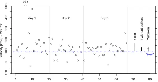
Figure 1: Measurements of the velocity of light by Newcomb in 1882. Three confidence intervals are shown on the right.
2 A Random Sample
2.1 Simple Inference for a Random Sample
The generic statistical problem consists of determining a constant from a set of observations that are all obtained under the “same circumstances” and are supposed to “measure” the constant in some sense. We begin with a classic scientific example: the determination of the velocity of light by Newcomb in 1882. The data set comprises 66 measurements taken on three days, see Fig. 1.
The probability model that is used in such a context is that of a random variableXwith a supposed distribution, most commonly the normal distribution.
It is given by a density f or, more generally, by the (“theoretical”) cumulative distribution function F(x) = P(X ≤ x). The distribution is characterized by parameters: the expected value µ and the standard deviationσ (in case of the normal distribution). For the posed problem, µ is the parameter of interest, and σ is often called a nuisance parameter, since the problem would be easier if it were not needed for a reasonable description of the data. We will useθ to denote a general parameter and θto denote the vector of all the parameters of the model. The distribution function will be denoted by Fθ(x).
of the data is left to Baileyet al. (this volume). The tools advocated by many statisticians to support this aim are the open source statistical system R and the documentation toolsSweave andknitr(Leisch 2002, Xie 2013, Stoddenet al. 2014).
−100 0 50 150 250 350 450
0246812162024
frequency
−100 0 50 150 250 350
0.00.20.40.60.81.0
F
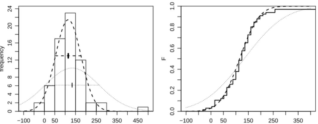
Figure 2: Histogram (left) and empirical cumulative distribution function (right) for the Newcomb data. The dashed and dotted lines represent normal distribu- tions obtained from fits to the data without and with two outliers, respectively.
If the model is suitable, the histogram describing the sample valuesx1, x2, ..., xn will be similar to the density function, and the empirical cumulative distribu- tion functionF(x) = #(xb i≤x)/n will be like the theoretical one (Fig. 2). For small samples, the similarity is not very close, but by the law of large numbers, it will increase with n and approach identity for n → ∞. Probability theory determines in mathematical terms how close the similarity will be for a givenn.
The question asked above concerns the mean of the random quantity. It is not the mean of the sample that is of interest, but the expected value of the random variable. It should be close to the sample mean, and again, probability theory shows how close the mean must be to the expected value. It thereby gives us the key to drawing statistical inferences about the model from the sample of data at hand – here, for inferences about the parameterθ.
The basic questions Q and answers A in statistical inference about a param- eter of a model are the following.
Q1 Which value of the parameterθ(or parameters θ) is most plausible in the light of the datax1, x2, ..., xn?
A1 The most plausible value is given by a functionθ(xb 1, x2, ..., xn)(orbθ(...)) of the data, called anestimator.
Q2 Is a given value θ0 of a parameter plausible in the light of the data?
A2 The answer is given by astatistical test. A test statisticT(x1, x2, ..., xn;θ0) is calculated, and the answer is “yes” if its value is small enough. The threshold for what is considered “small” is determined by a preselected probabilityα (called thelevel of the test, usually 5%) of falsely answering
“no” (called the error of the first kind). Usually, the test statistic is a
function of the estimatorbθof all model parameters and of the parameter θ0. If the answer is “no”, one says that the test is (statistically) signifi- cant or, more explicitly, that thenull hypothesis H0 that the parameterθ equals the supposed valueθ0 is rejected. Otherwise, H0 is not rejected – but not proven either; therefore, it may be misleading to say that H0 is
“accepted”.
The test statistic is commonly transformed to the so-calledp-value, which follows the uniform distribution between 0 and 1 if the null hypothesis is true. The test is significant if the p-value is belowα.
Q3 Which values forθ are plausible in the light of the data?
A3 The plausible values form the confidence interval. It is obtained by de- termining which values of θ are plausible, in the sense of Q2. Once the confidence interval is available, Q2 can therefore be answered by examining whetherθ0 is contained in it.
2.2 The Variance of a Mean
The basic model fornrandom observations is called thesimple random sample.
It consists of n stochastically independent, identically distributed random vari- ables. It is mathematically convenient to choose a normal distribution for these variables, which is characterized by its expected valueµand its varianceσ2 and denoted byN(µ, σ2). If we want to draw an inference about the expected value µ, the best way toestimate it from the data is to use the meanx¯=Pn
i=1xi/ n.
This answers Q1 above.
For answering the test question Q2, we use the result that under the as- sumptions made,
X¯ ∼ N(µ, σ2/n), (1)
where the notation means that x¯ is distributed as normal with expected value µand variance σ2/n. We first postulate thatσ is known – as may be the case when the variation of the observations can be assumed to be the same as in many previous experiments. Then,
P µ−1.96seX¯ <X < µ¯ + 1.96seX¯
= 0.05, where seX¯ =σ/√
n is called the standard error of the sample mean, and 1.96 is the 0.975-quantile of the normal distribution. This is the basis of answering Q2 by saying that µ0 is “plausible at the level α = 0.05” if x¯ is contained in the interval µ0−1.96seX¯ <x < µ¯ 0+ 1.96seX¯. Otherwise, the null hypothesis H0 : µ = µ0 is rejected. Finally, question Q3 is answered by the confidence
interval, which is written as [ ¯X−1.96seX¯, X¯ + 1.96seX¯]or, equivalently, as X¯ ±1.96seX¯.
In the more realistic case thatσis not known, it must be estimated from the data. This leads to modifications of the test and the confidence interval known under the notion oft-test. We refer to standard textbooks. For the example of the measurements of the velocity of light above we get X¯ = 134, leading to a velocity of299,834km/s, and a confidence interval of [102,166].
The assumption of a normal distribution for the observations is not very crucial for the reliability of the test and confidence interval. The central limit theoremstates that the sample mean is approximately normally distributed even if the distribution of the observations is non-normal, possibly skewed and mod- erately long-tailed (as long as the observations have a well-defined variance).
For heavily long-tailed, but still symmetric distributions, there is a nice model called thestable distribution. It contains the normal distribution as the limiting case. Except for this case, stable distributions have no variance (or an infinite one), but still a scale parameter. The mean of such observations has again a stable distribution (whence the name), but its scale parameter is proportional to n−γ with γ < 1/2 (where 1/2 corresponds to the normal distribution, see above). This means that there is a realistic model for which the standard error of the mean goes to 0 at a slower rate than under the normal model. Nevertheless, if standard methods are applied, levels of tests and confidence intervals are still reasonably valid, with deviations to the “safe side”.
Long tails lead to “extreme” observations, well known under the termoutlier.
The Newcomb dataset contains (arguably) two such outliers. Long tails are so widespread that the normal distribution for observations is often not more than wishful thinking. Although this does not affect the validity of the methods based on normal theory too much, it is preferrable to avoid means, but estimate or test parameters by alternative methods.
It is often tempting to disregard outliers and analyze the data without them.
In the example above, this results in the confidence interval[100,130]. However, dropping outliers without any corrective action leads to confidence intervals that are too short. Methods that deal adequately with restricting the undue influence of outliers (and other deviations from assumptions) form the theme of robust statistics. These methods are statistically more efficient than those based on the mean, in particular for pronounced long tails. An interval based on robust methods for our example yields[101,132].
For simple random samples, there are methods which avoid assuming any specific distribution, known as nonparametric procedures. These methods are robust and often quite efficient. Therefore, the t-test and its confidence interval
should not be applied for simple random samples. In such cases, a Wilcoxon signed rank test and the respective confidence interval (associated with the
“Hodges-Lehman estimator”) should be preferred. Our example yields an esti- mate of118and a confidence interval of[106,136]. The interval is much shorter than the t-interval for the whole dataset. It is as long as, but different from, the interval obtained without outliers or the robust interval.
The value corresponding to today’s knowledge,92, is not contained in either one of the intervals. We are lead to concluding that the experiments of Newcomb had a systematic “error” – a very small one, we should say.2
2.3 General Parameters and Reproducibility
Using the mean for inferences about the expected value of a distribution is the generic problem that forms the basis for inferences about a parameter in any parametric probability model. For a general parameter, the principle of maximum likelihood leads to an estimator. The central limit theorem yields an approximate distribution for it, allowing for approximate tests and confidence intervals. It relies on a linearization of the estimator. Refinements are needed for small sample sizes, robustness issues, and some special cases.
As to the issue of reproducibility, let us note that the confidence interval is supposed to cover the “true value” of the parameter, not its estimate (e.g., the mean) for the new sample. For testing the success of a reproduction, the difference of the parameter estimates should be examined. It has an approxi- mate normal distribution with variance equal to the sum of the variances of the parameter estimates. This yields a confidence interval for the true difference, which should contain difference zero for a successful reproduction.
2.4 Reproducibility of Test Results and the Significance Controversy
A statistical test gives a “yes” (accept) or a “no” (reject) for the null hypothesis H0 as its result. Reproducibility would then mean that a “yes” in an original study entails a “yes” in its reproduction; and a “no” entails another “no” in the reproduction.
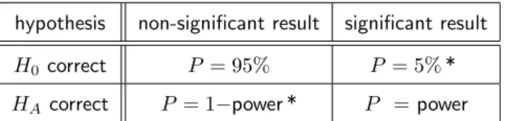
Table 1 collects the four possible cases determined by the validity of the
2Since 1983, the velocity of light isdefinedby the definition of the second and the meter, according to resolution 1 of the 17th Conf´erence G´en´erale des Poids et Mesures,www.bipm.
org/en/CGPM/db/17/1/. As a consequence, the velocity of light is exactly 299,792,458 m/sec and has become adefinedconstant in the SI system of units.
hypothesis non-significant result significant result
H0 correct P = 95% P = 5%*
HA correct P = 1−power * P =power
Table 1: The probabilities of getting the same result in the replication study, for the four possible cases of correct null hypothesisH0 and alternative hypothesis HA and significance of test results in the original study. * Replication of wrong results is undesirable.
hypothesis and (non-significant or significant) test results in the original study.
Assume first that the null hypothesis H0 is correct. Then, the probability for its acceptance is large (equal to 1−α, usually 95%) in both studies. Given that acceptance was reached in the first study, the probability of a succesful replication is 1−α. However, since H0 can never be “proven”, one merely obtains a further indication that there may be “no effect”. If the null hypothesis is rejected even though it is correct, we do not really want this to be replicated, and the respective probability is as low asα. Since one rarely wants to replicate a null result, such cases are less important. If the null hypothesis is wrong, the probability of getting rejection is equal to the power of the test and depends, among other things, on the sample size. Only in the case of good power for both studies, we obtain the same, correct result with high probability. Thus, test results are generally not reproducible.
These considerations are related to a major flaw of hypothesis testing: A potential effect that is subject to research will rarely be precisely zero, but at least a tiny, possibly indirect and possibly irrelevant true effect should always be expected. Now, even small effects must eventually become significant if the sample size is increased according to the law of large numbers. Therefore, a significance test indeed examines if the sample size is large enough to detect the effect, instead of making a clear statement about the effect itself.
Such arguments have lead to a controversy about “null hypothesis signif- icance testing” in the psychology literature of the 1990s. It culminated in a task force discussing to ban the use of significance testing in psychology journals (Wilkinson and Task Force on Statistical Inference 1999). The committee re- grettably failed to do so, but gave, among fundamental guidelines for empirical research, the recommendation to replace significance tests by effect size esti- mates with confidence intervals. Krantz (1999) presents a thorough discussion, and Rodgers (2010) and Gelman (2014) provide more recent contributions to this issue.
In conclusion, in spite of its widespread application, null hypothesis sig- nificance testing does not really provide useful results. The important role of a statistical test is that it forms the basis for determining a confidence interval (see Sec. 2.1). Results should be given in terms of confidence intervals for parame- ters of interest. The statistical test for no difference of the quantity of interest between the replication and the original study may formally answer whether the reproduction was successful. But even here it is preferrable to argue on the basis of a confidence interval for this difference.
The null hypothesis test has been justified as a filter against too many wild speculations. Effects that do not pass the filter are not considered worth mentioning in publications. The main problem with this rule is its tendency to pervert itself: Whatever effect is found statistically significant is regarded as publishable, and research is perverted to a hunt for statistically significant results. This may indeed have been an obstacle to progress in some fields of research. The replacement of tests and their p-values by confidence intervals is only a weak lever against this perversion. At least, it encourages some thought about whether or not an effect is relevant for the investigated research question and may counteract the vast body of published spurious “effects”.
A second problem of the filter is that it explicitly leads to the publication and selection bias of results, which is in the focus of this book as a mechanism to produce a vast body of spurious published effects or relationships, see Section 5.4 and Ehm (this volume, Sect. 2.4).3
3 Structures of Variation
3.1 Hierarchical Levels of Variation
Even if measurement procedures are strictly followed, ample experience from formal replications shows that the test mentioned in Sec. 2.1 too often shows significant differences between the estimated values of parameters of interest.
This experience is formally documented and treated ininterlaboratory stud- ies, in which different labs get samples from a homogeneous material and are asked to perform two or more independent measurements of a given property.
The model says that the measurements within a labh follow a (normal) distri- bution with expectationmh and varianceσ2, where the latter is assumed to be the same for all labs. The expectations mh are modeled as random variables
3Killeen (2005) proposed ameasure of replicationprep to overcome the problems with null hypothesis testing. However, since this measure is a monotonic function of the traditional p-value, it does not overcome the problems associated with significance testing.
from a (normal) distribution with the “true” value µas its expected value and a varianceσm2.
If there was no “laboratory effect” σm would be zero. Then, the precision of the mean of n measurements obtained from a single lab would be given by σ/√
n. Ifσm>0, the deviation of such a mean fromµhas varianceσm2 +σ2/n and obtaining more measurements from the same lab cannot reduce this variance belowσ2m.
When looking at an interlaboratory study as a whole, measurements from the same lab are more similar than those coming from different labs. This is called the within labs (or within groups) correlation. The term reproducibility is used in this context with a well-defined quantitative meaning: It measures the length of an interval that contains the difference of two measurements from different labs with probability 95%. By contrast, the analogous quantity for measurements from thesame lab is called repeatability.
Interlaboratory studies form a generic example for other situations, where groups of observations show a within-group and a between-group variance, such as production lots, measurement campaigns, regions for localized measurements, and genetic strains of animals. Then the variances σ2 and σ2m are called the variance components. There may, of course, be more than two levels of a grouping hierarchy, such as leaves within trees within orchards within regions, or students within classes within schools within districts within countries.
3.2 Serial and Spatial Correlations
When observations are obtained at different points in time, it is often intuitive to suppose that subsequent measurements are more similar to each other than measurements with a long time lag between them. The idea may lead to the notion of intra-day correlations, for example. In other situations, it may be formalized as a serial auto-correlation ρh, the correlation between observations Xt at time tand a later one,Xt+h, at time t+h. (This correlation is assumed not to depend on t.)
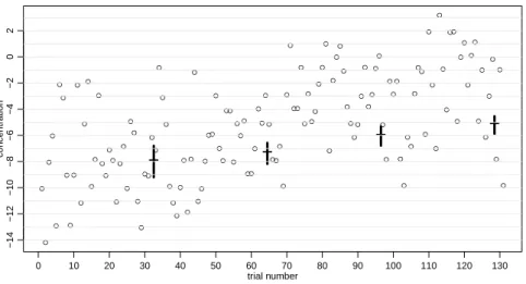
The chemist and statistician Gosset made a reality check of the fundamental assumption of independence and published the results under the pseudonym Student (1927). Between 1903 to 1926, he carefully measured the nitrogen content in pure crystalline aspartic acid once a week. This is supposedly an ideal example for the model of independent observations scattering around the true concentration. Figure 3 shows the 131 measurements from 1924 to 1926.
There appears to be an ascending and slowly oscillating trend. The confindence interval based on the whole dataset does not overlap with the one obtained for
●
●
●
●
●
●
●
●
●
●
●
●
●
●
●
●
●
●
●
●
●
●
●
●
●
●
●
●
●
●●
●
●
●
●
●
●
●
●
●
●
●
●
●
●
●
●
●●
●
●
●
●●
●
●
●
●
●●
●
●
●
●
●
●●
●
●
●
●
●●
●
●
●
●
●
●
●
●
●
●
●
●
●
●
●
●
●
●
●
●
●
●
●
●
●
●
●
●
●
●
●
●
●
●●
●
●
●
●
●
●
●
●●
●
●
●
●
●
●
●
●
●
●
●
●
●
●
0 10 20 30 40 50 60 70 80 90 100 110 120 130
−14−12−10−8−6−4−202
trial number
concentration
− − − −
Figure 3: Student’s measurements of the concentration of nitrogen in aspartic acid. The bars represent confidence intervals based on the t-test for the first 32, 64, 96,and128of 131 observations.
the first fourth of it. This indicates that the confidence intervals are too short– because independence is assumed but clearly violated.
If there is a positive auto-correlation, the variance of the mean as well as other estimators obtained from n observations is larger than the variance cal- culated under the assumption of independence. Therefore, tests and confidence intervals calculated under this assumption are liberal (true probabilities of the er- ror of the first kind are higher, intervals are too short) to an extent that depends on the auto-correlation and increases with the sample sizen.
The situation of a series of observations can be modeled by time series modelsor more generally by probabilistic process models. If an appropriate model can be found, adequate tests and confidence intervals can again be produced. In practice, auto-regressive models are often used to describe correlations between random deviations, and and they entail methods for adequate inference. Note, however, that these models assume that auto-correlations go to zero rather quickly as the lag increases. There is evidence that in reality so-called long- range dependence, describing slow decay, occurs amazingly often. Respective models are less well-known and more difficult to fit (K¨unschet al.1993).
In analogy to correlations in time, one can study correlations between close- by measurements at different locations in space. (If locations occur in groups or clusters, they lead to variance components; see Sec. 3.1.) Spatial correlations may be described and treated by the models ofspatial statistics.
3.3 Consequences for Reproducibility and Experimental Design What are the consequences of within-group, temporal or spatial correlations on reproducibility? Firstly, they often give an explanation for undesired significant differences between original and reproduced results. Secondly, if they can be adequately modeled, they may allow for a refined assessment of the validity of the original results. Specifically, if an estimate of the variance components due to “measurement campaigns” is available, it may be used to conduct a refined test of the compatibility of original and reprodued results.
The disturbing effect of correlations as mentioned above may be circum- vented or at least reduced by an adequate design of experiments. The goal of an experiment usually is to assess the effect of some “input variables” (often called
“parameters”) on a “target variable” – like the influence of a “treatment” on the yield in an industrial production. For such a goal, onlydifferences of values of the target variable are relevant.
This fact allows for avoiding disturbing effects of variance components by blocking: A block is composed of experimental units that are as homogeneous as possible with respect to nuisance factors that, while influencing the response variable, are not in the focus of the study, like measurement devices, labs, envi- ronmental conditions, subjects, time, or space.
The treatments or other variables whose effects are to be assessed should be varied within each block. Differences within a block will then be unaffected by the conditions used for blocking and lead to adequate and efficient estimates of treatment effects. Using as many blocks as possible will allow for combining these estimates and thereby gaining precision in a joint model for all blocks. We come back to these considerations in the next section. In order to allow for a soundgeneralization of results, blocks should differ in the values of the nuisance factors.
Analogous ideas can be applied to situations with temporal or spatial corre- lations. K¨unsch et al.(1993) discussed this topic in connection with long-range dependence.
If adequate blocking is used, a replication study can be conceived as the realization of more blocks, in addition to those of the original study, and a joint model may be used to check whether the new results support the original ones (see Sec. 4.2).
4 Regression Models
4.1 The Structure of Models
The vast majority of well-posed scientific questions to be studied by analyzing data lead to regression models. The variables that are observed or measured fall into three categories:
• Target variables. These variables describe the outcome, or response of a system to an input: yield, quality, population size, health indicator, survival, test score, and the like.
• Explanatory variables. They influence the target variable as inputs, or stimuli. This influence is the focus of the scientific question of the study.
Often, these variables can be manipulated in order to achieve a change in the target variable. Otherwise, there may be no causal relation, and the terms “explanatory variable” and “influence” may be misleading. In this case, the model simply describes non-causal relations.
• Nuisance variables. They also have a potential influence on the target vari- able, but their effect is not of interest and rather disturbs the examination of the influences of the explanatory variables.
Explanatory and nuisance variables will appear in the model in the same form, and we will call both of theminput variables.
A regression model describes the target variable as a function of the input variables up to random deviations. We will call its ingredients the regression functionor structural part and the error distribution or random deviations part of the model. The regression function includes parameters that are called regres- sion coefficients. The coefficients may be fixed, unknown numbers or random variables called random coefficients or random effects.
Note that all variables may be quantitative, binary, categorical or of a more involved nature. A rather comprehensive zoo of models have been developed in the last decades to cover the cases resulting from combining different types of target variables, fixed and random coefficents, kinds of functions (linear or nonlinear in the coefficients) as well as distributions and correlations of the random deviations.
As an example, consider a clinical study of a medication. The target variable may be blood pressure (quantitative), disappearance of a symptom (binary, yes or no), time to recovery (quantitative, often censored), or appearance and sever- ity of side effects (ordered categorical). The primary explanatory variable is the treatment with the medication (binary). Several other variables may be of inter- est or perceived as nuisance variables: age and gender, body mass index, fitness,
severity of disease and compliance in taking the medication. If several health care units (hospitals or physicians) are involved, they give rise to a categorical variable with random effects.
Many models combine all effects of input variables into a linear predictor, which is then related to the target variable via a link function. The linear predictor is a linear function of unknown coefficients, but need not be linear in the input variables. In fact, input variables Uk may be transformed and combined to form theterms of the linear predictorP
jβjXj(U). If only oneUk
is involved in a term (Xj =Uj or =g(Uj)), we call it a main effect, otherwise an interaction. The simplest form of an interaction term involves a product, βjkUjUk.
The structures discussed in Sec. 3.1 can be included into such a model as a random effects term, treating the grouping as a categorical variable with random coefficients. Combined with fixed effects, such models are calledmixed (effects) linear models, and a commonly used subclass are the hierarchical regression models, also called multilevel models. Correlation structures of the random deviations can also be built into regression models as a joint multivariate normal distribution with correlations given by a time series or a spatial model (Sec. 3.2).
4.2 Incorporating Reproducibility and Data Challenge
Regression models allow for prediction in a sense that refers to the idea of reproducibility: They produce a joint distribution of the values of the target variable to be obtained for given values of the input variables (those with fixed effects). Thus, they describe the expectations for the data to be obtained in a reproducibility study.
Testing the success of a reproduction for a general parameter has been introduced in Sec. 2.3 by generalizing the situation of a simple random sample in both the original and the reproduction study. In the simple case, the observations of both studies can be joined, and a toy regression model for all the data can be set up: The observations play the role of the target variable and the only explanatory variable is the binary indicator of the replication versus original study.
The test for failure of the replication is equivalent with the test for the coefficient of the study indicator to be zero.
This basic model can be enhanced with many additional features:
• Different precision of the observations in the two studies lead to a het- eroscedastic model and weighted regression for its analysis.
• Random effects and correlation terms can be incorporated to take care of the structures of variation discussed in Secs. 3.1 and 3.2.
• A random study effect can be added if an estimate for the respective variance component is available (Sec. 3.1).
• Additional explanatory and nuisance variables can be introduced. For each explanatory variable, an interaction term with the study indicator should be included to test if its effect on the target variable is different in the two studies.
The idea of a replication study leads to values of the explanatory variables that are selected to be the same as in the original study, or at least drawn from the same distribution. This is an unnecessary restriction: One could select different values for the explanatory variables on purpose and still test if themodel of the original study (including the parameters) is compatible with the new data.
Since such an approach differs from a replication study, we will refer to it by the notion of adata challenge of the model.
The notion of data challenge applies not only to regression models, but to any theory that allows for predictions of data to be expected under given circumstances. Within the context of regression, prediction is often the main goal of the modeling effort, from the development of technical processes to regression estimators in survey sampling.
It is easy to see, and well known, that predictions for values of explanatory and nuisance variables outside the range of those used for the modeling are often unreliable. Such “extrapolation” is less of a problem in our context. We will rather examine how large the differences of model coefficients between the original and the new study are – in the form of the study indicator variable and its interactions with all relevant explanatory variables – and hope that zero difference lies within the confidence intervals. Unreliable “extrapolated” predictions will be stabilized by fitting a joint model for both studies. If the new study does not incorporate similar values of explanatory variables as the original one, this adaptation may go too far, and the data challenge will not really be a challenge.
The concept of data challenge extends the notion of reproducibility in a general and useful sense: Rather than requiring new experiments or observa- tion campaigns under the same circumstances, it also allows for double-checking knowledge under different circumstances. This will often be more motivating than a simple reproduction, since it may add to the generalizability of a model.
Such studies are common in many research areas. Referrig to them as “data challenge” may express that they strengthen the reliability of models (or theo- ries).
5 Model Development and Selection Bias
5.1 Multiple Comparisons and Multiple Testing
When data are graphically displayed, our perception is typically attracted by the most extraordinary, most exceptional pattern. It is tempting to focus on such a pattern and test, with suitable procedures, if it can be produced by random variation in the data. Since our eye has selected the most salient pattern, such a test will yield significance more often than permitted by the testing level α, even if it is purely random.
In well-defined setups, such test procedures can be formalized. The simplest case is the comparison ofggroups. If we examine all pairwise differences among g= 7means by a statistical test, we will performk= 21tests. If the significance level is α = 0.05 as usual and if all observations in all groups came from the same distribution, we should expect one (wrongly) significant test among the 21that are performed. Such considerations have long been pursued and lead to appropriate tests for the largest difference of means amongg groups (and other procedures), which feature asmultiple comparisons.
In more general situations, this theme is known as multiple testing. If statistical tests onknull hypotheses are performed and all hypotheses are correct (i.e., there is no real effect at all), thefamily-wise error rateof a testing procedure is the probability that any null hypothesis is rejected. A rate bounded byα can be obtained by performing thekindividual tests at a lower level. The safest and simplest choice is the Bonferroni procedure, testing all hypotheses at the level α/k and rejecting those that turn out significant at this lower level.
These considerations formalize the concern mentioned at the beginning of this subsection, except that in an informal exploration of data it is usually unclear how many hypotheses could have caught our attention. Therefore,kis unknown.
Hence, any salient pattern should be interpreted with great caution, even if it is formally significant (at levelα). It should bereproduced with a new, independent dataset before it can be taken seriously.4
Why have we gone into lengthy arguments about the significance of tests after having dismissed their use in Section 2.4? These thoughts translate directly into conclusions about estimated effects and confidence intervals: Those that are most distant from zero will be more so than they should, and their coverage probabilities will be wrong (unless corrected adequately).
If an effect is highly significant (if zero is far from the confidence interval) and
4Collins (this volume) discusses a related issue in gravitational wave physics, where an extensive search resulted in the “detection” of spurious effects.
has a plausible interpretation, we tend to regard it as a fact without replicating it. A strict scientific rule of conduct would require, however, that an effect can only be regarded as a fact, and its precision (expressed by the confidence interval) is only reliable if derived from data that was obtained with the specific goal of testing or estimating that specific effect. Only such a setup justifies the interpretation of the testing level as the probability of an error of the first kind, or the level of a confidence interval as a coverage probability. The statistical analysis of the data obtained in such a study was calledconfirmatory analysisby John Tukey in the 1970s. But Tukey also emphasized the value of exploratory data analysis: analyzing data for unexpected patterns, with the necessary caution concerning their interpretation.
5.2 Consequences for Model Development
In many statistical studies, the relationship of one or more target variable(s) with explanatory and nuisance variables is to be examined, and the model is not fixed beforehand. Methods of model development are then used to select
• the explanatory and nuisance variables that enter the model at all,
• the functional form in which the variables enter the model (monotonic transformations, or more flexible forms like polynomials and splines, may often be adequate),
• the function that combines the effects of the resulting transformed vari- ables (non-linear, linear) and relates the combination to the target variable (via a “link function”),
• interaction terms describing the joint influence of two or more variables in a more refined way than the usual, additive form,
• any correlation structure of the random deviations if applicable.
These selections should be made with the goal of developing a model that fits the data well in the sense that there are no clear violations of the assumptions.
This relates to the exploratory mode of analysis mentioned in the preceding subsection. It would be misleading to use estimated effects, tests for a lack of effect, or confidence intervals based on such a model without any adjustments.
Developing a model that describes the data well is a task that can be as fascinating as a computer game. Strategies for doing so should be formalized and programmed. They would form procedures for the “estimation of a model” that can be evaluated. Activities in this direction have been restricted to the limited task of selecting variables from a pre-defined set of potential variables, known asmodel or variable selectionprocedures. The next task would be to formalize
the uncertainty of these procedures. In analogy to the confidence interval, one might obtain a set of models that are compatible with the data in the sense of a statistical test for the validity of a model.
Whether formalized or not, doing too good a job for this task leads to overfitting (cf. Baileyet al., this volume): The part that should remain random sneeks into the structural part. This hampers reproducibility, since the phony ingredients of the structural part of the model will be inadequate for the new study.
An alternative to developing a model along these lines is to use a very flexible class of models that adapts to data easily. Two prominent types of such classes areneural networksandvector support machines. Such model classes have been proposed mainly for the purpose of predicting the target variable on the basis of given values of the input variables. Care is needed also for these methods to avoid overfitting. The fitted models are hard to interpret in the sense of effects of the explanatory variables and therefore generally of less value for science.
An important part of model development, for which formalized procedures are available, is the task of variable selection. In order to make the problem well-defined, a sparsity condition is assumed for the correct model: Among the potential regressorsXj,j= 1, ..., p, only a subset S ={j1, j2, ..., jq} has coef- ficients βj 6= 0, and these are not too small. Thus, the true linear predictor is P
kβjkXjk. We have argued in Sec. 2.4 that such a condition is unrealistic in general, since at least tiny effects should be expected for all variables. An impor- tant field for which the condition is plausible is “omics” research: In genomics, regression models explain different concentrations of a protein by differences in the genome, and in proteomics, a disease is related to the activities of proteins.
Supposedly, only a small number of genes or proteins, respectively, influence the outcome, and the problem is to find them among the many candidates.
A model selection procedure leads to a subset S. In analogy to a clas-b sification rule, the quality of such a method is characterized by the number of regressors inSbthat are not contained inS, the “false discoveries”, and the num- ber of regressors in the true modelSthat are missed byS, the “false negatives”,b or, equivalently, the number of “true discoveries”, #(Sb∩S). The family-wise error rate introduced in Sec. 5.1 is the probability of getting at least one false discovery. A model selection procedure is consistent if it identifies the correct model with probability going to one for n → ∞. Consistent variable selection methods include methods based on the BIC criterion, the lasso and its exten- sions with suitable selection criteria, and a method introduced by Meinshausen et al.(2009), briefly characterized in Sec. 5.3. These concepts and methods are treated in depth by B¨uhlmann and van de Geer (2011).
In a reproducibility study, any variable selection procedure will most likely produce a different model. This raises the question of which aspects of the re- sults may be reproducible. Three levels may be distinguished: (a) Assuming that the procedure provides a measure of importance of the individual input variables, the more important ones should again be found in the reproduction study. A formalization of this thought seems to be lacking. (b) A less ambitious require- ment would ask for the selected model to fit the new data without a significant lack of fit. More specifically, adding variables that have been dropped by the variable selection in the original study should not improve the fit significantly (taking care of multiplicity!). (c) If the focus of the study is on prediction, a similar size of the variation of the random deviations may be enough.
An important point which is often overlooked in this context is that the effect of a variableXj on the target variabledepends crucially on the set of other variables in the model – as far as they are correlated with Xj. In (generalized) linear models, the coefficient βj of Xj measures the effect of changing variable Xj while keeping all other variables constant. Such a change may be trivial to perform or, in other applications, unrealistic or impossible, if any change of Xj leads to a change in other input variables. In fact, thescientific question must be explicit about this aspect: What should be kept constant for specifying the effect of Xj to be examined? A similar difficulty arises with interaction terms:
They imply that the effect ofXj depends on the value of another variable, and it must be clear which effect ofXj is to be estimated.
Let us use the distinction between explanatory variables, whose effects are of primary interest in the planning phase of the study, and nuisance variables, which are used to obtain a more precise model. If the nuisance variables are roughly orthogonal to (uncorrelated with) the explanatory variables, this pro- vides freedom to include or exclude the latter in the model. Thus, those having little influence on the target variable can be safely dropped. Adjustments to the inference about the explanatory variables are nevertheless necessary, as Berk et al. (2013) showed, naming the problem “post-selection inference”. The role of nuisance variables that are correlated with explanatory variables must be deter- mined without reference to the data. If a nuisance variable shows a significant, unanticipated effect, this should be interpreted with great caution.
The desired independence of the explanatory and nuisance variables can be obtained by randomization if the former can be manipulated. Thus, when the effect of a treatment is to be assessed, the assignment of individuals to the treatment or control group must be based on random numbers or on so-called orthogonal designs. The block designs mentioned in Sec. 3.3 also keep treatment and nuisance effects orthogonal.
With these rules, the effects of explanatory variables should be reproducible in the sense of Sec. 2.3, whereas inference on effects of nuisance variables is less reliable.
5.3 Internal Replication
The idea of replicating results on new data has inspired procedures which alleviate the problem of overfitting in model selection.
The choice among competing models should be based on a suitable perfor- mance measure, like a mean squared prediction error or misclassification rate. A straightforward estimation of such measures uses residuals as prediction errors or counts misclassifications of the observations of the data set used to fit the model. These estimates, however, are biased, since the estimated model fits the data better than the correct model does. In order to assess the performance correctly, a promising approach is to split the dataset into two parts, a “training set” used to estimate the model, and a “test set” for which the performance is evaluated. Clearly, this mimics an original and a replication study.
Unless the number of available observations is large, there is an obvious tradeoff when choosing the relative sizes of these two parts. A small training set leads to poor estimation of the model parameters, whereas a small test set entails an imprecise performance estimate. This tradeoff is avoided by keeping the test set small, but splitting the dataset many times, and averaging the performance estimate over all splits. The extreme choice is using a single observation as the test set. These procedures are calledcross validation.
Many model selection techniques lead, in a first step, to a sequence of models with increasing size – number of terms in a regression model. The unbiased measures of performance are used to select the final model among them.
A different approach was proposed by Meinshausenet al.(2009). They split the sample into halves, use the first part to select variables and the second to calculate a significance measure. Repeating this step for many random splits, they derive p-values for the effects of all the variables that are asymptotically correct in the sense of multiple testing and thereby get a final variable selection.
5.4 Publication and Selection Bias
The problem of multiplicity (Sec. 5.1) is also relevant for the publication of scien- tific results. Since results are hard to publish if there is no statistically significant effect (cf. Sec. 2.4), those that are published will be a selection of the studies with highest effect estimates among all conducted studies. In addition, in some
fields the effects to be examined are first selected within a study among many possible effects which can appear to be significant by choosing different target variables and exploiting the possibilities of model selection listed in Sec. 5.2.
These choices have been called “researcher degrees of freedom” (Simmons et al.2011) or “forking paths” (Gelman and Loken 2014). The published results will therefore include too high a number of “false positives”, i.e., rejections of
“correct” null hypotheses or confidence intervals excluding the zero effect value.
This was prominently discussed in the paper by Ioannidis (2005), “Why most published research findings are false”, and has lead to a considerable number of follow-up articles; see also Ehm (this volume).
Notably, the analysis by Ioannidis (2005) relies on significance testing, dis- cussed critically in Sec. 2.4, where we questioned the plausibility of an exactly zero effect. Therefore, “correct effects” would need to be defined as those that are larger than a “relevance threshold”. Then, an estimated effect would need to be significantly larger than the threshold to be regarded as a valid result. This would reduce the number of effects declared as significant, but would not rule out selection bias.
In the delicate field of drug development, the problem would lead to useless medications which by chance appeared effective in any study. This is avoided through strict regulations requiring thatclinical trials be planned in detail and announced before being carried out. Then, the decision is based on the results of that study, and no selection effect of the kind discussed above is possible. Such pre-registration has been proposed as a general remedy to fight the problem of publication and selection bias (Ioannidis 2014).
While these lines of thought consider the “correctness” of an effect obtained as significant, let us briefly discuss the consequences for reproducibility. If the effect to be tested by reproduction has been subject to selection bias in the original paper, the distribution of the estimate is no longer what has been used in Sec. 2.3, but its expected value will be smaller (in absolute value) and its variance larger than assumed. Since the biases can rarely be quantified, a success of the replication should then be defined as reaching the same conclusion, i.e. obtaining a confidence interval that again lies entirely on the same side of zero (or of the relevance threshold) as in the original study.
6 Big and High-Dimensional Data
Datasets in traditional scientific studies comprise a few dozen to several thousand observations of a few to several dozen variables. Larger datasets have appeared for a while in large databases of insurance companies and banks as well as
automated measuring instruments in the natural sciences, and the data that can be collected from the world wide web today leads into even larger orders of magnitude. If organized in rectangular data matrices, traditional modeling treats clients, time points and records as “observations”, and their characteristics, concentrations of substances and fields in records as “variables”.
Usually, the number of observations grows much more rapidly than the num- ber of variables, leading to the problem of handlingbig data. The large number of observations allows for fitting extremely complicated models, and it is to be expected that no simple model fits exactly, in the sense of showing non-significant results for goodness-of-fit tests. Nevertheless, it is often more useful to aim for simple models that describe approximate relationships between variables. Other typical problems deal with searching patterns, like outliers hinting to possible fraud or other extraordinary behavior, or clusters to obtain groups of clients to be treated in the same way (see Estivill-Castro, this volume).
A useful strategy to develop reasonable models for big data is to start with a limited random subset, for which traditional methods can be used, and then validate and refine them using further, larger subsets. In principle, all aspects of reproducibility checks can then easily be applied within the same source of data, possibly for studying its stability over time. However, when descriptive methods are applied that do not intend to fit a parametric model (as is typical for cluster analysis), it may be unclear how the results of their application to subsets or different studies should be compared.
In genomics and proteomics, the situation is reversed as compared to “big data”: Measurements of thousnads of “variables” are collected on chips, which are used on a few dozen or a few hundred subjects. This leads tohigh-dimensional data. In this situation, traditional methods typically fail. Regression models can- not be fit by the popular least-squares principle if the number of observations is smaller than the number of coefficients to be estimated. The basic problem here is variable selection, for which reproducibility has a special twist, as discussed in Sec. 5.2.
7 Bayesian Statistics
In the introduction, the core business of statistics was presented as providing a way to quantitatively express uncertainty, and confidence intervals were pro- posed as the tools of choice. Another intuitive way to describe uncertainty is by probabilities. The parameter to be assessed is then perceived as a random variable whose distribution expresses the uncertainty, and it does so in a much more comprehensive way than a simple confidence interval does.
This is the paradigm underlying Bayesian statistics, where the distribution of the parameter expresses the belief about its plausible values. This allows for formalizing, by theprior distribution, what a scientist believes (knows) about a parameter before obtaining data from which to draw inferences about it. When data becomes available, the belief is updated and expressed again as a distribu- tion of the parameter, called theposterior distribution.
The general rule by which updating is performed is the formula of Bayes connecting conditional probabilities – whence the name of the paradigm. The idea of Bayesian statistics is to describe in a rational way the process oflearning from a study or, by repeated application, from a sequence of studies. Note that the idea still is that there is a “true value” of the parameter, which would even- tually be found if one could observe an infinite amount of data. The distribution of the parameter describes the available knowledge about it and hopefully will have a high density for the true value.
It is useful to distinguish the two kinds of probabilities involved:
• The prior distribution expresses a belief and is, as such, not objective.
It may be purely subjective or based on the consent of experts. Such probabilities describe epistemic.knowledge and their use contradicts the objective status of a science which is supposed to describe nature. This is not too severe if we accept that objectivity in this sense is an idealization which cannot be practically achieved.
Furthermore, if little is knowna priori, this may be expressed as a “flat” or
“uninformative” prior distribution. This leads us back to an analysis that does not depend on a subjective choice of a prior distribution.
• The probability model that describes the distribution of the observations for given values of the parameters is of a different nature. The correspond- ing probabilities are calledfrequentistor aleatory. This is the model used in the main body of this paper. Note that the choice of the model often includes subjective elements and cannot be reproduced “objectively”, as discussed in Sec. 5.
The paradigm of Bayesian statistics is in some way contrary to the idea of reproducibility, since it describes the process of learning from data. For a replication study, the posterior distribution resulting from the original work would be used as a prior, and the new data would lead to a new, sharper posterior distribution of the parameter.
On the other hand, judgments about the success of a replication attempt can be formalized by quantifying the evidence from the new data for the hypotheses of a zero and of a nonzero effect. When a prior distribution for the effect parameter is fixed, the (integrated) likelihood can be calculated for the nonzero
effect hypothesis, and compared to the likelihood under the null hypothesis. The ratio of the two likelihoods is called theBayes factor.
Verhagen and Wagenmakers (2014) explain this idea and propose, in the replication context, to use the posterior distribution of the original study as the prior within the non-zero hypothesis for this evaluation. This leads to a
“point estimate” for the Bayes factor and leaves the judgement whether the evidence expressed by it should suggest a success or a failure of replication open. Reasonable boundaries for such a decision would depend on the amount of information in the data of the original and the replication studies (and in the prior of the original study, which may be standardized to be non-informative).
Gelman (2014) advocates the use of Bayesian statistics as an alternative to hypothesis testing, cf. Sec. 2.4. On the one hand, he suggests to boost the insufficient precision of studies with small sample sizes by using an informative prior distribution. We strongly prefer to keep the information expressing prior knowledge separated from the information coming from the data for the sake of transparency, especially for readers less familiar with the Bayesian machinery.
On the other hand, Gelman advocates the use of multilevel models, which are often formulated in Bayesian style. We agree with this recommendation, but prefer the frequentist approach as described in Sec. 3.1.
8 Conclusions
8.1 Successful Replication
Reproducibility requires that a scientific study should be amenable to replication and, if performed again, should yield “the same” results within some accuracy.
Since data is usually subject to randomness, statistical considerations are needed.
Probability models are suitable to distinguish between a structural part that should remain the same for the replication study, and random deviations that will be different, but still subject to a supposed probability distribution.
Clearly, this is an idealized paradigm. It relies on the assumption that the
“circumstances” of the new study are “the same” in some sense of stability (cf. Tetens and Steinle, both in this volume). Stochastic models may include components to characterize the extent of such stability in a realistic manner:
Usually, a variance component that describes the deviations from experiment to experiment or period to period will be appropriate. The lack of such a component may be a candidate to explain the common experience that reproducibility fails too often.
One can formalize a successful replication as one for which the difference
from the original study in the estimate of the parameter of interest θ is not significantly different from zero. This may lead to different situations for the conclusion about the effect measured by θ itself. As an extreme example, one might have a significantly positive estimate θbin the original study and a (non- significant) negative estimate in the replication, and still get an insignificant difference so that the replication would look successful. Thus, it is useful to distinguish two aspects:
• Statistical compatibility: Is the data obtained in the replication compatible with the data from the original study in the light of the model used to draw inference? If not, this may point to a flaw in the model, like neglecting a source of variability, to a selection bias, to manipulation of data, or to a failure to reproduce the same circumstances.
• Confirmation of conclusions: Does the replication study lead to the same conclusions as the original one? If a relevant effect has been found in the original study, one would hope to find it again (as statistically signif- icant) in the replication. The result may then be indecisive, if statistical compatibility is fulfilled, but significance fails in the repeated study.
8.2 Validation and Generalization
In designing studies for empirical modeling, there is a tradeoff between keeping the circumstances as homogeneous as possible to get clearly interpretable results and making them as different as possible to get generalizability, i.e., to allow for more generally applicable conclusions. The latter suggests to repeat an experiment under different conditions, as discussed above, using block designs (Sec. 3.3), or including nuisance variables that characterize different conditions.
This may also suggest anextension of the notion of reproducibility to include studies that explore different circumstances with the expectation to reproduce the essentialconclusionsfrom an original study rather than reproducing the data. We introduced the concept ofdata challengefor such studies (Sec. 4.2). However, it is not clear if possible discrepancies should be interpreted as a failed replication or as a variation due to altered circumstances. A most rewarding way to conduct validation studies will be to design a replication part geared at reproducing the results under the same circumstances and an additionalgeneralization part, varying them to yield the potential for novel insight.
Another, related direction of extending the idea of reproducibility is thecon- ceptual replication, in which the essential conclusions of a study are examined, intentionally using different methods than in the original study. In psychology, the personality characteristics, called “traits” or “constructs”, cannot be mea- sured directly, but are derived from the analysis of questionnaire data or from