On the Interplay between Keynesian and Supply Side Economics

IHS Economics Series Working Paper 206

April 2007

On the Interplay between Keynesian and Supply Side Economics

Marika Karanassou

Impressum Author(s):

Marika Karanassou, Dennis J. Snower Title:

On the Interplay between Keynesian and Supply Side Economics ISSN: Unspecified

2007 Institut für Höhere Studien - Institute for Advanced Studies (IHS) Josefstädter Straße 39, A-1080 Wien

E-Mail: o ce@ihs.ac.atffi Web: ww w .ihs.ac. a t

All IHS Working Papers are available online: http://irihs. ihs. ac.at/view/ihs_series/

This paper is available for download without charge at:

https://irihs.ihs.ac.at/id/eprint/1767/

206 Reihe Ökonomie Economics Series

On the Interplay between

Keynesian and Supply Side

Economics

206 Reihe Ökonomie Economics Series

On the Interplay between Keynesian and Supply Side Economics

Marika Karanassou, Dennis J. Snower

April 2007

Contact:

Marika Karanassou Department of Economics Queen Mary and Westfield College Mile End Road

London E1 4NS, United Kingdom email: m.karanassou@qmul.ac.uk Dennis J. Snower

The Kiel Institute for the World Economy Düsternbrooker Weg 120

24105 Kiel, Germany : +49/431/8814-235

email: dennis.snower@ifw-kiel.de

Founded in 1963 by two prominent Austrians living in exile – the sociologist Paul F. Lazarsfeld and the economist Oskar Morgenstern – with the financial support from the Ford Foundation, the Austrian Federal Ministry of Education and the City of Vienna, the Institute for Advanced Studies (IHS) is the first institution for postgraduate education and research in economics and the social sciences in Austria.

The Economics Series presents research done at the Department of Economics and Finance and aims to share “work in progress” in a timely way before formal publication. As usual, authors bear full responsibility for the content of their contributions.

Das Institut für Höhere Studien (IHS) wurde im Jahr 1963 von zwei prominenten Exilösterreichern – dem Soziologen Paul F. Lazarsfeld und dem Ökonomen Oskar Morgenstern – mit Hilfe der Ford- Stiftung, des Österreichischen Bundesministeriums für Unterricht und der Stadt Wien gegründet und ist somit die erste nachuniversitäre Lehr- und Forschungsstätte für die Sozial- und Wirtschafts- wissenschaften in Österreich. Die Reihe Ökonomie bietet Einblick in die Forschungsarbeit der Abteilung für Ökonomie und Finanzwirtschaft und verfolgt das Ziel, abteilungsinterne Diskussionsbeiträge einer breiteren fachinternen Öffentlichkeit zugänglich zu machen. Die inhaltliche Verantwortung für die veröffentlichten Beiträge liegt bei den Autoren und Autorinnen.

Abstract

Conventional wisdom suggests that nominal, demand-side shocks have only temporary effects on real macroeconomic magnitudes and that the duration of their effects depends on the degree of nominal inertia. It is also argued that, in the absence of unit roots, temporary supply-side shocks also have only temporary real affects and that the duration of these effects depends on the various sources of real inertia. Our analysis indicates that there is a potentially important interplay between real and nominal inertia in generating the persistent effects of real and nominal shocks. In this sense, then, Keynesian and supply-side economics are mutually interdependent. Our analysis has identified circumstances when real and nominal inertia are complementary in generating real and nominal persistence. Here, we argue, lies a potentially crucial, but as yet largely unexplored, set of determinants of the effectiveness of Keynesian and supply-side economic policies.

Keywords

Unemployment, employment, wage setting, labour force participation, labour market

dynamics, unemployment persistence, imperfect unemployment responsiveness

Comments

We gratefully acknowledge the funding of this research by a grant of the Jubilaeumsfonds of the Austrian National Bank (Project No. 10088).

Contents

1 Introduction 1 2 A Simple Model of Nominal Persistence 4

2.1 Structure of the Model ... 5

2.2 Nominal Persistence ... 6

2.3 The Relation between Persistence and Inertia ... 7

2.4 Some Intuition ... 9

3 Extensions 11

3.2 Market-Clearing Prices ... 13

3.3 Keynesian Transmission of Nominal Shocks ... 14

4 Concluding Thoughts 15

References 16

Figures 18

1 Introduction

There is a vast macroeconomic literature indicating that the effectiveness of Keynesian demand-side policies depends primarily on the degree of nominal inertia (how long it takes for nominal wages and prices to adjust to shocks);

and there is another large literature on hysteresis and unemployment per- sistence which indicates that the impact of temporary supply-side shocks depends primarily on the degree of real inertia (how long it takes for real variables, such as output and employment, to adjust to shocks). This paper is concerned with the dynamic interplay between these two types of inertia and the resulting interaction between Keynesian and supply-side economics.

The nominal inertia in the Keynesian models can arise from various sources, such as costs of wage-price adjustment, near-rationality, or wage- price staggering.

A well-known result in this literature is that nominal, demand-side shocks (such as money supply shocks) have only temporary ef- fects on output and employment, and that the degree of nominal persistence - the degree to which the output-employment effects of nominal shocks persist through time - depends on the degree of nominal inertia.

In the literature on hysteresis and unemployment persistence, the real inertia can arise from various sources, such as employment adjustment costs

(such as costs of hiring and firing labour, so that current employment depends on past employment), insider membership effects

(so that the current real wage depends on the size of the insider workforce, which depends on past employment), and discouraged long-term unemployed effects

(so that search intensity falls with unemployment duration and consequently the current real wage depends on past unemployment). In this literature, temporary productivity shocks can have persistent effects on output, employment, and unemployment, and the degree of real persistence - the degree to which the output-employment effects of temporary real shocks persist through time - depends on the magnitude of real inertia.

Out of these two strands of literature has grown the conventional macroe- conomic wisdom that links nominal persistence to nominal inertia, and links real persistence to real inertia. This view - which we call the persistence-

1See, for example, Akerlof and Yellen (1985), Blanchard (1986), Mankiw (1985), and Taylor (1979, 1980).

2This view has found its way into most economic textbooks (e.g. Mankiw (1997); it originated from the quantity rationing macro literature (e.g. Barro and Grossman (1976), Malinvaud (1977)).

3For example, Nickell (1978).

4For example, Blanchard and Summers (1986) and Lindbeck and Snower (1987).

5For example, Bean and Layard (1988).

inertia correspondence - is pervasive. For instance nominal rigidities play a prominent role in the analysis of the real effects of monetary policy, while real rigidities are dominant in explanations of why European unemployment responds slowly to macroeconomic fluctuations.

The purpose of this paper is to call this conventional macroeconomic wis- dom into question. We show that the output-employment effects of nominal demand shocks do not just depend on nominal inertia, and similarly the real effects of temporary supply-side shocks do not just depend on real inertia.

On the contrary, real inertia can play a powerful role in propagating the real effects of nominal, demand-side shocks through time, and nominal inertia may be important in propagating the real effects of real, supply-side shocks.

We make this point as transparently and powerfully as possible by con- structing a sequence of simple, illustrative macroeconomic models that high- light the influence of real and nominal inertia on real and nominal persistence.

Our aim is to show how the persistent output-employment effects of real and nominal shocks arise from the interaction between the sluggish wage-price adjustment and sluggish output-employment adjustment. In the process, we indicate that nominal inertia does not necessarily have a dominant influence on nominal persistence, nor does real inertia necessarily have a dominant influence on real persistence. Furthermore, the relative magnitudes of real and nominal persistence depends on the interplay between real and nominal inertia.

Our analysis has potentially important implications for macroeconomic policy. First, by showing that the real effects of monetary policy depend on the interplay between real and nominal inertia, our analysis implies that the standard Keynesian theory of monetary policy in terms of nominal rigidities is seriously incomplete. Second, since the real effects of temporary supply- side policy changes (such as temporary investment tax credits, recruitment subsidies, and education and training grants) likewise depend on the interac- tion between the two forms of inertia, our analysis suggests that the policy implication of the New Classical Macroeconomics, the Real Business Cycle school, and the hysteresis theory - all of which tend to overlook the implica- tions of nominal rigidities - also are too narrowly focused. Third, supply-side policies that reduce real inertia are often complementary to those that reduce nominal inertia, in the sense that the combined effect of these policies on real and nominal persistence is greater than the sum of the individual effects. For example, a relaxation of job security provisions that reduces employment ad- justment costs (and thus makes current employment less dependent on past employment) is complementary to a collective bargaining reform that re- duces wage adjustment costs (and thus makes the current nominal wage less dependent on the past nominal wage).

2

Although the existing literature on slow adjustment of real and nominal variables often uses the terms “rigidity,” “stickiness,” “sluggishness,” and

“inertia” interchangeably, it is vital for our purposes to make a sharp dis- tinction between the following economic phenomena. The first is absolute inflexibility, perhaps best described by the term “rigidity,” so that for in- stance “price rigidity” means that prices do not move at all in response to shocks. The literature on menu costs is about this phenomenon (i.e. on ac- count of the costs of price change, firms may find it profitable to hold prices constant in the presence of changes in demand).

The second phenomenon is slow adjustment, which we call “inertia,” so that for instance “price inertia” means that prices do not respond fully to clear their respective markets within a given period of time. The literature on unemployment persistence deals with this phenomenon (e.g. if employment and real wages adjust slowly to productivity shocks, it takes a long time before unemployment reaches its long-run equilibrium).

And the third phenomenon concerns a comparative static unresponsive- ness ; for example, in the macroeconomic literature “real wage rigidity” often means that the labour demand and labour supply curves are flat (in real wage-employment space), so that if either of these curves shifts, the equi- librium real wage does not move much. Much of the literature on the joint swings in employment and wage-price mark-ups

concerns this phenomenon (e.g. if the labour demand curve is flat, then intertemporal substitution of leisure for labour will lead to large employment changes relative to the real wage changes).

In this paper we concentrate attention exclusively on the second phe- nomenon, “inertia.” A large body of empirical evidence suggests that this phenomenon is of pervasive importance. For example, a common finding in the empirical literature on New Keynesian economics is that many firms change their prices frequently but not by sufficient amounts to operate the need for large quantity adjustments.

This result is suggestive of price in- ertia. In the same vein, the empirical literature on labour demand suggests that employment responds slowly to productivity shocks. This paper will an- alyze how the interaction between real and nominal inertia gives rise to real and nominal persistence, and will thereby elucidate the interdependence of demand-side and supply-side mechanisms in generating business fluctuations.

Surprisingly, this issue of potentially far-reaching importance has not, to the best of our knowledge, been explored explicitly in the macroeconomic

6See, for example, Bils (1987), Hall (1986), McDonald and Solow (1981), Rotemberg and Saloner (1986), and Stiglitz (1984).

7See, for example, Carlton (1986).

literature thus far. Although it has become well-known that “real rigidities”

reinforce “nominal rigidities” in making monetary shocks non-neutral, the

“rigidities” considered in the existing literature do not refer to inertia. This significant point is obscured by the usual practice of using the term “rigidity”

to refer to all three of the phenomena above. For example, in Ball and Romer (1990), “nominal rigidity” refers to the first phenomenon (menu costs) and “real rigidity” refers to the third (small responsiveness of equilibrium relative prices to changes in real money balances); whereas in Blanchard (1987), “nominal rigidity” refers to the second phenomenon (slow adjustment of nominal wages to prices and vice versa) while “real rigidity” refers to the third (slow response of mark-ups to output and employment). Clearly, there is a world of a difference between the statement (a) that a comparative static unresponsiveness augments an absolute price inflexibility (as in Ball and Romer), (b) that a comparative static unresponsiveness augments the slow adjustment of prices through time (as in Blanchard), and (c) that real and nominal inertia interact in determining the price-quantity effects of real and nominal shocks (as in this paper).

This paper is organised as follows. Section 2 presents a particularly sim- ple macroeconomic model that brings the interplay between real and nominal inertia into sharp relief. In this context we derive measures of real and nom- inal persistence and examine how these measures are related to real and nominal inertia. then the relation between persistence and inertia. Section 3 generalises this model in straightforward ways to clarify some further signif- icant channels whereby real and nominal inertia generate real and nominal persistence. Finally, Section 4 concludes.

2 A Simple Model of Nominal Persistence

The following macroeconomic model provides a particularly straightforward vehicle for examining the relation between persistence and inertia. The model focuses on nominal persistence. Specifically, it illustrates how nominal per- sistence arises from the interaction between real and nominal inertia. For simplicity, the model allows nominal shocks to have lagged effects on both prices and quantities; but, for analytical and conceptual simplicity, we allow real shocks to influence only quantities (not prices). Thus the model is able to illustrate simply how nominal persistence arises from the interaction between real and nominal inertia, but real persistence depends only on real inertia.

Subsequent sections then extends this model to show how the interaction be- tween real and nominal inertia can generate real persistence and allow for a richer set of channels whereby demand- and supply-side mechanisms interact.

4

2.1 Structure of the Model

In our model real inertia takes a simple form: current employment depends on past employment, say, on account of firms’ employment adjustment costs

. Specifically, let E

be aggregate employment, K

be the aggregate capital stock, W

be the nominal wage, and P

be the price level. (All variables are in logs.) Then the aggregate employment

is given by

E

= a + a

E

− a

(W

− P

) + a

K

+ ε

, (1) where a, a

, a

are positive constants, 0 < a

< 1, and ε

∼ i.i.d (0, σ

), representing the temporary real shock. The coefficient a

may be called the

“real inertia coefficient.”

Let the aggregate production function be

Q

= β

+ β

E

(2)

where Q

is aggregate output and β

and β

are positive constants.

The nominal inertia in the model also takes a simple form: the current nominal wage depends on the past nominal wage, as in wage staggering models. Specifically, the nominal wage is taken to depend on its past value and the money supply M

:

W

= b

W

+ (1 − b

) M

+ e

, (3) where 0 < b

< 1, and e

∼ i.i.d (0, σ

).

This wage determination mech- anism is a variant of the model of Taylor (1979), and the coefficient b

may accordingly be called the “nominal inertia coefficient.”

To keep the model transparent, we assume that the price level responds instantaneously to the money supply, as follows:

P

= M

+ e

, (4)

where e

∼ i.i.d (0, σ

) . Finally, the money supply is subject to permanent shocks:

M

= M

+ µ

, (5)

8See, for example, Nickell (1978). These costs may take the form of hiring, training, and firing costs.

9In a standard macro model, the corresponding level of output could be given by an aggregate production function, such asQt=β₀+β₁Et.But since output plays no role in our subsequent analysis, we ignore this function here.

10The coefficients of W_t−1 and of Mt must sum to unity in order to ensure money neutrality in the long run.

where µ

∼ i.i.d 0, σ

. We assume that the error terms ε

and µ

are in- dependent of each other, so that a monetary shock has no direct effect on employment. Observe that since the coefficients of W

and of M

sum to unity, money is neutral in the long run (

=

= 1); and thus monetary shocks have only temporary effects on employment.

The macroeconomic equilibrium in any period t is given by the solution of the system (1)-(4). Observe that by (3)-(5), the real wage is W

− P

= b

(W

− P

) − b

∆M

+ e

, so that

W

− P

= −b

µ

+ e

1 − b

B , (6)

where e

= e

− (1 − b

B) e

, and B is the backshift operator. Substituting (6) into (1), we find that employment is described by the following dynamic process:

E

= (a

+ b

) E

− a

b

E

+ a

b

µ

+ ζ

, (7) where ζ

= −a

e

+ (1 − b

B) (a + a

K

+ ε

). Normalising β

= 1 in equation (2), the solution to (7) implies the following equilibrium time path for aggregate output:

Q

=

a

− b

a

− b

(a

b

µ

+ ζ

) +

a

− b

a

− b

a

b

µ

+ ζ

+

a

− b

a

− b

a

b

µ

+ ζ

+ ... (8)

In this context we now derive our measure for nominal persistence.

2.2 Nominal Persistence

“Nominal persistence” arises when the monetary shock µ

has long-lasting effects on aggregate output, i.e. the shock µ

influences output beyond period t. A straightforward way of measuring the degree of nominal persistence is in terms of the sum of the differences between output in the presence and absence of the shock, from period t onwards.

Specifically, consider a one-off unit monetary shock dµ

= 1 (dµ

= 0, j > 0) and let d

Q

be the resulting difference between period-t+j output in the presence of the shock Q

and in the absence of the shock (Q

):

d

Q

= Q

− Q

, j ≥ 0, where the superscript (N ) indicates that the difference in outputs is generated by a “nominal” shock. Summing over all

11See Appendix 1.

6

periods subsequent to the shock (j > 0), we obtain our measure of nominal persistence:

π

=

∞

X

j=1

d

Q

. (9a)

By (8) and (9), it can be shown that the degree of nominal persistence in our model is

π

= b

a

(a

+ b

− a

b

)

(1 − a

) (1 − b

) . (9b) We are now in a position to examine the interplay between real and nominal inertia in generating nominal persistence.

2.3 The Relation between Persistence and Inertia

The relation between persistence and inertia in our model may be summarised by the following propositions.

Proposition 1: Nominal inertia is a necessary condition for nominal persistence.

In the absence of nominal inertia, b

= 0, and then, by equation (9b), there is no nominal persistence: π

= 0. Intuitively, if there is no nominal inertia, a nominal shock (µ

) has the same effect on the nominal wage (W

) as on the nominal price level (P

), and thus leaves the real wage (W

− P

) unchanged. Consequently, the money shock has no output effects, so that there is no nominal persistence.

Proposition 2: The relative magnitude of nominal and real persistence does not depend simply on the relative magnitude of nominal and real iner- tia. Rather, the output effects of real versus nominal shocks depend on the interplay between nominal and real inertia.

From equations (9b) and (9b), we find that

π

Q π

⇔ a

Q a

(1 − b

)

b

[a

(1 − b

) + b

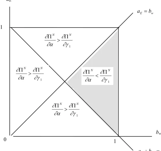
] (10) Figure 1 illustrates the relation between nominal and real persistence by picturing π

= π

in terms of the real wage elasticity of labour demand a

and the inertia coefficients a

and b

. For values of b

that lie above this surface, π

> π

; and for b

below the surface, π

< π

. The figure indicates a range of values for which

12The implications of this equation for the parameter values are given in Appendix 1.

• real persistence exceeds nominal persistence (b

lies above the surface π

= π

, so that π

< π

) even though real inertia is less than nominal inertia (a

< b

) , and

• nominal persistence exceeds real persistence (b

lies below the surface π

= π

, so that π

> π

) even though nominal inertia is less than real inertia (b

< a

).

To gain insight into Figure 1, it is useful to observe that

nominal inertia affects nominal, but not real, persistence. Thus, as the degree of nominal inertia rises, nominal persistence rises relative to real per- sistence.

• By contrast, real inertia affects both nominal and real persistence. The relative magnitude of these effects depends on the degree of nominal inertia (due to the complementarity between real and nominal inertia, described in Proposition 4 below).

• Specifically, for low values of b

, i.e

W

> a

, real inertia has a stronger effect on real persistence than on nominal persistence:

E

>

∂π^N

∂aE

. Then, in order for the difference between real and nominal persis- tence to remain the same, a rise in nominal inertia (b

) must be met by a rise in real inertia (a

). But for high values of b

, i.e

W

< a

, real inertia has a stronger effect on nominal persistence. Then, a rise in nominal inertia must be met by a fall in real inertia so that the initial difference between real and nominal persistence to remain unchanged.

In this way, Figure 1 provides a clear illustration of the interaction be- tween real and nominal inertia in generating nominal persistence.

Proposition 3: Nominal inertia does not necessarily have a greater influ- ence than real inertia on the degree of nominal persistence.

From equations (9a and 9b) it is clear that when b

> 0, the degree of nominal persistence π

does not depend solely on the nominal inertia coefficient b

, but also on the real real inertia coefficient a

. Specifically, from (9), we find

that nominal inertia has a positive effect on nominal persistence:

∂π

∂b

= a

b

(1 − a

) (1 − b

)

+ a

+ b

(1 − a

) (1 − a

) (1 − b

)

> 0, (11a)

13See Appendix 1

8

and real rigidities also have a positive effect:

∂π

∂a

= a

b

(1 − a

)

(1 − b

) > 0, (11b) since a

, b

> 0.

The sign of

∂bW

−

E

depends on the inertia coefficients a

and b

. Observe that nominal inertia does not necessarily have a greater influence than real inertia on the degree of nominal persistence. Rather, when nominal inertia is smaller than real inertia and as the sum of the two exceeds unity, then the effect of real inertia on nominal persistence comes to dominate the effect of nominal inertia on nominal persistence.

Proposition 4: Nominal inertia does not necessarily have a greater influ- ence than real inertia on the degree of nominal persistence.

From equations (9a and 9b) we find that the greater is the degree of real inertia, the stronger will be the effect of nominal inertia on nominal persistence (and, conversely, the greater the degree of nominal inertia, the stronger is the effect of real inertia on nominal persistence):

∂

π

∂b

∂a

= a

(1 − a

)

(1 − b

)

> 0, (12) Thus the joint effect of nominal and real inertia on nominal persistence is stronger than the sum of the individual effects.

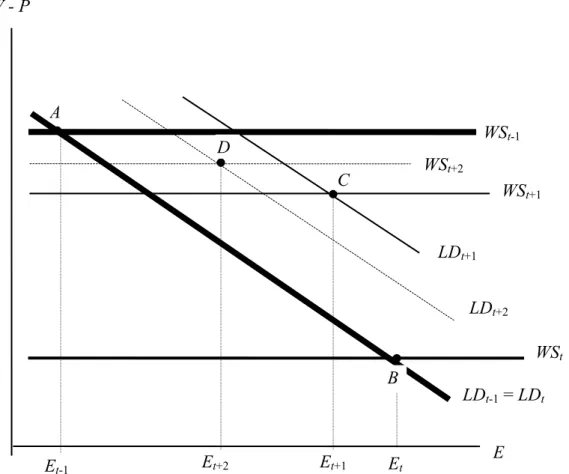
2.4 Some Intuition

Figure 3 helps provide an intuitive understanding of how real and nomi- nal inertia interact to generate nominal persistence. The initial, stationary labour market equilibrium (in period t − 1) is depicted by point A, at the intersection between the labour demand curve LD

and the wage setting curve W S

. Thereupon a positive nominal shock (µ

) occurs in period t.

Since wage movements in our model are characterised by inertia whereas price movements are not (by equations (3) and (4)), the nominal shock has a stronger effect on the price level than on the wage, so that the real wage (W

− P

) falls.

Thus the wage setting curve shifts down from W S

to W S

in the figure. The associated labour market equilibrium shifts from Point A to B, and employment rises from E

to E

.

In the following period t + 1, the nominal shock has disappeared, but nominal wage inertia prevents the wage setting curve from returning imme- diately to its initial position (W S

): since the real wage (W

− P

) is below

14Observe that in equation (6) the nominal shockµ_tis inversely related to (W_t−P_t).

its initial value, nominal wage inertia implies that the wage setting curve W S

lies beneath its initial position. In the same vein, since employment E

is above its initial value, real inertia implies that the labour demand curve LD

rises above its initial position. Consequently, the labour market equilibrium shifts from Point B to C.

In period t + 2, the wage setting curve shifts upward, as nominal inertia reflects the wage increase of period t + 1 (associated with the move from Point B to C). Furthermore, real inertia ensures the period t + 1 fall in employment (also associated with the move from B to C) shifts the period t + 2 labour demand curve downwards. Consequently, the labour market equilibrium shifts from Point C to D in period t + 2. And along the same lines, this equilibrium thereafter gradually approaches the initial equilibrium at Point A.

Note that in the absence of nominal inertia (b

= 0), the money supply has no effect on the real wage (by equations (2) and (3)), and since the real wage is the only channel whereby monetary shocks can affect employment in our model, these shocks cannot generate nominal persistence (as stated in Proposition 1).

Furthermore, observe the interdependent roles of nominal and real inertia in generating nominal persistence. On account of nominal inertia (b

> 0), the wage setting curve returns to its initial position only gradually; and on account of real inertia (a

> 0), the labour demand curve does so as well.

Both types of inertia not only contribute positively to nominal persistence, they are complementary to one another (as stated in Proposition 4). The reason is straightforward: (a) the greater the degree of nominal inertia, the more slowly the wage setting curve approaches its initial equilibrium; (b) consequently, the more slowly the level of employment approaches its initial equilibrium; and, on account of real inertia, (c) the more slowly the labour demand curve approaches its initial equilibrium. In this way, real inertia gives greater leverage to the influence of nominal inertia on nominal persistence.

On account of this complementarity between nominal and real inertia in generating nominal persistence, it follows that the relative magnitudes of nominal and real persistence must depend on the interplay between nom- inal and real inertia (as stated in Proposition 2). Finally, since the effect of nominal (real) inertia on nominal persistence depends on real (nominal) inertia, it is not surprising that nominal inertia does not necessarily have a bigger influence on nominal persistence than does real inertia (as stated in Proposition 3).

10

3 Extensions

The model of the previous section is clearly restrictive in the following re- spects: (a) nominal inertia has no influence on real persistence (although real inertia does affect nominal persistence), (b) the price equation has an extremely simple form, which does not ensure that the price level clears the product market; (c) nominal inertia pertains solely to wages, so that there is no consideration of how price inertia opens up Keynesian channels whereby nominal shocks may be transmitted to employment and production. In this section we generalise the model to remove these restrictions.

3.1 Nominal Inertia and Real Persistence

A simple, plausible way of allowing both nominal and real inertia to influence nominal and real persistence is to extend the wage equation to take account of the influence of employment on wage determination. Then nominal shocks can affect real variables via the effect of the real wage on employment, and real shocks can affect nominal variables via the effect of employment on the nominal wage. In line with the bulk of the prevailing evidence, we assume that, given the size of the labour force and the price level, the greater is the level of employment, the greater will be the nominal wage (ceteris paribus).

Thus the wage equation becomes

W

= b

W

+ (1 − b

) M

+ b

E

+ e

, (13) where b

is a positive constant.

Incorporating this wage equation into the previous model, we obtain

the following expressions for nominal and real persistence

π

=

b

a

1 + b

a

a

+ b

− a

b

(1 − a

) (1 − b

) + b

a

, (14a)

π

=

1 1 + b

a

a

− a

b

− b

b

a

(1 − a

) (1 − b

) + b

a

. (14b)

#

It is straightforward to show

that Propositions 1-4 continue to hold in this extended model. In addition, we can now analyze the influence of both real and nominal inertia on the degree of real persistence:

15See Appendix 2.

16See Appendix 2.

Proposition 5: Real inertia is a necessary condition for positive real per- sistence; but negative real persistence is possible even in the absence of real inertia.

By equation (14b), in the absence of real inertia (a

= 0), the degree of real persistence is

π

= −

1 1 + b

a

b

b

a

1 − b

+ b

a

< 0. (14b’) Proposition 6: The degree of real persistence depends on the degree of both real and nominal inertia. Real persistence rises in response to an increase in real inertia, but falls in response to an increase in nominal inertia.

By equation (14b), the degree of real persistence π

depends on both the real inertia coefficient a

and the nominal inertia coefficient b

:

∂π

∂a

= (1 − b

)

[(1 − a

) (1 − b

) + b

a

]

> 0, (15a)

∂π

∂b

= −a

b

[(1 − a

) (1 − b

) + b

a

]

< 0. (15b) Proposition 7: The magnitude of real persistence depends on the interac- tion between real and nominal inertia.

By equation (14b), we obtain:

∂

π

∂b

∂a

= −2a

b

(1 − b

)

[(1 − a

) (1 − b

) + b

a

]

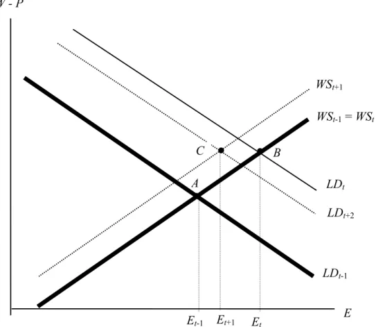
< 0. (16) Figure 3 illustrates the intuitive rationale underlying Propositions 5-7. A positive real shock in period t (ε

) shifts the labour demand curve outward from LD

to LD

along the wage setting curve W S

(= W S

). Thus the labour market equilibrium moves from Point A to B , and the real wage (W

− P

) and employment E

both rise above their initial equilibrium values.

In the following period t + 1, the real shock has disappeared, but the real inertia implies that the labour demand curve moves only partially towards its initial position. Furthermore, the nominal inertia implies that the wage setting curve rises above its initial position. Consequently the labour market equilibrium moves from Point B to C. Thereafter the labour demand and wage setting curves gradually return to their initial positions, so that the labour market equilibrium returns to Point A in the long run.

The figure indicates why real and nominal inertia exert opposing influ- ences on real persistence (in contrast to their effect on nominal persistence).

The greater the degree of real persistence, the longer the labour demand

12

curve remains above its initial position, and thus the more prolonged will be the positive employment effect of a temporarily real shock. However, the greater the degree of nominal persistence, the longer the wage setting curve remains above its initial position, and this dampens the employment effect of the real shock.

Furthermore, observe that in the absence of real inertia, the labour de- mand curve returns to its initial position as soon as the real shock disappears.

But in the presence of nominal inertia, the wage setting curve remains above its initial position for a prolonged span of time. The resulting persistence is negative.

3.2 Market-Clearing Prices

We now allow for a price level that clears the product market. For simplic- ity, suppose that product demand is proportionately related to real money balances so that, in logs,

Q

= d

+ (M

− P

) +

, (17a) where d

is a constant and

is strict white noise. Furthermore, suppose that product supply depends on employment via a Cobb-Douglas production function so that, in logs,

Q

= d

+ d

E

+

, (17b) where d

, d

are constants, d

> 0, and

is strict white noise. Thus the price level clears the product market Q

= Q

when

P

= d

− d

+ M

− d

E

+

, (18) where

=

−

.

Substituting the price equation (21) for (3) in our model of Section 2.1, we find that nominal persistence is

π

=

b

a

1 + d

a

a

(1 − b

) + b

(1 + a

d

) (1 − a

) (1 − b

) + d

a

(1 − b

)

, (19a)

and real persistence is π

=

1 1 + d

a

a

1 − a

+ d

(1 − b

)

. (19b)

It can be shown

that Propositions 1-4 continue to apply to equations (19a) and (19b).

17See Appendix 3

3.3 Keynesian Transmission of Nominal Shocks

A major implication of price inertia for macroeconomic activity is that it may make firms’ employment decisions depend on product demand. This is one of the major features of traditional Keynesian macro theories: when prices are sluggish, then firms may not be able to sell all the products all that would otherwise be profitable to supply, and consequently their demand for labour comes to depend on the demand for products. In this section we explore the implications of this insight for the interplay between nominal and real inertia.

We represent price inertia in the following simple way:

P

= d

P

+ (1 − d

) M

+ e

. (20) Recall that, by equation (17a), product demand is assumed for simplicity to depend just on real money balances. Then the Keynesian employment equation associated with price inertia is one in which labour demand depends on real money balances, in addition to lagged employment, the real wage and the capital stock:

E

= a + a

E

− a

(W

− P

) + a

K

+ a

(M

− P

) + ε

. (21) To enable us to focus exclusively on this channel whereby price inertia is transmitted to the labour and product markets, we make the simplifying assumption that the nominal wage is set so as to keep the real wage constant, on average, so that the wage equation becomes:

W

= b + P

+ e

. (22)

The macroeconomic equilibrium in any period t is now given by the so- lution of the system comprising the employment equation (21), the wage equation (22), the price equation (20), and the money supply equation (4).

Along the lines discussed above, it can be shown that the nominal persistence for this system is

π

= a

d

a

+ d

− a

d

(1 − a

) (1 − d

)

, (23a)

and real persistence is

π

= a

1 − a

. (23b)

Observe the analogy between these persistence measures and those of the basic model in Section 2. In both models, real shocks do not affect the

14

nominal variables and thus real persistence depends only on real inertia (not on nominal inertia). More significantly, nominal persistence is generated in analogous ways in the two models. In the basic model, the real wage is the channel whereby nominal wage inertia is transmitted to employment;

whereas in this model, real money balances (via their influence on product demand) is the channel whereby price inertia is transmitted to employment.

Consequently, the role played by nominal wage inertia (b

) in the basic model is here played by price inertia (d

), and the role played by the real wage elasticity of labour demand (a

) in the basic model is here played by the product demand elasticity of labour demand (a

).

4 Concluding Thoughts

Our analysis has potentially important implications for the interrelation be- tween Keynesian and supply-side economics. It is well known that nomi- nal, demand-side shocks have only temporary effects on real macroeconomic magnitudes and that the duration of their effects depends on the degree of nominal inertia. It is also well known that, in the absence of unit roots, tem- porary supply-side shocks also have only temporary real affects and that the duration of these effects depends on the various sources of real inertia (such as employment adjustment costs or insider membership effects). On this ac- count, nominal inertia has become a primary focus of attention in Keynesian economics, whereas real inertia has played a major role in the analysis of supply-side economics. This paper suggests that such a division of roles may be misplaced and misleading.

Our analysis indicates that there is a potentially important interplay be-

tween real and nominal inertia in generating the persistent effects of real and

nominal shocks. In this sense, then, Keynesian and supply-side economics

are mutually interdependent. Our analysis has identified circumstances when

real and nominal inertia are complementary (self-reinforcing) in generating

real and nominal persistence. Here, we argue, lies a potentially crucial, but as

yet largely unexplored, set of determinants of the effectiveness of Keynesian

and supply-side economic policies.

References

[1] Akerlof, George A. and Janet L. Yellen (1985), “A Near-Rational Model of the Business Cycle, with Wage and Price Inertia,” Quarterly Journal of Economics, 100 (suppl), 823-838.

[2] Ball, Laurence, and David Romer (1990), “Real Rigidities and the Non- neutrality of Money,” Review of Economic Studies, 57, April, 183-203.

[3] Barro, Robert J., and Herschel Grossman (1976), Money, Employment and Inflation, Cambridge: Cambridge University Press.

[4] Bean, Charles, and Richard Layard (1988), “Why Does Unemployment Persist?” Scandinavian Journal of Economics [[

[5] Bils, Mark (1987), “The Cyclical Behavior of Marginal Cost and Price,”

American Economic Review, 77, Dec., 838-855.

[6] Blanchard, Olivier (1986), “The Wage-Price Spiral,” Quarterly Journal of Economics, 101, Aug., 543-565.

[7] Blanchard, Olivier J. (1987), “Aggregate and Individual Price Adjust- ment,” Brookings Papers on Economic Activity, 1, 57-109.

[8] Blanchard, Olivier, and Lawrence Summers (1986), “Hysteresis and the European Unemployment Problem,” NBER Macroeconomics Annual, vol. 1, Cambridge, Mass: MIT Press, 15-77.

[9] Carlton, Dennis (1986), “The Rigidity of Prices,” American Economic Review, 76(4), 637-658.

[10] Hall, Robert E. (1986), “Market Structure and Macroeconomic Fluctu- ations,” Brookings Papers on Economic Activity, 2, 285-321.

[11] Malinvaud, Edmond (1977), The Theory of Unemployment Reconsid- ered, Oxford: Oxford University Press.

[12] Mankiw, N. Gregory (1985), “Small Menu Costs and Large Business Cycles: A Macroeconomic Model of Monopoly,” Quarterly Journal of Economics, 100, 529-539.

[13] Mankiw, N. Gregory (1997), Macroeconomics, Third Edition, Worth.

[14] McDonald, I. M., and Robert M. Solow (1981), “Wage Bargaining and Employment,” American Economic Review, 71, 896-908.

16

[15] Nickell, Stephen (1978), “Fixed Costs, Employment and labour Demand over the Cycle,” Economica, 46, 329-345.

[16] Rotemberg, Julio, and Garth Saloner (1986), “A Supergame-Theoretic Model of Price Wars during Booms,” American Economic Review, 76(3), 390-407.

[17] Stiglitz, Joseph E. (1984), “Price Rigidities and Market Structure,”

American Economic Review, 74, May, 350-355.

[18] Taylor, John B. (1979), “Staggered Wage Setting in a Macro Model,”

American Economic Review, 69, May, 108-113.

[19] Taylor, John B. (1980), “Aggregate Dynamics and Staggered Con-

tracts,” Journal of Political Economy, 88, Feb., 1-23.

Figures

0

∂

∂α

∂

∂γ Π

> Π

1

∂

∂α

∂

∂γ

Π

Π

>

1

∂

∂α

∂

∂γ Π

< Π

1

1 1

a

w

E

b

a =

∂

∂α

∂

∂γ Π

> Π

1

b

= 1 +

E

b

a

Figure 1: Determinants of Nominal Persistence

18

W - P

Figure 2: Nominal Persistence A

WS

D WS

C WS

LD

LD

WS

B LD

= LD

E

E

E

E

E

W - P

C

WS

WS

= WS

B

Figure 3: Real Persistence A

LD

E

E

E

E

LD

LD

20

APPENDIX 1: A Simple Model

Solution of the Employment Equation (7): We rewrite equation (7) as (1 − b

B) (1 − a

B) E

= a

b

µ

+ ζ

⇒

E

= φ

E

+ φ

E

+ a

b

µ

+ ζ

,

where B is the backshift operator, φ

= a

+ b

, and φ

= −a

b

. From the above it can be seen that the roots (λ

, λ

) of λ

− φ

λ − φ

= 0 are a

and b

. Following Sargent (1987, p.184), the employment equation (7) can be written as

E

= 1

λ

− λ

∞

X

j=0

λ

− λ

a

b

µ

+ ζ

= 1

a

− b

∞

X

j=0

a

− b

a

b

µ

+ ζ

.

The latter is equation (8) in the text.

Proof of Proposition 2: From equations (9a) and (9b), we find that







π

< π

π

= π

π

> π







⇔



 



 



a

<

WaE(1−b_W)+b²_W

a

=

WaE(1−b_W)+b²_W

a

>

WaE(1−b_W)+b²_W



 



 



. (A1.1)

Alternatively, the above can be expressed as







π

< π

π

= π

π

> π







⇔







b

a

(1 − a

) + b

a

(1 + a

) − a

< 0 b

a

(1 − a

) + b

a

(1 + a

) − a

= 0 b

a

(1 − a

) + b

a

(1 + a

) − a

> 0





 .

The values of b

for which (A1.1’) holds as an equation are given by the following quadratic formula:

b

= − a

(1 + a

) ± q

a

(1 + a

)

+ 4a

a

(1 − a

)

2a

(1 − a

) .