Economic Dispatch of Flexibility Options for Grid Services on Distribution Level
Tobias Kornrumpf, Jan Meese, Markus Zdrallek
Institute of Power System Engineering University of Wuppertal
Wuppertal, Germany kornrumpf@uni-wuppertal.de
Nils Neusel-Lange Smart Grid Services
SAG GmbH Dortmund, Germany Nils.Neusel-Lange@sag.eu
Marvin Roch Distribution System Operator Stadtwerke Radevormwald GmbH
Radevormwald, Germany m.roch@s-w-r.de
Abstract—Due to the ascending capacity of Renewable Energy Sources, new challenges arise in the operation of distribution grids. Existing Smart Grid solutions have shown, that direct control interventions into distributed generation and demand facilities may contribute to ensure a reliable and economic grid operation. In extension of these direct control methods, this paper presents a new approach for an economic dispatch of flexibility options for grid services on distribution level. The developed modelling framework for a local flexibility market offers the possibility to simulate the market behavior. The modular set up of a grid operator model and several unit operator models allows research on the interaction between both domains in order to find the economically optimal operation mode for avoidance of critical grid states. The results of a one year simulation of a distribution grid are showing the advantageousness of the system.
Index Terms-- Flexibility, Optimal-Power-Flow, Grid Service, Demand-Side-Management, Local Flexibility Market
I. INTRODUCTION
The increasing installed capacity of distributed generation (DG) is accompanied with several new challenges in the planning and operation of power systems. In Germany, the expansion of Renewable Energy Sources (RES) is mainly driven by highly volatile wind and photovoltaic (PV) power plants. The weather dependent electricity generation will increase the overall need for operational flexibility in order to balance supply and demand at all times [1]. Furthermore the majority of RES in Germany is connected at distribution level, which was not designed for high amounts of DG [2]. The grid capacity is exceeded in a growing number of grid districts, resulting in violations of the tolerable voltage range and in the overload of electrical equipment. Due to the fluctuating infeed of RES, these limit value violations may only occur in a few hours per year but still cause the need for grid enhancement.
Besides the conventional enhancement, these temporary problems can be solved by distribution grid services (DGS). In this paper, distribution grid services are defined as the supply of operational flexibility by technical units, meaning the modification of infeed or consumption patterns, as a reaction to
the local grid operation state coordinated by a Smart Grid system. The consideration of grid services in the operation of distribution grids has a high potential to reduce or postpone the necessary conventional enhancement of the grid [3].
While the flexibility demand for energy market purposes or ancillary services (frequency control) is basically independent of the geographical location of the grid connection, DGS can only be yielded by a limited number of flexibility options effecting a confined grid district. In order to substitute grid enhancement by DGS, the distribution system operator (DSO) intends to have a choice between multiple flexibility options to solve a problem and to activate them based on minimal costs.
Furthermore the activation of DGS needs to be reliable, transparent, free of discrimination and coordinated with other market players and grid operators. Overall there are still several open technical and organizational questions regarding the elaboration of DGS.
Besides bilateral agreements or requirements defined in the grid codes, a possibility of coordinating DGS is the implementation of local flexibility markets [4]. Recent works regarding the structure of local flexibility markets [5]-[7] focus mainly on the information flow between participants and the interactions with other markets rather than on the modeling and simulation of the technical concept design. Publications like [8]
show helpful generic approaches to include RES and energy storages in power system simulation and [9] provides great contributions on the analysis of operational flexibility. Also economic dispatch and Optimal-Power-Flow approaches on distribution level are addressed in several works like [10]-[12], yet they are not applied to the simulation of local flexibility markets for DGS. This paper will contribute to the current research by presenting an approach for modeling a local flexibility market based on an Optimal-Power-Flow (OPF) grid calculation. The simulation model will be the basis for further analysis on the behavior of different flexibility options on a local market and therefore for the evolution of technical and economic operation concepts.
The research for this paper was sponsored by the German Federal Ministry of Education and Research – Project ARRIVEE (02WER1320D) – The authors take responsibility for the published results.
In the subsequent chapters the concept and the requirements of local flexibility markets will be discussed in detail, followed by the presentation of the simulation model and its application to a case study. The paper will close with an outlook on further developments and applications for the presented approach and possible improvements.
II. LOCAL FLEXIBILITY MARKETS
The opportunities of a German distribution system operator to ensure a safe grid operation in today’s regulatory framework are basically limited to conventional enhancement of the grid and temporary curtailment of RES. The idea of local flexibility markets extends these opportunities by a market based aggregation and activation of DGS, offered by various flexibility options, during critical temporary local grid conditions. Local flexibility markets need to be understood as an addition to existing energy and balancing markets and not as a replacement [6].
The idea of local flexibility markets is strongly connected to the concept of a distribution grid capacity traffic light system, presented and discussed in [13]-[14]. The green traffic light indicates the safe operation state of a grid district, while the red traffic light indicates an acute problem, allowing the DSO to intervene directly (e.g. infeed curtailment). The local flexibility market operates during the yellow phase, attempting to solve a predicted problem in advance.
A. Market Procedure Concept
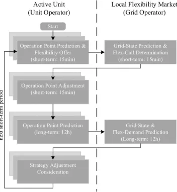
Since local flexibility markets are still in the development, the procedures, time-frames, market roles and flexibility products are not generally defined yet. In this paper a general procedure according to Fig.1 is proposed, considering it as a starting solution for the iterative optimization based on results of the simulation model.
Figure 1. Flexibility market procedure
Within the confined grid district of the local flexibility market, the active units at each node, which may be individual or aggregated, dispatchable loads and/or generators as well as energy storages, provide a short-term (minutes) and long-term (hours) operation point prediction. Passive units provide core data and measurement values for a prediction by the grid operator. Furthermore a unit can provide an offer for the possible flexibility during the next short-term period. Based on the predicted grid state and the short-term offer of the different flexibility suppliers, the grid operator runs the optimization and activates the necessary, cost-optimal amount of DGS.
According to the signal of the grid operator, the unit operators adjust their operation point and thereby avoid a critical grid state. Afterwards a long-term operation point prediction is exchanged with the grid operator. By receiving a long-term prediction on the DGS demand, the unit operators are enabled to adjust their operation strategy in order to participate in further auctions or use their flexibility for other purposes. The procedure starts over for the next period. The current approach uses a 15 min short-term period, due to the smallest tradeable unit on the energy markets and a 12 h long-term period as a trade-off between prediction accuracy and reaction time.
B. Requirements and Assumptions of the Proposal
The proposed design of the local flexibility procedure is related with several technical requirements. The considered grid district needs to be equipped with a Smart Grid system, allowing the real-time-observation and control of the grid. The Smart Grid system has to be extended by a market platform which handles all processes of the local flexibility market.
Furthermore, reliable load and infeed prediction systems need to be developed or adapted for distribution level. To allow further analysis, these requirements are primarily assumed to be fulfilled.
III. SIMULATION MODEL
The simulation of the local flexibility market behavior is based on a two domain model. The top level modelling principle is the strict distinction between the domains of the distribution grid operator and the unit operators to take account of the legal unbundling of the energy market and the grid.
During states of uncritical grid operation, all units behave according to their individual operation strategy. Only during predicted critical situations, the DSO provides incentives for the change of the unit’s operation point. The frameworks for the two modelling domains are illustrated in Fig. 2.
Figure 2. Model domains
The interface parameters of both model domains are the predicted fixed operation points of a unit divided into active Local Flexibility Market
(Grid Operator) Active Unit
(Unit Operator)
Operation Point Prediction &
Flexibility Offer (short-term: 15min)
Grid-State Prediction &
Flex-Call Determination (short-term: 15min)
Operation Point Adjustment (short-term: 15min)
Operation Point Prediction
(long-term: 12h) Grid-State &
Flex-Demand Prediction (Long-term: 12h)
Strategy Adjustment Consideration
Start
next short-term period
Unit Operator Model
Energy Demand & Supply Technical
Module Operation Strategy
Economic Module
Grid Operator Model
State Prediction Module FlexMarket Module State Control Module
Unit Domain Interface Grid Domain
𝑃𝑃𝑓𝑓𝑓𝑓𝑓𝑓𝑓𝑓𝑐𝑐𝑐𝑐𝑓𝑓 𝑓𝑓, 𝑄𝑄𝑓𝑓𝑓𝑓𝑓𝑓𝑓𝑓𝑐𝑐𝑐𝑐𝑓𝑓𝑓𝑓 𝑃𝑃𝑓𝑓𝑓𝑓𝑓𝑓𝑓𝑓𝑓𝑓, 𝑄𝑄𝑓𝑓𝑓𝑓𝑓𝑓𝑓𝑓𝑓𝑓 𝑃𝑃𝑓𝑓𝑓𝑓𝑓𝑓𝑓𝑓𝑚𝑚𝑓𝑓𝑚𝑚 ,𝑚𝑚𝑐𝑐𝑓𝑓, 𝑄𝑄𝑓𝑓𝑓𝑓𝑓𝑓𝑓𝑓𝑚𝑚𝑓𝑓𝑚𝑚 ,𝑚𝑚𝑐𝑐𝑓𝑓
𝐶𝐶𝑓𝑓𝑓𝑓𝑓𝑓𝑓𝑓𝑃𝑃 , 𝐶𝐶𝑓𝑓𝑓𝑓𝑓𝑓𝑓𝑓𝑄𝑄
power 𝑃𝑃𝑓𝑓𝑓𝑓𝑓𝑓𝑓𝑓𝑓𝑓and reactive power 𝑄𝑄𝑓𝑓𝑓𝑓𝑓𝑓𝑓𝑓𝑓𝑓, the minimum and maximum potential power flexibility 𝑃𝑃𝑓𝑓𝑓𝑓𝑓𝑓𝑓𝑓𝑚𝑚𝑓𝑓𝑚𝑚,𝑚𝑚𝑚𝑚𝑓𝑓 and 𝑄𝑄𝑓𝑓𝑓𝑓𝑓𝑓𝑓𝑓𝑚𝑚𝑓𝑓𝑚𝑚,𝑚𝑚𝑚𝑚𝑓𝑓 and the cost functions for providing the flexibility 𝐶𝐶𝑓𝑓𝑓𝑓𝑓𝑓𝑓𝑓𝑃𝑃,𝑄𝑄 for a time- interval ∆𝑡𝑡. Furthermore the results of the flexibility dispatch
𝑃𝑃𝑓𝑓𝑓𝑓𝑓𝑓𝑓𝑓𝑐𝑐𝑚𝑚𝑓𝑓𝑓𝑓 and 𝑄𝑄𝑓𝑓𝑓𝑓𝑓𝑓𝑓𝑓𝑐𝑐𝑚𝑚𝑓𝑓𝑓𝑓 are exchanged between the domains. The values
for the fixed and flexible active and reactive power can be both positive and negative depending on if a unit is providing or consuming power, the form of flexibility to change the operation point (generation or load, increase or decrease) and the power factor of a unit.
The unit operator domain can contain models of different complexity for active and passive units. Technology specific operation strategies, restrictions and parameters are handled within each unit model, exchanging only the predicted fixed and flexible power demand/supply with the grid operator model. Different examples of unit operator models are presented in section B.
A. Grid Operator Model
The grid operator model contains a complete grid structure model with the branch and node parameters of the specific grid section using the power system simulation environment of MATPOWER [15]. The software provides a powerful set of functions including AC and DC power flow and optimal power flow algorithms for symmetrical systems. OPF calculations are normally used to determine the operation point of various generation facilities at minimum total cost while covering a constant demand and considering the limits of the generators and the grid. Further applications are the minimization of losses and the increase of operating reserves on transmission level [16]. In this approach the OPF will be adapted to determine the operation points of several flexibility options, in order to avoid critical grid states on distribution level.
The grid operator aggregates the interface parameters of all units of the grid for each interval ∆𝑡𝑡 and preprocess them to be suitable for an Optimal-Power-Flow grid calculation. The fixed operation points 𝑃𝑃𝑓𝑓𝑓𝑓𝑓𝑓𝑓𝑓𝑓𝑓𝑓𝑓 and 𝑄𝑄𝑓𝑓𝑓𝑓𝑓𝑓𝑓𝑓𝑓𝑓𝑓𝑓 for the aggregated units at each node 𝑓𝑓 ∈ {2, . . , 𝑚𝑚𝑚𝑚} are considered as constant ‘demand’
(positive and negative sign) and the flexibility limits 𝑃𝑃𝑓𝑓𝑓𝑓𝑓𝑓𝑓𝑓𝑓𝑓,𝑚𝑚𝑓𝑓𝑚𝑚,𝑚𝑚𝑚𝑚𝑓𝑓
and 𝑄𝑄𝑓𝑓𝑓𝑓𝑓𝑓𝑓𝑓𝑓𝑓,𝑚𝑚𝑓𝑓𝑚𝑚,𝑚𝑚𝑚𝑚𝑓𝑓 of all flexibility options at the nodes 𝑓𝑓 ∈ {2, . . , 𝑚𝑚𝑚𝑚}
to be the operation limits of variable ‘generators’ (positive and negative sign). The operation set point of each flexibility is set to zero. The piecewise-linear cost functions 𝐶𝐶𝑓𝑓𝑓𝑓𝑓𝑓𝑓𝑓𝑃𝑃,𝑄𝑄 are equivalent to the cost functions of generation facilities in standard OPF applications with the extension of positive costs for negative power flexibility (e.g. RES curtailment). Furthermore the substation to superordinate grid level (𝑓𝑓 = 1) is used as the slack node and modelled as a generator with infinite positive and negative generation limits −∞ < 𝑃𝑃𝑓𝑓𝑓𝑓𝑓𝑓𝑓𝑓𝑓𝑓=1, 𝑄𝑄𝑓𝑓𝑓𝑓𝑓𝑓𝑓𝑓𝑓𝑓=1 < ∞ and zero costs
𝐶𝐶𝑓𝑓𝑓𝑓𝑓𝑓𝑓𝑓𝑓𝑓=1,𝑃𝑃,𝑄𝑄= 0. These assumptions lead to the adaption of the
standard OPF objective function of [15] to (1).
𝑉𝑉,Θ,Pminflex,𝑄𝑄𝑓𝑓𝑓𝑓𝑓𝑓𝑓𝑓� �𝐶𝐶𝑓𝑓𝑓𝑓𝑓𝑓𝑓𝑓𝑖𝑖,𝑃𝑃 �𝑃𝑃𝑓𝑓𝑓𝑓𝑓𝑓𝑓𝑓𝑖𝑖 � + 𝐶𝐶𝑓𝑓𝑓𝑓𝑓𝑓𝑓𝑓𝑖𝑖,𝑄𝑄�𝑄𝑄𝑓𝑓𝑓𝑓𝑓𝑓𝑓𝑓𝑖𝑖 ��
𝑛𝑛𝑚𝑚 𝑖𝑖=1
(1) The equality constrains are the power balance equations for the (𝑚𝑚𝑚𝑚× 1)-vectors of all nodes with 𝑉𝑉 being the voltage magnitude and Θ the voltage angle.
𝑷𝑷𝒏𝒏𝒏𝒏𝒏𝒏𝒏𝒏(𝑽𝑽, 𝚯𝚯) + 𝑷𝑷𝒇𝒇𝒇𝒇𝒇𝒇𝒏𝒏𝒏𝒏− 𝑷𝑷𝒇𝒇𝒇𝒇𝒏𝒏𝒇𝒇= 𝟎𝟎 (2)
𝑸𝑸𝒏𝒏𝒏𝒏𝒏𝒏𝒏𝒏(𝑽𝑽, 𝚯𝚯) + 𝑸𝑸𝒇𝒇𝒇𝒇𝒇𝒇𝒏𝒏𝒏𝒏− 𝑸𝑸𝒇𝒇𝒇𝒇𝒏𝒏𝒇𝒇= 𝟎𝟎 (3)
The inequality constraints consider the regular current flow limits of all branches 𝑰𝑰𝒎𝒎𝒎𝒎𝒇𝒇in (4),
|𝑰𝑰(𝑽𝑽, 𝚯𝚯)| − 𝑰𝑰𝒎𝒎𝒎𝒎𝒇𝒇≤ 𝟎𝟎 (4)
and the variable limits adapt to:
𝑉𝑉𝑖𝑖,𝑚𝑚𝑖𝑖𝑛𝑛≤ 𝑉𝑉𝑖𝑖≤ 𝑉𝑉𝑖𝑖,𝑚𝑚𝑚𝑚𝑓𝑓 (5)
𝑃𝑃𝑓𝑓𝑓𝑓𝑓𝑓𝑓𝑓𝑖𝑖,𝑚𝑚𝑖𝑖𝑛𝑛≤ 𝑃𝑃𝑓𝑓𝑓𝑓𝑓𝑓𝑓𝑓𝑖𝑖 ≤ 𝑃𝑃𝑓𝑓𝑓𝑓𝑓𝑓𝑓𝑓𝑖𝑖,𝑚𝑚𝑚𝑚𝑓𝑓 (6) 𝑄𝑄𝑓𝑓𝑓𝑓𝑓𝑓𝑓𝑓𝑖𝑖,𝑚𝑚𝑖𝑖𝑛𝑛≤ 𝑄𝑄𝑓𝑓𝑓𝑓𝑓𝑓𝑓𝑓𝑖𝑖 ≤ 𝑄𝑄𝑓𝑓𝑓𝑓𝑓𝑓𝑓𝑓𝑖𝑖,𝑚𝑚𝑚𝑚𝑓𝑓 . (7) After the parametrization of the state prediction module for the current interval, an OPF-calculation will be executed. As long as all branch currents (4) and node voltages (5) remain within their limits, the result of the cost minimization (1) will be the adaption of the (slack) generator at the substation node in order to balance the power flow equations (2) and (3). The operation point of the flexibility options will remain zero, as their dispatch is always more expensive than the costless power exchange with the superordinate grid. The grid is operating under non-critical conditions. If the predicted operation points of all nodes do lead to any limit value violations, the slack generator cannot solve them, since the slack node voltage is constant. In this case, the result of the OPF is the cost-optimal dispatch of the given flexibility options in the grid district. The results are sent to all unit models in order to initiate the change of the operation point.
If the offer on the local flexibility market was not sufficient to avoid the problem, the OPF will not converge. In this case or if the DGS is not performed by the unit operator, the real-time state control will intervene directly (red traffic light phase).
B. Unit Operator Model
Within the unit domain, the models may differ depending on the technology, process or aggregation they represent. The modular structure of the simulation framework allows easy additions or adaptions of unit models. In order to provide the necessary background for the following case study, three examples of unit operator models are presented briefly. For simplification, the further description of the unit operator models is limited to active power flexibility.
1) CHP plant with gas storage
The first unit operator model represents a combined heat and power plant (CHP) with an additional gas storage, as it can be found for sewage gas on wastewater treatment plants or other biogas plants. The primary energy supply is the variable production of biogas in the fermenter expressed as the volumetric gas flow rate 𝑄𝑄𝐺𝐺(𝑡𝑡). The internal energy demand of the plant will be not further discussed and expressed by the total power demand 𝑃𝑃𝑓𝑓𝑓𝑓𝑚𝑚(𝑡𝑡). The operation mode of the generator is mainly driven by the state-of-charge (SOC) of the gas storage.
Technical constrains of the model are the minimum and maximum SOC of the gas storage 𝑆𝑆𝑆𝑆𝐶𝐶𝐺𝐺𝐺𝐺𝑚𝑚𝑓𝑓𝑚𝑚,𝑚𝑚𝑚𝑚𝑓𝑓, the generator operation limits 𝑃𝑃𝑔𝑔𝑓𝑓𝑚𝑚𝑚𝑚𝑓𝑓𝑚𝑚,𝑚𝑚𝑚𝑚𝑓𝑓 and the gas to power conversion efficiency 𝜂𝜂𝐶𝐶𝐶𝐶𝑃𝑃 of the plant. The dynamic behavior of the SOC can be expressed by (8).
𝑆𝑆𝑆𝑆𝐶𝐶𝐺𝐺𝐺𝐺(t + Δ𝑡𝑡) = 𝑆𝑆𝑆𝑆𝐶𝐶𝐺𝐺𝐺𝐺(𝑡𝑡) + 𝑄𝑄𝐺𝐺(𝑡𝑡)Δ𝑡𝑡 − 1
𝜂𝜂𝐶𝐶𝐶𝐶𝑃𝑃𝑃𝑃𝑔𝑔𝑓𝑓𝑛𝑛(t)Δ𝑡𝑡 s.t. (a) 𝑆𝑆𝑆𝑆𝐶𝐶𝐺𝐺𝐺𝐺𝑚𝑚𝑖𝑖𝑛𝑛≤ 𝑆𝑆𝑆𝑆𝐶𝐶𝐺𝐺𝐺𝐺≤ 𝑆𝑆𝑆𝑆𝐶𝐶𝐺𝐺𝐺𝐺𝑚𝑚𝑚𝑚𝑓𝑓
(b) 𝑃𝑃𝑔𝑔𝑓𝑓𝑛𝑛𝑚𝑚𝑖𝑖𝑛𝑛≤ 𝑃𝑃𝑔𝑔𝑓𝑓𝑛𝑛≤ 𝑃𝑃𝑔𝑔𝑓𝑓𝑛𝑛𝑚𝑚𝑚𝑚𝑓𝑓
(8)
The generator operation mode is chosen based on the predicted development of 𝑆𝑆𝑆𝑆𝐶𝐶𝐺𝐺𝐺𝐺(t + Δ𝑡𝑡) under the primary assumption that the generator operation would remain as it was, considering two switching thresholds (𝑆𝑆𝑇𝑇1 and 𝑆𝑆𝑇𝑇2).
𝑃𝑃𝑔𝑔𝑓𝑓𝑛𝑛(𝑡𝑡) = �
𝑃𝑃𝑔𝑔𝑓𝑓𝑚𝑚𝑚𝑚𝑐𝑐𝑓𝑓 ∀ 𝑆𝑆𝑆𝑆𝐶𝐶𝐺𝐺𝐺𝐺(t + Δ𝑡𝑡) > 𝑆𝑆𝑇𝑇2
𝑃𝑃𝑔𝑔𝑓𝑓𝑚𝑚𝑚𝑚𝑛𝑛𝑚𝑚 ∀ 𝑆𝑆𝑇𝑇1< 𝑆𝑆𝑆𝑆𝐶𝐶𝐺𝐺𝐺𝐺(t + Δ𝑡𝑡) < 𝑆𝑆𝑇𝑇2
0 ∀ 𝑆𝑆𝑆𝑆𝐶𝐶𝐺𝐺𝐺𝐺(t + Δ𝑡𝑡) < 𝑆𝑆𝑇𝑇1
(9)
After the operation point is predefined, the interface parameters are calculated according (10)-(12), with the definition of a negative 𝑃𝑃𝑓𝑓𝑓𝑓𝑓𝑓𝑓𝑓𝑓𝑓 to be infeed to the grid and negative sign of 𝑃𝑃𝑓𝑓𝑓𝑓𝑓𝑓𝑓𝑓 to be infeed reduction respectively load increase.
𝑃𝑃𝑓𝑓𝑖𝑖𝑓𝑓𝑓𝑓𝑓𝑓(𝑡𝑡) = 𝑃𝑃𝑓𝑓𝑓𝑓𝑚𝑚(𝑡𝑡) − 𝑃𝑃𝑔𝑔𝑓𝑓𝑛𝑛(𝑡𝑡) (10)
𝑃𝑃𝑓𝑓𝑓𝑓𝑓𝑓𝑓𝑓𝑚𝑚𝑖𝑖𝑛𝑛(𝑡𝑡) = −𝑃𝑃𝑔𝑔𝑓𝑓𝑛𝑛(𝑡𝑡) (11)
𝑃𝑃𝑓𝑓𝑓𝑓𝑓𝑓𝑓𝑓𝑚𝑚𝑚𝑚𝑓𝑓(𝑡𝑡) =𝑃𝑃𝑔𝑔𝑓𝑓𝑚𝑚𝑚𝑚𝑐𝑐𝑓𝑓− 𝑃𝑃𝑔𝑔𝑓𝑓𝑛𝑛(𝑡𝑡) (12) In order to complete the set of interface parameters, the cost functions for the minimal and maximal flexibility offer need to be calculated. In this model linear cost functions are employed according Fig. 3.
Figure 3. Cost functions
Individual conditions, cost calculations and market strategies of each unit operator may result in complex economic modelling modules, which are beyond the scope of the paper.
In this unit operator model, the flexibility is assumed to be offered for a constant service price 𝑓𝑓𝑝𝑝𝑝𝑝.
𝐶𝐶𝑓𝑓𝑓𝑓𝑓𝑓𝑓𝑓𝑝𝑝 = 𝑓𝑓𝑝𝑝𝑝𝑝�𝑃𝑃𝑓𝑓𝑓𝑓𝑓𝑓𝑓𝑓� (13)
2) Wind and photovoltaic power plant
Wind and photovoltaic power plants are lacking an inherent energy storage, therefore the electricity generation is driven by the weather conditions. Nevertheless they can offer flexibility through their operation concept. Negative flexibility can be provided through curtailment and even positive flexibility through a power increase from throttled operation.
Both technologies are modelled with the same unit operator model. The provided wind and solar power 𝑃𝑃𝑤𝑤𝑓𝑓𝑚𝑚𝑓𝑓/𝑃𝑃𝑃𝑃 is converted into electrical power with regard to the conversion efficiency of the plant 𝜂𝜂𝑝𝑝𝑓𝑓𝑚𝑚𝑚𝑚𝑝𝑝and the state-dependent or independent throttle operation factor 𝑓𝑓𝑝𝑝ℎ.
𝑃𝑃𝑔𝑔𝑓𝑓𝑛𝑛(𝑡𝑡) = 𝜂𝜂𝑝𝑝𝑓𝑓𝑚𝑚𝑛𝑛𝑝𝑝𝑓𝑓𝑝𝑝ℎ𝑃𝑃𝑤𝑤𝑖𝑖𝑛𝑛𝑓𝑓 𝑝𝑝𝑝𝑝⁄ (t) (14) s.t. 𝑃𝑃𝑔𝑔𝑓𝑓𝑛𝑛𝑚𝑚𝑖𝑖𝑛𝑛≤ 𝑃𝑃𝑔𝑔𝑓𝑓𝑛𝑛≤ 𝑃𝑃𝑔𝑔𝑓𝑓𝑛𝑛𝑚𝑚𝑚𝑚𝑓𝑓
The flexibility parameters are determined analogously to the CHP-model by (10)-(12).
Assuming that the units sold their predicted energy production already, the curtailed amount needs to be balanced through a purchase on the intraday spot market. Therefore the prices for curtailment are derived from the intraday prices 𝑓𝑓𝑝𝑝𝑝𝑝𝑓𝑓𝑚𝑚𝑝𝑝𝑝𝑝𝑚𝑚
of the energy exchange plus an individual operator margin 𝑓𝑓𝑚𝑚𝑚𝑚𝑝𝑝𝑔𝑔. 𝐶𝐶𝑓𝑓𝑓𝑓𝑓𝑓𝑓𝑓𝑝𝑝 = 𝑓𝑓𝑝𝑝𝑝𝑝𝑖𝑖𝑛𝑛𝑝𝑝𝑝𝑝𝑚𝑚𝑓𝑓𝑚𝑚𝑚𝑚𝑝𝑝𝑔𝑔�𝑃𝑃𝑓𝑓𝑓𝑓𝑓𝑓𝑓𝑓� (15) 3) Power-to-Gas plant
Power-to-Gas plants (PtG) separate water into oxygen and hydrogen via electrolysis. From the power system perspective, PtG plants with hydrogen infeed to the gas grid can be considered as simple flexible loads. Therefore the electrical power demand in this unit operator model only depends on the operation strategy. In this example, technical constrains are neglected and the individual operation strategy is assumed to be driven by the participation in the balancing power market.
The plant operator offers the nominal power demand of the PtG unit 𝑃𝑃𝑓𝑓𝑓𝑓𝑚𝑚𝑚𝑚𝑛𝑛𝑚𝑚 in weekly auctions as negative secondary control power in the high tariff (HT) and low tariff (LT) time windows with the marginal operation costs 𝐶𝐶𝑚𝑚𝑚𝑚𝑝𝑝𝑔𝑔. If the bid is accepted in week 𝑘𝑘 ∈ {1. .52}, the unit is committed 𝑓𝑓𝑘𝑘,𝐶𝐶𝐻𝐻,𝐿𝐿𝐻𝐻𝑐𝑐𝑛𝑛𝑚𝑚 = 1 during the tariff time window for a whole week and may not participate in other markets. During time windows with no commitment
𝑓𝑓𝑘𝑘,𝐶𝐶𝐻𝐻,𝐿𝐿𝐻𝐻𝑐𝑐𝑛𝑛𝑚𝑚 = 0, the unit can provide the total nominal power 𝑃𝑃𝑓𝑓𝑓𝑓𝑚𝑚𝑛𝑛𝑛𝑛𝑚𝑚
as DGS. Thus, the calculation of 𝑃𝑃𝑓𝑓𝑓𝑓𝑓𝑓𝑓𝑓𝑚𝑚𝑓𝑓𝑚𝑚 changes from (11) to (16).
𝑃𝑃𝑓𝑓𝑓𝑓𝑓𝑓𝑓𝑓𝑓𝑓 and 𝑃𝑃𝑓𝑓𝑓𝑓𝑓𝑓𝑓𝑓𝑚𝑚𝑚𝑚𝑓𝑓 emerge from (10) and (12) with 𝑃𝑃𝑔𝑔𝑓𝑓𝑚𝑚= 0.
𝑃𝑃𝑓𝑓𝑓𝑓𝑓𝑓𝑓𝑓𝑚𝑚𝑖𝑖𝑛𝑛(𝑘𝑘) = �−𝑃𝑃𝑓𝑓𝑓𝑓𝑚𝑚𝑚𝑚𝑛𝑛𝑚𝑚 ∀ 𝑓𝑓𝑘𝑘,𝐻𝐻𝑇𝑇,𝐿𝐿𝑇𝑇𝑐𝑐𝑛𝑛𝑚𝑚 = 0
0 ∀ 𝑓𝑓𝑘𝑘,𝐻𝐻𝑇𝑇,𝐿𝐿𝑇𝑇𝑐𝑐𝑛𝑛𝑚𝑚 = 1 (16)
The price assumptions in this operator model are equivalent to the wind and photovoltaic power operator model in (15).
IV. CASE STUDY
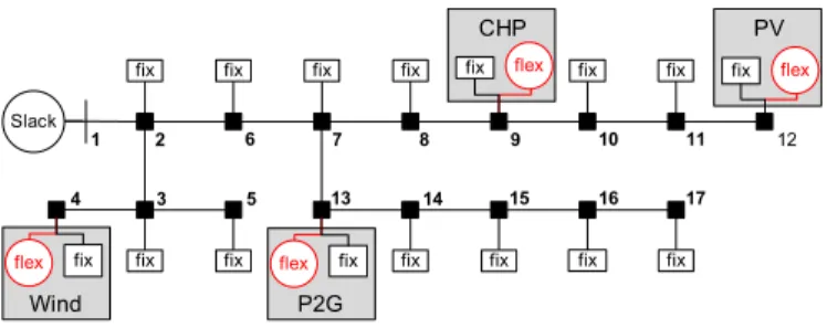
The application of the simulation model will be presented in a case study for a 17-node 10kV medium voltage rural grid district in Germany. A future scenario (2035+) for the penetration of DG and the development of loads is applied to the existing grid. The structure of the grid is shown in Fig. 4.
Figure 4. 17-node 10kV medium voltage grid
The overall cable length adds up to 13km supplying a total load of 2 MVA and an installed generation capacity of 2 MW wind, 800 kWp of distributed PV(including a 300 kWp single
𝑃𝑃𝑓𝑓𝑓𝑓𝑓𝑓𝑓𝑓𝑚𝑚𝑓𝑓𝑚𝑚 𝑃𝑃𝑓𝑓𝑓𝑓𝑓𝑓𝑓𝑓𝑚𝑚𝑐𝑐𝑓𝑓 𝑃𝑃𝑓𝑓𝑓𝑓𝑓𝑓𝑓𝑓[𝑘𝑘𝑘𝑘]
𝐶𝐶𝑓𝑓𝑓𝑓𝑓𝑓𝑓𝑓𝑃𝑃 [€]
fix fix fix fix fix fix fix
fix fix fix
fix
flex
2
4 3 5
6 7 8 9 10 11 12
13 14 15 16 17
CHP
1
fix flex PV
flex fix Wind
flex fix P2G
fix fix
Slack
unit at node 12) and 160 kW CHP. The parameters of the four flexibility suppliers are summarized in TABLE I.
TABLE I. PARAMETERS FLEXIBILITY OPTIONS
Node Operator
Model Installed
Capacity Price Margin
factor
4 Wind 2000 kW Intraday + margin 1.2
9 CHP 160 kW 5 €/MW (constant) -
12 PV 300 kWp Intraday + margin 1.1
13 P2G 200 kW Intraday + margin 1.05
The other nodes are not participating on the local flexibility market but still influence the power-flow and flexibility demand through their fixed load/infeed. The slack voltage at the HV/MV substation (node 1) is maintained constantly with 𝑉𝑉𝑓𝑓=1= 1.03 𝑉𝑉𝑚𝑚𝑛𝑛𝑚𝑚. The tolerable voltage limits for all other nodes are set to 𝑉𝑉𝑓𝑓.𝑚𝑚𝑓𝑓𝑚𝑚= 0.97 𝑉𝑉𝑚𝑚𝑛𝑛𝑚𝑚 and 𝑉𝑉𝑓𝑓.𝑚𝑚𝑚𝑚𝑓𝑓= 1.05 𝑉𝑉𝑚𝑚𝑛𝑛𝑚𝑚.
The simulation will be executed with a time-resolution of
∆𝑡𝑡 = 15 𝑚𝑚𝑓𝑓𝑚𝑚 for the duration of one year. The infeed and load time series are based on measured values of the specific grid district for a whole year, scaled with the installed capacities of the scenario. The time-series of the sewage gas production is also based on measured values and the gas storage capacity as well as the conversion efficiency correspond to the existing units in the district. Reactive power of each unit is calculated by constant power factors and not assumed to be flexible. The applied market prices are the publicly available results of the balancing market and the European Energy Exchange for 2014.
A. Detailed Results of 12-hour time span
In this specific grid and supply task constellation, only violations of the upper voltage boundary occur. Thus, considering only active power adjustments, an increase of load or an infeed reduction (i.e. negative flexibility) can solve the problem.
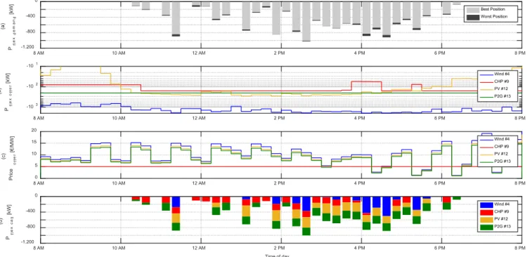
Primarily, the simulation results for 12 hours of a day with critical grid conditions are presented. Fig. 5 (a) shows the active power flexibility demand for each 15-min interval between 8 AM and 8 PM, which is determined by test calculations at each node. In this example, the lowest demand at the “best”
node position and the highest demand at the “worst” node position only vary slightly. Therefore, all flexibility suppliers are theoretically able to contribute grid services.
The amount of active power flexibility each unit can offer is displayed in Fig. 5 (b). It depends on the energy supply (wind and solar power) and the operation strategy and varies in each interval. The flexibility is offered for the prices shown in Fig. 5 (c). The price courses of the units ‘Wind #4’, ‘PV #12’ and
‘P2G #13’ are the same, since they are all connected to the intraday prices. Only the amplitude differs depending on the margin factor. The prices of ‘CHP #9’ remain constant.
Finally, Fig. 5 (d) shows the cost-optimal coverage of the flexibility demand through the different flexibility options as the result of the OPF-calculation. The problematic grid conditions only occur during times with high amounts of wind power infeed. Therefore, the curtailment of the wind power plant is the only flexibility option, which could solve all problems individually. But from the cost perspective, it is not the optimal solution in this example. Since the influence of the node position is minor, the order of calls can be derived from the price offer. During most intervals, ‘CHP #9’ offers the cheapest DGS and the curtailment ‘Wind #4’ is the most expensive option. It can be easily seen, that the flexibility of
‘Wind #4’ is only called, when the offer of all other options is not sufficient anymore. The only exception are several time intervals between 4 PM and 8 PM, where the prices of the intraday trading drops below the constant price offer of the CHP. In these cases, the CHP flexibility is not called.
Figure 5. Flexibility (a) demand, (b) offer, (c) price, (d) call - (12-hour simulation)
8 AM 10 AM 12 AM 2 PM 4 PM 6 PM 8 PM
(a) Pflexdemand [kW]
-1.200 -800 -400
0
Best Position Worst Position
8 AM 10 AM 12 AM 2 PM 4 PM 6 PM 8 PM
(b) Pflexoffer [kW]
-103 -102 -101
Wind #4 CHP #9 PV #12 P2G #13
8 AM 10 AM 12 AM 2 PM 4 PM 6 PM 8 PM
(c) Priceoffer [€/MW]
0 5 10 15 20
Wind #4 CHP #9 PV #12 P2G #13
Time of day
8 AM 10 AM 12 AM 2 PM 4 PM 6 PM 8 PM
(d) Pflexcall [kW]
-1.200 -800 -400 0
Wind #4 CHP #9 PV #12 P2G #13
B. Results of one year simulation
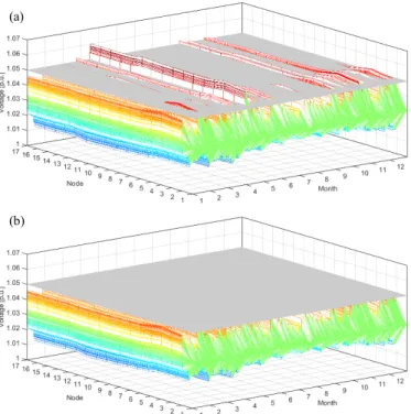
The simulation of a whole year in 15 min steps showed, that in this specific case, violations of the upper voltage boundary at any node of the grid occurred only during 73.75 h (0.84 % of the year). In all cases, the offered flexibility options were sufficient to solve the problems. All node voltages over the whole year are shown in Fig. 6 (a) without DGS calls and therefore with violations of the upper voltage boundary (grey layer) and in Fig. 6 (b) with DGS.
Figure 6. Node voltages (a) without DGS (b) with DGS (one year simulation) The annual results for the described case (Case A) are summarized in TABLE II. The number of individual calls are listed as well as the amount of energy that is curtailed or shifted and the costs for each supplier. All options are called in the course of the year.
As mentioned above, the wind power plant in this example is capable of solving all limit value violations individually by curtailment. In order to compare this option, a second case (Case B) is calculated, assuming ‘Wind #4’ to be the only flexibility option. The price assumptions correspond to Case A.
TABLE II. ANNUAL RESULTS (CASE A&B) Flex
Option Case A (all options) Case B (wind only) Calls
[h] Energy [MWh] Cost
[€] Calls
[h] Energy [MWh] Cost Wind 30.5 2.6 78 73.75 10.4 421 [€]
CHP 55.5 4.1 82 - - -
PV 15.25 1.4 51 - - -
P2G 26.5 3.5 128 - - -
Total 73.75 11.6 339 73.75 10.4 421 The comparison of both cases shows the economic advantage of the local flexibility market (Case A) over the straight forward curtailment of RES (Case B). Furthermore it needs to be considered, that the amount of energy that is drawn by the CHP and P2G plant is used for gas production
respectively stored as sewage gas. The amount of energy that is curtailed by the RES is lost for conversion in to electrical power.
However, the results are highly sensitive to the price assumptions and a well-performing local flexibility market needs price competition between the suppliers of flexibility.
Additionally the implementation and operation costs need to be considered and compared to other options of grid operation and enhancement, in order to make further economical statements.
Nevertheless, the presented OPF approach provides a helpful tool, to simulate the behavior of different flexibility options on a local market.
V. APPLICATION OUTLOOK
The results of the analysis show that using local flexibility markets may help to apply DGS and therefore to reduce the cost-intensive grid enhancement at distribution level. The below-mentioned aspects may be the subject of further research.
A. Further research on the performance of local flexibility markets
The implementation of local flexibility markets at lower voltage levels could mean a usage of active power that is both network stabilizing and market economy driven. Unlocking such flexibility markets by installing measurement and automation technology may be associated with increased costs initially. It is therefore likely that operators of local flexibility markets will enter further short-term markets to maximize their revenues. The interaction with other short-term markets in this case represents one of the central challenges that should be considered at an early stage as part of the design of local flexibility markets.
It can be assumed that the individual operator has no preference for or against a market. He will offer his commodity where it can achieve the highest price with a similar effort. The various markets – the power balancing market, the power exchange market, and the flexibility market – compete for the same commodity (positive or negative power adjustment). The individual markets trade with varying lead times. A trade on the energy balancing market the day before is no longer available on the flexibility market on the next day. By contrast, trading on the intraday spot market will take place simultaneously or slightly before the trading on the flexibility market. While only providers of large capacities are permitted on the power exchange and the energy balancing markets, the flexibility market primarily targets small and medium capacities. Further research should reveal the extent to which conflicting interests of the different markets may become economically problematic [7].
A potential conflict could arise, for example, when a transmission system operator requests a power increase to stabilize grid frequency in a given grid section, thereby causing local off-limit voltages. Then the distribution system operators would react by decreasing power infeed in the relevant grid section, which in turn would reduce the grid frequency. In order to avoid such conflicts of interest, the sequence in which capacities may be accessed must be clearly defined. Here the (a)
(b)
idea of a traffic light for grid capacity can help to structure the interaction between the markets.
B. Implementation in an autonomous Smart Grid system Activity on the local flexibility market needs to be automated as far as possible in order to process the large amount of information available. In the grid domain (see Fig. 2), this would require the implementation of a decentralized automation system. Such monitoring and control systems, however, are still rare in distribution grids in Germany.
Current decentralized automation systems for distribution grids are limited in most cases to indicate green and red traffic light states with regard to grid capacity (congestion management) [3]. The yellow state in which the local flexibility market operates, requires forecasting supply and demand with a high temporal and spatial resolution. The development of a function which uses historical grid states and weather forecasts to predict the flexibility market should be the subject of further work. Future automation systems should also have an adequate degree of self-sufficiency and adaptability, so that the control center is not overloaded by the implementation of a local flexibility market.
VI. CONCLUSION
This paper suggests to establish local flexibility markets as a possible option to coordinate distribution grid services in order to avoid critical grid operation states. To allow further analysis on the design, procedures, benefits and disadvantages of local flexibility markets, a basic approach is presented to simulate the operational behavior of these markets and their participants.
A two domain modelling framework for the simulation of local flexibility markets considers the strict distinction between the individual operation strategies of each unit and the interests of the distribution grid operator. In situations of predicted critical grid conditions, the operators interact in order to find a minimal cost solution to avoid the problems. The modular construction of the modelling framework allows an easy extension with further flexibility options in addition to the presented models for PV and wind power plants, CHP plants with gas storage and P2G plants. Furthermore the existing models are quickly adaptable to different operation strategies and technical constrains.
The cost-minimal commitment of the different flexibility options is calculated by an Optimal-Power-Flow algorithm, considering flexibility suppliers as variable generators. The presented case study of a rural 10kV medium voltage grid shows the functionality of this approach and confirms the assumption that critical grid states only occur a few times a year. Therefore solving these problems using distribution grid services is appropriate. In most cases using a combination of different flexibility options is more cost-effective than the curtailment of a single distributed generator only.
Overall, the approach proved to be helpful for further analysis of local flexibility markets. Additional improvements and developments, like the development of more complex operation strategies and economic modules, and the comparison
to other operational or constructional grid enhancement options, will be subject to further work.
REFERENCES
[1] L. E. Jones, “Renewable Energy Integration – Practical Management of Variability, Uncertainty and Flexibility in Power Grids” Academic press, 2015.
[2] Dena – German Energy Agency, “dena Distribution Grid Study / dena Verteilnetzstudie” [Online]. Available: http://www.dena.de/fileadmin/
user_upload/Projekte/Energiesysteme/Dokumente/denaVNS_Abschluss bericht.pdf
[3] C. Oerter and N. Neusel-Lange, "LV-grid automation system — A technology review," PES General Meeting | Conference & Exposition, 2014 IEEE, National Harbor, MD, 2014, pp. 1-5.
[4] European Distribution System Operators for Smart Grid (EDSO),
„Flexibility: The role of DSOs in tomorrow’s electricity market,“ EDSO Position Paper [Online]. Available: http://www.edsoforsmartgrids.eu/
wp-content/uploads/public/EDSO-views-on-Flexibility-FINAL-May- 5th-2014.pdf
[5] C. Zhang et al., "A flex-market design for flexibility services through DERs," Innovative Smart Grid Technologies Europe (ISGT EUROPE), 2013 4th IEEE/PES, Lyngby, 2013, pp. 1-5.
[6] R. Apel, V. Berg, B. Fey, K. Geschermann, W. Glaunsinger, A. v.
Scheven, M. Stötzer and S. Wanzek, “Regionale Flexibilitätsmärkte”, VDE ETG, Frankfurt am Main, Germany, Sep. 2014.
[7] J. Meese, J. Winkler, N. Neusel-Lange, M. Zdrallek, J. Antoni, M.
Stiegler, W. Friedrich, „Markets for flexibility supporting the intelligent grid in the yellow traffic light phase“, in Proc. 2015 ETG-Fachtagung:
Von Smart Grids zu Smart Markets, P 6.3.
[8] K. Heussen, S. Koch, A. Ulbig and G. Andersson, "Unified System- Level Modeling of Intermittent Renewable Energy Sources and Energy Storage for Power System Operation," in IEEE Systems Journal, vol. 6, no. 1, pp. 140-151, March 2012.
[9] A. Ulbig and G. Andersson, "Analyzing operational flexibility of electric power systems," Power Systems Computation Conference (PSCC), 2014, Wroclaw, 2014, pp. 1-8.
[10] A. Hoke, A. Brissette, S. Chandler, A. Pratt and D. Maksimović, "Look- ahead economic dispatch of microgrids with energy storage, using linear programming," Technologies for Sustainability (SusTech), 2013 1st IEEE Conference on, Portland, OR, 2013, pp. 154-161.
[11] E. Sortomme and M. A. El-Sharkawi, "Optimal Power Flow for a System of Microgrids with Controllable Loads and Battery Storage," Power Systems Conference and Exposition, 2009. PSCE '09. IEEE/PES, Seattle, WA, 2009, pp. 1-5.
[12] B. HomChaudhuri, M. Kumar and V. Devabhaktuni, "Market based approach for solving optimal power flow problem in smart grid,"
American Control Conference (ACC), 2012, Montreal, QC, 2012, pp.
3095-3100.
[13] BDEW – German Association of Energy and Water Industries, „BDEW Roadmap – Realistic Steps for the Implementation of Smart Grids in Germany,“ [Online]. Available: https://www.bdew.de/internet.nsf/id/
816417E68269AECEC1257A1E0045E51C/$file/Endversion_BDEW- Roadmap_englisch.pdf
[14] BDEW – German Association of Energy and Water Industries, „Smart Grid Traffic Light Concept – Design of the amber phase,“ Discussion paper [Online]. Available: https://www.bdew.de/internet.nsf/id/
816417E68269AECEC1257A1E0045E51C/$file/Smart%20Grid%20Tr affic%20Light%20Concept.pdf
[15] R. D. Zimmerman, C. E. Murillo-Sanchez and R. J. Thomas,
"MATPOWER: Steady-State Operations, Planning, and Analysis Tools for Power Systems Research and Education," in IEEE Transactions on Power Systems, vol. 26, no. 1, pp. 12-19, Feb. 2011.
[16] N. Rau, "Introduction," in Optimization Principles: Practical Applications to the Operation and Markets of the Electric Power Industry , 1, Wiley-IEEE Press, 2003, pp.1-5.