The Measurement- and Model-based Structural Analysis for Damage Detection

(1)

Veröffentlichungen der DGK

Ausschuss Geodäsie der Bayerischen Akademie der Wissenschaften

Reihe C Dissertationen Heft Nr. 844

Cheng-Chieh Wu

The Measurement- and Model-based Structural Analysis for Damage Detection

München 2020

Verlag der Bayerischen Akademie der Wissenschaften

ISSN 0065-5325 ISBN 978-3-7696-5256-7

Diese Arbeit ist gleichzeitig veröffentlicht in:

Universitätsbibliothek der Technischen Universität Berlin http://dx.doi.org/10.14279/depositonce-8845, Berlin 2019

(2)

(3)

Veröffentlichungen der DGK

Ausschuss Geodäsie der Bayerischen Akademie der Wissenschaften

Reihe C Dissertationen Heft Nr. 844

The Measurement- and Model-based Structural Analysis for Damage Detection

Von der Fakultät – Planen Bauen Umwelt der Technischen Universität Berlin zur Erlangung des akademischen Grades Doktor der Ingenieurwissenschaften (Dr.-Ing.)

genehmigte Dissertation

Vorgelegt von

Dipl.-Ing. Cheng-Chieh Wu

Geboren am 08.10.1983 in Taipeh

München 2020

Verlag der Bayerischen Akademie der Wissenschaften

ISSN 0065-5325 ISBN 978-3-7696-5256-7

Diese Arbeit ist gleichzeitig veröffentlicht in:

Universitätsbibliothek der Technischen Universität Berlin http://dx.doi.org/10.14279/depositonce-8845, Berlin 2019

(4)

Adresse der DGK:

Ausschuss Geodäsie der Bayerischen Akademie der Wissenschaften (DGK) Alfons-Goppel-Straße 11 ● D – 80539 München

Telefon +49 – 331 – 288 1685 ● Telefax +49 – 331 – 288 1759 E-Mail post@dgk.badw.de ● http://www.dgk.badw.de

Promotionsausschuss:

Vorsitzender: Prof. Dr. phil. nat. Jürgen Oberst Gutachter: Prof. Dr.-Ing. Frank Neitzel

Prof. Dr.-Ing. Andreas Eichhorn

Univ.-Prof. Dipl.-Ing. Dr.techn. Werner Lienhart Prof. Dr.-Ing. Werner Daum

Tag der wissenschaftlichen Aussprache: 20.03.2019

die Veröffentlichung oder Teile daraus auf photomechanischem Wege (Photokopie, Mikrokopie) zu vervielfältigen

ISSN 0065-5325 ISBN 978-3-7696-5256-7

(5)

Summary

The present work is intended to make a contribution to the monitoring of civil engineering structures. The detection of damage to structures is based on the evaluation of spatially and temporally distributed hybrid measurements.

The acquired data can be evaluated purely geometrically or physically. It is preferable to do the latter, since the cause of damage can be determined by means of geometrical-physical laws in order to be able to intervene in time and ensure the further use of the structures. For this reason, the continuum mechanical field equations in conjunction with the finite element method and hybrid measurements are combined into a single evaluation method by the adjustment calculation. This results in two challenges.

The first task deals with the relationship between the finite element method and the method of least squares. The finite element method solves certain problem classes, which are described by a system of elliptical partial differential equations. Whereas the method of least squares solves another class of problems, which is formulated as an overdetermined system of equations. The striking similarity between both methods is known since many decades. How- ever, it remains unresolved why this resemblance exists. The contribution is to clarify this by examining the variational calculus, especially with regard to its methodological procedure. Although the well-knownGauss-Markov model within the method of least squares and the finite element method solve inherently different problem classes, it is shown that both methods can be derived by following the same methodological steps of the variational calculus. From a methodical viewpoint, this implies that both methods are not only similar, but actually the same. In addition, it is pointed out where a possible cross-connection to other methods exists.

The second task introduces a Measurement- and Model-based Structural Analysis (MeMoS) by integrating the finite element method into the adjustment calculation. It is shown in numerical examinations how this integrated analysis can be used for parameter identification of simple as well as arbitrarily shaped structural components. Based on this, it is examined with which observation types, with which precision and at which location of the structure these measurements must be carried out in order to determine the material parameters as precisely as possible. This serves to determine an optimal and economic measurement set-up. With this integrated analysis, a substitute model of a geometrically complex structure can also be determined. The issue of the detection and localisation of damage within a structure is studied by means of this structural analysis. The Measurement and Model-based Structural Analysis is validated using two different test setups, an aluminum model bridge and a bending beam.

(6)

(7)

Zusammenfassung

Die vorliegende Arbeit soll einen Beitrag zur Überwachung von Ingenieurbauwerken leisten. Die Detektion von Schäden an Bauwerken basiert auf der Auswertung von räumlich und zeitlich verteilten Hybridmessungen. Die erfassten Daten können rein geometrisch oder physikalisch ausgewertet werden. Letzteres ist vorzuziehen, da die Schadensursache mittels geometrisch-physikalischer Gesetze ermittelt werden kann, um rechtzeitig eingreifen und die weitere Nutzung der Bauwerke sicherstellen zu können. Aus diesem Grund werden die kontinuumsmechani- schen Feldgleichungen in Verbindung mit der Finite-Elemente-Methode und Hybridmessungen durch die Ausglei- chungsrechnung zu einer einzigen Auswertemethode kombiniert. Dabei ergeben sich zwei Aufgabenstellungen.

Die erste Aufgabe beschäftigt sich mit der Beziehung zwischen der Finite-Elemente-Methode und der Ausglei- chungsrechnung. Die Finite-Elemente-Methode löst bestimmte Problemklassen, die durch ein System elliptischer partieller Differentialgleichungen beschrieben werden. Während die Methode der kleinsten Quadrate eine weitere Klasse von Problemen löst, die als ein überdeterminiertes Gleichungssystem formuliert ist. Die auffallende Ähnlich- keit zwischen den beiden Methoden ist seit vielen Jahrzehnten bekannt. Es bleibt jedoch ungeklärt, warum diese Ähnlichkeit besteht. Der Beitrag soll dies klären, indem die Variationsrechnung im Hinblick auf ihr methodisches Vorgehen untersucht wird. Obwohl das bekannteGauss-Markov-Modell innerhalb der Methode der kleinsten Quadrate und die Finite-Elemente-Methode inhärent unterschiedliche Problemklassen lösen, wird gezeigt, dass beide Methoden durch die gleichen methodischen Schritte der Variationsrechnung abgeleitet werden können. Aus methodischer Sicht bedeutet dies, dass beide Methoden nicht nur ähnlich, sondern sogar gleich sind. Außerdem wird darauf hingewiesen, wo eine mögliche Querverbindung zu anderen Methoden besteht.

Die zweite Aufgabenstellung stellt eine Messungs- und Modellbasierte Strukturanalyse (MeMoS) durch die Integra- tion der Finite-Elemente-Methode in die Ausgleichungsrechnung vor. In numerischen Untersuchungen wird gezeigt, wie diese integrierte Analyse zur Parameteridentifikation sowohl einfacher als auch beliebig geformter Struk- turbauteile eingesetzt werden kann. Darauf aufbauend wird untersucht, mit welchen Beobachtungstypen, mit welcher Genauigkeit und an welcher Stelle der Struktur diese Messungen durchgeführt werden müssen, um die Ma- terialparameter möglichst genau zu bestimmen. Dies dient der Ermittlung eines optimalen und wirtschaftlichen Messaufbaus. Mit dieser integrierten Analyse kann auch ein Ersatzmodell einer geometrisch komplexen Struktur ermittelt werden. Die Frage der Erkennung und Lokalisierung von Schäden innerhalb einer Struktur wird mit Hilfe dieser Strukturanalyse behandelt. Die Messungs- und Modellbasierte Strukturanalyse wird mit zwei verschiedenen Testaufbauten, einer Aluminium-Modellbrücke und einem Biegebalken, validiert.

(8)

(9)

Preface

The research presented in this dissertation was supported by the PhD funding programme “Menschen, Ideen, Strukturen” (“People, Ideas, Structures”) of theBundesanstalt für Materialforschung und -prüfung(BAM). In addition, theTechnische Universität Berlin(TUB) has enriched this doctoral programme through its infrastruc- ture. I am grateful to the members of the appraisal committee Professor Dr. W. Daum, Professor Dr. F. Neitzel and Dr. K. Brandes for giving me the opportunity to write this dissertation.

I want to thank Professor Dr. W. Daum for his supervision and generous support. As the director of his department and deputy director of several departments, he nevertheless took time for me every week to discuss the progress of my dissertation. He was understanding and open to my concerns and gave me valuable advice and suggestions.

Furthermore, I want to thank Professor Dr. F. Neitzel for his kind support and guidance throughout this time. In Professor Dr. F. Neitzel I had a liberal supervisor who gave me the freedom to conduct my research according to my own ideas, while giving me encouragement and counsel. I appreciate his openness to accept even a non-geodesist like me to join his institute. Especially, he created an environment that promotes cooperation between different disciplines, in my case geodesy and continuum mechanics, in which this dissertation could develop. I appreciate his sense of humour, which has reduced my nervousness and anxiety. Nevertheless, he has always critically and rigorously questioned my chains of reasoning and derivations and provided valuable feedback.

I am grateful to Dr. K. Brandes for his visits and the insight into his wisdom and knowledge about bridges.

Furthermore, I would like to express my gratitude to Professor Dr. A. Eichhorn, Professor Dr. W. Lienhart and Pro- fessor Dr. W. Daum for the kind acceptance of the appraisal of this dissertation and also to Professor Dr. J. Oberst for accepting the chairmanship of the dissertation procedure.

I would like to thank my numerous colleagues at BAM and TUB: I want to express my appreciation to H. Kohlhoff, M. Fischer, J. Erdmann and S. Schendler who supported me in the planning and construction of the model bridge.

In the group of Terrestrial Laser Scanning I would like to thank Dr. D. Wujanz and J. Feng. I wish to thank D. Kadoke and M. Burger in the Photogrammetry group. I am also grateful that my colleagues have kept my body in a healthy state, Dr. M. Bartholmai, U. and T. Braun, S. Fritzsche, G. Von-Drygalski and D. Hüllmann. I am especially indebted to the latter for additionally keeping my mind in a sane state. Many thanks to Dr. F. Richter for proofreading. Great thanks to A. Barthelmeß for helping me to order the books from various libraries all over Germany. Special thanks to B. Eule who took care of bureaucratic matters for me. My gratitude goes to my office colleague K.-P. Gründer who took care of me. My sincere thanks go to G. Malissiovas for the endless discussion about adjustment calculation. And I thank P. Neumann as a former office colleague.

My cordial thanks go to my colleagues who made it possible for me to obtain follow-up financing, Dr. E. Köppe, Dr. R. Helmerich, Dr. M. Bartholmai and Professor Dr. W. Daum.

I am particularly indebted to my mentor and office colleague at TUB S. Weisbrich. He took care of me when I was in a tough situation, both at work and privately. That’s how he kept me sane, so I could finish my dissertation. It is also valuable to me that we often have fierce and passionate disputes about mathematics in engineering sciences.

Finally, I would like to thank my parents, A.-T. Wu (吳安德) and M.-H. Wu Liu (吳劉美華), for their support and encouragement as hard-working chefs in their own Taiwanese restaurantBeef House(牛稼莊) in Berlin throughout my education. I would also like to dedicate this dissertation to my grandmothers, C.-H. Liu Wu (劉吳秋紅) and Y.-C. Yang (楊玉珍), and my late grandfathers, K.-L. Wu (吳桂林, a former chef) and P.-K. Liu (劉炳國, a former policeman). In particular, my late grandfather, P.-K. Liu, wanted me to do my doctorate.

Berlin, August 2019 Cheng-Chieh Wu (吳正覺)

(10)

(11)

Genealogy

ChristianFelixKlein 25. Apr. 1849 in Düsseldorf 22. Jun. 1925 in Göttingen

Carl LouisFerdinandvon Lindemann 12. Apr. 1852 in Hannover 6. Mar. 1939 in München

DavidHilbert 23. Jan. 1862 in Königsberg

14. Feb. 1943 in Göttingen

BernhardBaule 4. May 1891 in Münden

5. Apr. 1976 in Graz

HelmutMoritz 1. Nov. 1933 in Graz

DieterLelgemann 31. Aug. 1939 in Essen-Steele

18. Aug. 2017 in Berlin

SvetozarPetrovic 25. Jan. 1952 in Zagreb

FrankNeitzel 3. Sep. 1968 in Münster

Cheng-ChiehWu 8. Oct. 1983 in Taipeh JuliusPlücker

16. Jun. 1801 in Elberfeld 22. May 1868 in Bonn Christian LudwigGerling

10. Jul. 1788 in Hamburg 15. Jan. 1864 in Marburg JohannCarl FriedrichGauß

30. Apr. 1777 in Braunschweig 23. Feb. 1855 in Göttingen

RudolfOtto Sigismund Lipschitz 14. May 1832 in Königsberg

7. Oct. 1903 in Göttingen JohannPeter Gustav LejeuneDirichlet

13. Feb. 1805 in Düren 5. May 1859 in Göttingen Siméon DenisPoisson

21. Jun. 1781 in Pithiviers 25. Apr. 1840 in Paris

Jean BaptisteJosephFourier 21. Mar. 1768 in Auxerre

16. May 1830 in Paris Joseph-Louisde Lagrange

25. Jan. 1736 in Turin 10. Apr. 1813 in Paris

LeonhardEuler 15. Apr. 1707 in Basel 18. Sep. 1783 in Paris

Source: Mathematics Genealogy Project

(12)

(13)

List of Figures

1.1 A flowchart for classifyingMeasurement- and Model-based Structural Analysisas a dynamic deformation model or as an integrated deformation analysis according toChrzanowskiet al. (1990);

the structure to be examined in the sense of system theory (top part);Measurement- and Model-

based Structural Analysis(bottom part) 4

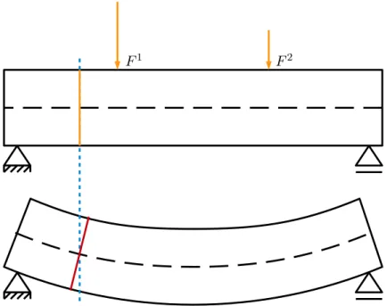
2.1 A four-point bending test apparatus. 33

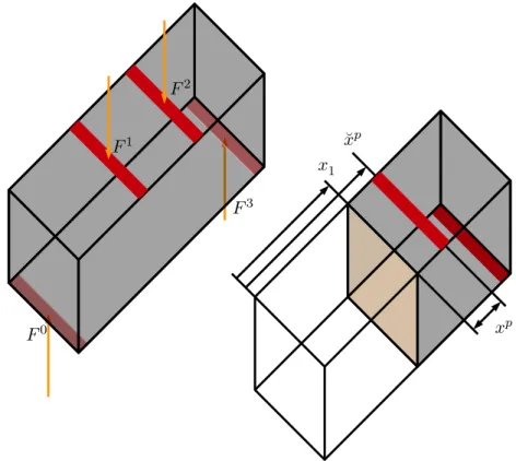
2.2 The Method of Sections generates afree-body diagramfor revealing the inner stresses within a beam. The forcesF^p are applied on the rectangular traction areas with depthdand widthw

which are marked in red. 34

2.3 Explanation of the semi-inverse method. 35

2.4 Explanation of the semi-inverse method. 36

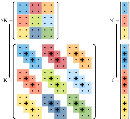
2.5 (Left) Assembly of the total stiffness matrixKfrom the element matrices^ζK. (Right) Assembly of the total load vectorffrom the element load vectors^ζ+1f. 52 4.1 The representation of the trial functionΦ=P

i

c_iX_ias a neuron network. 84

5.1 Basic principle of the approaches for material parameter determination of complex samples as pro-

posed byEichhorn(2005) andLienhart(2007) 86

5.2 The bending momentM 87

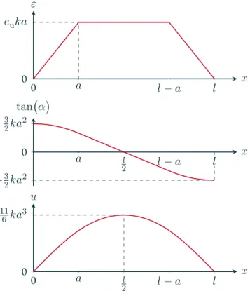
5.3 The exact solution of the beam differential equation, from top to bottom: strainε, tangent of the inclinationtan α

, displacementu 89

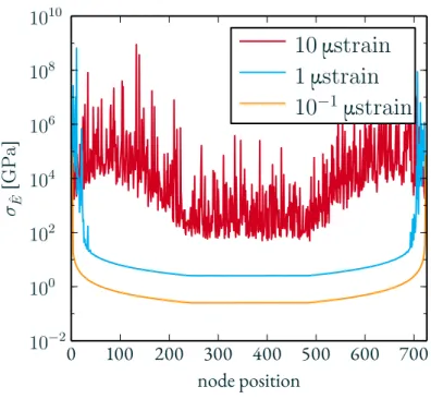
5.4 Precision of the estimated elastic modulusσ_ˆ

E depending on sensor position and three different

precisions of a displacement sensor 92

precisions of a tilt sensor 92

precisions of a strain sensor 93

E depending on number of sensors with fixed precision 93 5.8 Beam defects due to geometric changes or material changes (left) are simulated by material degra-

dation (right) 94

5.9 Examination of predefined damage scenarios 96

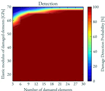
5.10 Damage detection depending on material degradation (change of elastic modulus) and number

of damaged elements 96

5.11 Damage localisation depending on material degradation (change of elastic modulus) and number

of damaged elements 97

5.12 A six-point bending test apparatus for an aluminium beam specimen. This test device was partly

enhanced by scrap such as lead battery, dumbbell, plastic box. 98

5.13 Deflection lines of the undamaged beam subjected to various external forces and the measured displacement from photogrammetry (top left), the corresponding residuals (top right), the complete residuals in one representation (middle) and the corresponding standardised residuals (bottom) 101

LIST OF FIGURES iii

(16)

5.14 The position where damage is induced. 104 5.15 Undamaged beam subjected to external weight of5.491 kg, adjusted deflection line and measured

displacementu₄(top left), the corresponding residuals as line representation (top right), the corresponding residuals as bar representation (middle), and the standardised residuals of the displace-

ment observations (bottom); no damage detected 105

5.16 Undamaged beam subjected to external weight of17.825 kg, adjusted deflection line and measured displacementu₃(top left), the corresponding residuals as line representation (top right), the corresponding residuals as bar representation (middle), and the standardised residuals of the displacement observations (bottom); damage detected, false alarm 106 5.17 Damaged beam subjected to external weight of3.546 kg, adjusted deflection line and measured

displacementu₂₁(top left), the corresponding residuals as line representation (top right), the corresponding residuals as bar representation (middle), and the standardised residuals of the displace-

ment observations (bottom); no damage detected 107

5.18 Damaged beam subjected to external weight of7.114 kg, adjusted deflection line and measured displacementu₂₅(top left), the corresponding residuals as line representation (top right), the corresponding residuals as bar representation (middle), and the standardised residuals of the displace-

ment observations (bottom); damage detected 108

5.19 Damaged beam subjected to external weight of7.114 kg, displacement measurementsu₂₅; elastic moduli of the beam (top), the residuals of the observed unknowns (middle), the standardised residuals of the observed unknowns (bottom); damage localisation at element nodeζ = 15 109 5.20 Damaged beam subjected to external weight of3.561 kg, adjusted deflection line and measured

displacementu₂₇(top left), the corresponding residuals as line representation (top right), the corresponding residuals as bar representation (middle), and the standardised residuals of the displace-

5.21 Damaged beam subjected to external weight of3.561 kg, displacement measurementsu₂₇; elastic moduli of the beam (top), the residuals of the observed unknowns (middle), the standardised residuals of the observed unknowns (bottom); damage localisation at element nodeζ = 22 111 5.22 Damaged beam subjected to external weight of17.808 kg, adjusted deflection line and measured

displacementu₃₁(top left), the corresponding residuals as line representation (top right), the corresponding residuals as bar representation (middle), and the standardised residuals of the displace-

5.23 Damaged beam subjected to external weight of17.808 kg, displacement measurementsu₃₁; elastic moduli of the beam (top), the residuals of the observed unknowns (middle), the standardised residuals of the observed unknowns (bottom); damage localisation at element nodeζ = 22 113 5.24 Aluminium profile with a geometrical complex inner structure can be substituted by an approxi-

mate model 116

5.25 (a) Undeformed substitute model; (b) Undeformed original model; (c) Deformed original model;

(d) Overlay comparison between the undeformed (grey) and deformed (red transparent) body of the original model; (e) Displacement field; (f) Overlay comparison between the undeformed (grey)

and deformed (red transparent) body of the substitute model 117

5.26 An “inverted” compression test inx₁-axis direction on the surface normal inx₁-axis direction;top leftA normal stressσ₁₁is applied to the original sample;top rightA normal stressσ₁₁is applied to the substitute sample;bottom leftAn overlay comparison between the original and substitute samples in a deformed state;bottom rightParameter 1 and also due to symmetry considerations

parameter 1 can be determined in this test 120

5.27 An “inverted” compression test inx₂-axis direction on the surface normal inx₂-axis direction;top leftA normal stressσ₂₂is applied to the original sample;top rightA normal stressσ₂₂is applied to the substitute sample;bottom leftAn overlay comparison between the original and substitute samples in a deformed state;bottom rightParameter 1 and also due to symmetry considerations

parameter 1 can be determined in this test 121

iv LIST OF FIGURES

(17)

5.28 An “inverted” compression test inx₃-axis direction on the surface normal inx₃-axis direction;top leftA normal stressσ₃₃is applied to the original sample;top rightA normal stressσ₃₃is applied to the substitute sample;bottom leftAn overlay comparison between the original and substitute samples in a deformed state;bottom rightParameter 2 can be determined in this test 122 5.29 A simple shear test inx₂-axis direction on the surface normal inx₃-axis direction;top leftA shear

stressσ₂₃is applied to the original sample;top rightA shear stressσ₂₃is applied to the substitute sample;bottom leftAn overlay comparison between the original and substitute samples in a deformed state;bottom rightParameter 3 and also due to symmetry considerations parameter 3

can be determined in this test 123

5.30 A simple shear test inx₁-axis direction on the surface normal inx₃-axis direction;top leftA shear stressσ₁₃is applied to the original sample;top rightA shear stressσ₁₃is applied to the substitute sample;bottom leftAn overlay comparison between the original and substitute samples in a deformed state;bottom rightParameter 3 and also due to symmetry considerations parameter 3

can be determined in this test 124

5.31 A simple shear test inx₁-axis direction on the surface normal inx₂-axis direction;top leftA shear stressσ₁₂ is applied to the original sample;top rightA shear stressσ₁₂ is applied to the substitute sample;bottom leftAn overlay comparison between the original and substitute samples in a deformed state;bottom rightParameter 4 can be determined in this test 125 5.32 An uniaxial tensile test inx₁-axis direction on the surface normal inx₁-axis direction;top leftA

normal stressσ₁₁is applied to the original sample;top rightA normal stressσ₁₁is applied to the substitute sample;bottom leftAn overlay comparison between the original and substitute samples in a deformed state;bottom rightParameters 1 , 2 , 5 and 6 can be determined in this test 126 5.33 For the verification of the adjusted elastic parameters, a comparison between a original aluminium

beam with a substitute beam is being made 127

5.34 Overlay comparison between original aluminium (grey) beam and substitute beam (red, transparent); length of the beams:1520 mm; Three test set-ups:topThree-point bending test,middleone sided cantilever test andbottomdouble sided cantilever test; Three different forces:50 N(blue),

500 N(yellow) and5000 N(red) 127

5.35 Overlay comparison between original aluminium (grey) beam and substitute beam (red, transparent); length of the beams:700 mm; Three test set-ups:topThree-point bending test,middleone sided cantilever test andbottomdouble sided cantilever test; Three different forces:50 N(blue),

500 N(yellow) and5000 N(red) 128

5.36 The bridge specimen on the pedestal, approximately2147.6 Nwas applied 131 5.37 Terrestrial laser scanning of the bridge model, the coloured spheres indicate where screws are loos-

ened to cause damage, damage level 1: red spheres, damage level 2: red and yellow spheres, damage

level 3: red, yellow and blue spheres 133

5.38 Screws are released to induce artificial damages to the bridge model 134 5.39 The stiffness tensor has to be rotated in accordance to the different spatial orientations of the profiles 135 5.40 The standardised residuals of the observed unknownsNV_ζ for 598 chunks of the bridge speci-

men’s finite element model by evaluation of the displacement measurementsL₂, two different

perspectives of the bridge specimen (top and bottom) 142

5.41 The standardised residuals of the observed unknownsNV_ζ by evaluation of the displacement measurementsL₂ including the observed displacement vectors magnified 500 times, a profile is highlighted in green that indicates an additional displacement field induced by residual stress 143 5.42 The standardised residuals of the observed unknownsNV_ζ by evaluation of the displacement

measurementsL₃including the observed displacement vectors magnified 500 times 145 5.43 The standardised residuals of the observed unknownsNV_ζ by evaluation of the displacement

measurementsL₄including the observed displacement vectors magnified 500 times 146

LIST OF FIGURES v

(18)

(19)

List of Tables

4.1 An overview of the discussed methods. Gauss-Markovmodel (GMM), continuousGauss- Markovmodel (cGMM), finite element method (FEM), least squares finite element method

(LSFEM) 83

5.1 Specification of the four-point bending set-up and beam specimen for the finite element modelling. 90

5.2 Synthetic measurements on beam specimen 95

5.3 For each states, weights (m₁,m₂,m₃) were attached to the undamaged beam specimen andn_photo

images were taken. 99

5.4 For each states, weights (m₁,m₂,m₃) were attached to the damaged beam specimen andn_photo

images were taken. 102

5.5 The measurement data designation indicates whether the beam is actually damaged or undamaged, the displacement measurements setu_ifrom states⁰tos, the theoretical reference standard devi- ationσ₀, the empirical reference standard deviations₀, the test statisticχ²_r, the threshold value for all casesχ²_r,1−α = 44.985for redundancyr = 31and error probabilityα= 5 %, if it holds p :χ²_r > χ²_r,1−αthen rejectH₀ in favour ofH_A, the allegedly damaged finite elementζrespec- tively^ζEˆ, the ratior_el = ²²_ˆ^E^ˆ

E between the damaged and undamaged finite element,²²EˆandE,ˆ

the total attached weightsm 103

5.6 Results of original and substitute beams that are subjected to three-point bending tests (TP), dou- ble sided cantilever tests (DC) and single sided cantilever tests (SC) and the total computational

time (TCT) 129

5.7 Different spatial orientations of the aluminium profile 136

5.8 Calibration process of the reference state 139

5.9 Global test for different displacement measurements setsL_i, the theoretical reference standard deviationσ₀, the empirical reference standard deviations₀, the total redundancyr, test statistic χ²_r, threshold valueχ²_r,1−α, if it holdsχ²_r > χ²_r,1−αthen rejectH₀ in favour ofH_A 141

LIST OF TABLES vii

(20)

(21)

1 Prologue

Nothing shocks me. I’m a scientist.

– Dr. Henry Walton “Indiana” Jones, Jr., Indiana Jones and the Temple of Doom (1984)

Technical Diagnostics(Czichos2013) is concerned with diagnostic procedures and methods for the determination offaultsorfailuresin technical objects. The examination may revealsymptomsor evensyndromes(groups of symptoms) that indicate of abnormal condition. On a continuous or scheduled basis, the diagnosis can be carried out. The technical diagnostics may be principally broken down into two applications:Condition Monitoring(ISO 13372:20122012) andStructural Health Monitoring(SHM) (FarrarandWorden2013). Both diagnostics are dedicated to the acquisition of data and to the process of information that indicate the state of a technical object.

The scope of condition monitoring is mainly on machines, while the focus of structural health monitoring is set on civil engineering structures such as buildings, bridges, dams, main road, railways, processing plants, etc.

The objective of structural health monitoring is to guarantee the functionality, quality, reliability and safety of civil engineering structures. The important outcome from structural monitoring is to avoid catastrophic failures and unintended downtime, to identify suspicious behaviour before it becomes a problem, to support maintenance and overhaul management and to provide assistance to research and development for innovative structural designs and to standardised guidelines and practices. The monitoring procedure begins with data acquisition of structural behaviour to evaluate structural performance under designated environmental and operational conditions. Unex- pected results may indicate the damage or deterioration of the structure and can be a valuable indicator of the state or condition of the structure.

Daum(2013, p. 413 ff) specifies ageneric design procedurecommon to all structural health monitoring systems designs. This generic design process ultimately defines the basic concept ofmonitoringwhich can be summarised as:

1. characterisation of the structure and identification of the required measurands as well as of the significant parameters for damage evaluation,

2. selection of suitable sensors and data acquisition system, 3. application of an appropriate diagnostic method.

In this thesis, theMeasurement- and Model-based Structural Analysisfor early damage detection and localisation is presented following the term monitoring as defined above.

Firstly, the structural behaviour is described by means of a physical model. This in turn leads to field equations that connect theprimitive variablesto thematerial parametersas well as to a set ofboundary conditions. Mass density, velocity, temperature, electric field, magnetic flux density and their spatial and temporal derivatives are considered as primitive variables. The boundary conditions describe the environmental and operational effects on engineering structure. The material parameters characterise the substances which the structure is made of. The required measurands for structural health monitoring are identified by determining the quantities that can be measured in the field equations and in the boundary conditions. Material parameters are regarded as unmeasurable as they can only be drawn from observations of measurable quantities. Furthermore, they serve as a key feature for the damage evaluation.

Secondly, once the measurands have been identified, decisions regarding the selection of suitable sensors and data acquisition system have to be made based on the following three criteria: performance and quantity of sensors,

PROLOGUE 1

(22)

environmental sensor operating conditions and economical aspects. A model-basedsensitivity analysisis carried out to evaluate the impact of stochastic characteristics of sensors on the material parameters computation. The results of this analysis provide the information about the minimum requirement for the performance and quantity of sensors. Consequently, these results are used to assess the economic feasibility of a structural monitoring plan.

Thirdly and lastly, as stated inWordenet al. (2007), sensors are incapable to measure damage. However, from the measurements they collect, tangible features such as material parameters can be extracted. Then, structural damages are identified by comparing features from different states of the structure. In this comparison, hypothesis testings from statistical analysis are applied to detect and localise damages. The success rate of damage detection and localisation depends on the sensor precision, on the correctness of the physical modelling and on the structural damage severity. In aMonte Carlo simulationthis dependence can be clarified beforehand.

Therefore, theMeasurement- and Model-based Structural Analysiscan be placed as part of the group of technical diagnostics. However, from a civil engineering perspective, the four main aims in structural health monitoring are

1. the detection, 2. the localisation, 3. the causes and

4. the prognoses of damages

in a structure. This perspective does not necessary contradict the generic design procedure of the technical diagnostics, rather thephysicalcharacterisation / description of the structure becomes utmost important. While structural damages can be detected and localised by non-physical approaches, the causes of damages and the following prognoses rely heavily on a physical model. Even though, theMeasurement- and Model-based Structural Analysisdoes not claim to be the ultimate method that can determine all the causal links between measurements and the sources of damages, the presented analysis lays down the fundamental framework that will allow progressing toward the goal in further researches. Hence, theMeasurement- and Model-based Structural Analysisrequires a coherent evaluation between physical model and measurements by means of an adjustment method with the capability to assess statistically the results in regard of precision and reliability.

Related Works

According toWelschandHeunecke(2001), engineering surveys are involved in all phases of the life cycle phase of a structure: Planning phase, construction, commissioning, operation and maintenance, renovation or demo- lition. Deformation measurementsbetween commissioning, operation and maintenance are of particular importance. The main task of the deformation measurements and its corresponding analysis in these phases are to obtain a detailed and relevant description of the structure in order to examine its condition. The aim and purpose of the monitoring measures is the early detection of damages, failures and hazards for operational safety in order to be able to take measures in good time. Monitoring measures are only one aspect that improves operational safety.

Therefore engineering surveying is unable to cover all aspects, however it is an important component. As a result, the monitoring of structures today is a multidisciplinary task.

In accordance withWelschandHeunecke(2001), there are fourdeformation models: congruence, kinematic, static and dynamic model. Each individual model is discussed as follows.

Conventional deformation analysisaims to clarify the geometry of the structure and its motion geometry by captur- ing the structural body with discrete points at a given point in time. The causes of the movement are not examined.

The captured motion of each point is then used to reconstruct the displacement and deformation of the structure.

Thecongruence modelsin conventional deformation analysis is a classical approach for monitoring a structure. The geometry of the structure is compared at two or more points in time. A statistical test is then carried out to determine whether a deformation has occurred or not. For example,Heuneckeet al. (2013, p. 488 ff) examine a control point network that spans the surface of the structure. By means of stochastic evaluations, significant position changes of the points of the network are determined from different states of the structure.

2 PROLOGUE

(23)

In the conventional deformation analysis the congruence models can be understood as a special case of the so-called kinematic models. In these models, the motion functions of the discrete points are explicitly estimated from quasi- continuous measurements. The determined time-dependent motion functions can then be further analysed. For example,Welsch(1986) shows the determination of the velocity and strain rate field from continuous position measurements of a geodetic network. The results were developed with regard to the assessment of structure move- ments or distortions.

While conventional methods examine the spatial and temporal deformation changes of a structure purely geometrically, theadvanced deformation analysisalso considers the cause of deformation. Both the physical properties and the external influences of the structure are taken into account as the reason for the deformation. In terms of system theory, the causal forces are input parameters which are transformed by the structure as a transfer function into the resulting deformation as output quantities. This creates a causal chain that is referred to as adynamic system. The modelling of this dynamic system is a complex issue that can only be successfully addressed through interdisciplinary collaboration. The advanced deformation analysis is formally divided into static and dynamic models, whereby the static variants can be understood as a special case of the dynamic cases.

First, thestatic modelsevaluate between different structural states in which the structure is in equilibrium with forces. The forces acting on the structure can differ between the equilibrium states. The advantage over the congruence model is that this makes it possible to compare deformation states of the structure under different external conditions in order to detect possible damage to the structure. For example,Brandeset al. (2012) evaluate two static states of a wooden bridge, one loaded with external forces and one unloaded. With the help of discrete displacement measurements on a wooden bridge and a mechanical model, combined with an evaluation method of the adjustment calculation withLagrangemultipliers, drilling damage could be detected.

Second, Thedynamic modelsevaluate a structure in the non-equilibrium state. The structural motion under time- dependent influences is examined. For example, the vibration behaviour of the structure can be examined in order to determine possible damage. TheAmbient Vibration MonitoringfromWenzelandPichler(2005) analyses distinct dynamic structural behaviour. When a structure, such as a bridge, is monitored, it can be observed that the structure is constantly in motion due to the excitation by the environment. And for a brief moment, the structure might be relieved of the environmental influences. At that moment, a decaying vibration is observed. This behaviour suggests that a structure can be adequately described by a (physical) spring-damping system, i. e., structural deformation can be decomposed into two parts: reversible and irreversible. Deformation that recovers completely after removal of the external influences is considered as reversible and as such this part can be represented as spring components within a structural system. A remaining deformation is referred to as irreversible part that is imagined in a system as damping components. TheForced Vibration Analysisalso analyses the dynamic structural behaviour as described above, see for exampleBrinckerandVentura(2015). The difference is that controlled vibration is induced.

If both the cause and the reactions of a structure are measurable, the transfer function can be determined from them. The formulation of a suitable mathematical representation of the transfer function of a dynamic system (dynamic and static models) is calledsystem identification. The identification of the transfer function may be based on physical reasoning. This is calledparametric identificationin the terms of system theory. Alternatively, the system can be identified without rational justification by an empirical mathematical description which is referred to asnon-parametric identification. In both cases, however, suitable input and output data must be available for a successful system identification.

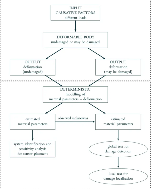
A flowchart in Fig. 1.1, based on the idealized flowchart in Chrzanowski et al. (1990), is used to classify Measurement- and Model-based Structural Analysiswith regard to deformation analysis. In Fig. 1.1, the upper part represents the structure to be examined. A deformable body, such as a structure, is deformed by external loads.

Without loss of generality, two observers are shown who measure the deformation of the structure in different states. The first observer measures the deformation of the structure under defined loads in an essentially arbitrary reference state at initial times for which a damage-free state can be assumed. The second observer measures the deformation of the same structure at a later time under possible changed loads and under possible changed conditions of the structure. The lower part representsMeasurement- and Model-based Structural Analysis. By means of continuum mechanics, a deterministic relationship is established between the two quantities, material parameters and structural deformation, in the form of a system of partial differential equations. Using the finite element method, the partial differential equations are converted into a system of equations, so that it is then possible to integrate

PROLOGUE 3

(24)

INPUT

CAUSATIVE FACTORS different loads

DEFORMABLE BODY undamaged or may be damaged

OUTPUT deformation (undamaged)

DETERMINISTIC modelling of

material parameters – deformation

OUTPUT deformation (may be damaged)

estimated material parameters

system identification and sensitivity analysis for sensor placment

estimated material parameters

global test for damage detection

local test for damage localisation observed unknowns

Figure 1.1: A flowchart for classifyingMeasurement- and Model-based Structural Analysis as a dynamic deformation model or as an integrated deformation analysis according toChrzanowskiet al. (1990); the structure to be examined in the sense of system theory (top part);Measurement- and Model-based Structural Analysis (bottom part)

4 PROLOGUE

(25)

them into the adjustment calculation. This makes it possible to estimate the material parameters from the deformation measurements (system identification). In addition, it is possible to perform sensitivity analyses using synthetic deformation measurements to identify the optimal sensor placement. The estimated material parameters from the undamaged state of the structure can be used asobserved unknownstogether with deformation measurements from later epochs to detect and localize possible damage to the structure.

In the sense ofWelschandHeunecke(2001) andChrzanowskiet al. (1990) it can be stated thatMeasure- ment- and Model-based Structural Analysiscan be regarded as a dynamic deformation model or as an integrated deformation analysis. Due to computer limitations, there is a trade-off between dealing with dynamic topics or geometric complexity. Although the theoretical foundations for the treatment of time-dependent problems are discussed, this work deals only with the static issue. This decision has no influence on the fact thatMeasurement- and Model-based Structural Analysisis still a dynamic model.

TheMeasurement- and Model-based Structural Analysisis to be applied to bridge monitoring. In terms of Struc- tural Health Monitoring, this dissertation implements a complete process of strategies and techniques for damage detection and localisation of engineering structures as proof-of-concept:

• construction of a small test bridge,

• acquisition of the bridge behaviour with suitable sensors,

• determination of damage-relevant quantities from the measurements,

• statistical analysis of the extracted parameters for the determination of the current structural condition.

Scope of the Work

Structural Health Monitoringrequires interdisciplinary knowledge from various parts of engineering. The scope of this dissertation is to identify damage with a rigorous analysis by fusing the fundamentals belonging to continuum mechanics and geodesy. On one hand, continuum mechanics provides the framework to describe the behaviour of the structure in terms of the relationship between the primitive field quantities to the boundary conditions and to the material parameters. On the other hand, adjustment theory in geodesy provides methods to determine unknown parameters from observations and fixed values as well as to evaluate the results in regard to precision and reliability. The presentedMeasurement- and Model-based Structural Analysisis based on the expertise of these two engineering fields. Material parameters characterise and quantify physical properties of matters. Changes that occur to the substances are noticed in alteration in these parameters. In this thesis, material constants are used as main features for the assessment of early damage detection on structures. The challenge is to extract and to assess material parameters from the measurements of different epochs. The stochastic evaluation of material parameters leads to the detection of damage. If defects is detected in the structure, individual local material parameters are further analysed to locate the damage. In summary, the objectives ofMeasurement- and Model-based Structural Analysiscan be addressed in the context of structural health monitoring as follows: Damage is to be detected and localised as well as explained by a decrease in the material parameter value. Since the focus here is on early detection of damage, the damage prognosis is omitted in this dissertation.

Aforesaid, structural health monitoring combines know-how from different fields of engineering. It should be generally understood that to include everything about engineering science would go beyond the scope in this dissertation. Even if there is a limitation to materials, say steel, concrete, wood, that are the usual building materials, it is still impossible to complete this dissertation in a reasonable time. As a matter of fact, there are different types of material, and they behave differently under the same conditions. Therefore, there are individual departments, each is dealing with specialised material such as department for metallic materials, department for construction chemistry, department for biological materials, etc. The common feature of all building materials is that they behave in a linearly elastic manner. This idealisation is a necessary simplification that has to be made. Anything that significantly deviates from this assumption can be interpreted as damage. Certainly, damping elements that are installed on bridges to shift the resonance frequency would disturb this premise immensely. However, in further research as well as the ambient vibration monitoring already suggests, one can use linear viscoelasticity, combination of linear elasticity and linear viscosity, to characterise the building materials to overcome this limitation. In this

PROLOGUE 5

(26)

dissertation, the foundation for a general method for structural health monitoring is laid: Continuum mechanics is known for its generality to analyse physical systems in an axiomatic deductive way. While adjustment theory, in a broader sense, is a general method to convert mathematical and physical relationships into useful results. Both have the generalisation in common. The commitment in this work is to keep approaches to any given task as general as possible.

The finite element method and the least squares adjustment are essential for theMeasurement- and Model-based Structural Analysis. A more academic perspective in this dissertation deals with the relationship between those two methods. As stated inLienhart(2007), he referred in his dissertation that many geodesists already knew about the striking similarity between the mentioned methods. Analogies between finite element method and least squares adjustment were presented, but the mentioned geodesists failed to show that both methods can be derived from the so-calledvariational calculuseven though each method is apparently trying to solve different types of problems.

While the development of the finite element method is often considered coming from mechanics, it is shown here that finite element method should be seen as a part of the adjustment theory.

Scientific and Technological Significance

Approximation, optimisation, filtering, projection, biological evolution, genetic algorithm, machine learning, data encryption and decryption, data compression, building information modelling, industry 4.0, internet of things and many more are in no doubt inherently different. But, what if all these notions can be consolidated, to be precise, the methodological approaches that are attached to those notions, in a single unified method, a unified adjustment theory? The advantages lie ahead: One would be able to comprehend all these different ideas and concepts in an instant, because they are perceived as similar. The benefit would be that they could be combined and be applied for different engineering tasks. This could lead to new and innovative approaches. In a long run, it is a lucrative objective to show the connections between, at first sight, different methods. In a short-term, in this dissertation, the connections between the finite element method and least squares adjustment are tied by means of the calculus of variations. Both methods share inherently different notions, while the finite element method solves certain classes of problems described by a system of elliptic partial differential equations, the method of least squares solves another class of problems formulated as overdetermined system of equations. At the end of the day, both methods follow the very same methodological steps that were developed byLagrangeandEulerback in 1755. Theadjustment theoryis more than a main tool used only in geodesy. In this dissertation, adjustment theory is being extended by assimilation of variation calculus in the hope of unifying all known methods. The aim is to reach the ultimate method that can solve any mathematically describable problem. In the end, when liberated from the burden of the many confusing origins and being unified, it will be simply called:The Method.

The aims that are demanded by structural health monitoring can only be reached by interdisciplinary collaborative effort of different engineering and scientific fields. Material science deals with research of designing and characteris- ing materials. The civil engineers plan and construct structures. In computational science simulations of structures are performed. In order to combine their forces to achieve the aims of structural health monitoring, in a first step, a common framework has to be established. On the one hand, continuum mechanics appear in every branch of physical engineering. On the other hand, the adjustment theory comes into play when dealing with experimental data or parameter adjustments in simulation. This has made both, continuum mechanics and adjustment theory, a great unifying framework for structural health monitoring. Moreover, a more deductive path is followed to build up this framework. This rational way of working requires that well-established knowledge are integrated in the framework in the first place. Then, more experimental or more intuition-based approaches can be built on top of it. In doing so, the framework is more clearly arranged and enable problems to be solved in a problem-oriented way.

Research Topics

For the sake of clarity, the important points are summarised in the form of hypotheses and questions.

The ﬁnite element method and the least squares method can be derived from the variation calculus. Both methods solve fundamentally different problems. Nevertheless, both methods establish a system of linear equations that leads to the solution of their respective problem. From a geodetic perspective, the linear system of equations of the

6 PROLOGUE

(27)

finite element method is fascinating, since analogies can be drawn with respect to geodesy and mechanics. However, it has been ignored that the procedure of both methods is identical. Thus, the objective is to show that thevaria- tional calculusas an overarching method leads to both methods when the corresponding problem formulation is specified:

• What isvariational calculus?

• What formulations are there to describe the same problem?

• How to show with simple examples that the two methods are related by means ofvariational calculus?

• What consequences result from the fact that both methods can be derived using thevariational calculus? Detect and locate damage with rigorous analysis by merging the basics of geodesy and continuum theory.After the finite element method and the least squares method have been discussed in detail, the two methods can be combined with each other to develop a test method suitable for monitoring civil engineering structures. The combination of the two methods is nothing new in itself, but so far the combination of the two methods has meant that they still work as a separate and independent module and only exchange information with each other. In this case, a combination is preferred in which the derived variables of both methods are used in each other so that the wanted quantities can be calculated directly from the given values. This requires a certain degree of rigour. From continuum mechanics, physical models can be derived, from whose components suitable measurands and parameters can be identified in order to find appropriate sensor types and damage parameters. Furthermore, the physical model establishes the causal relationship between the measurand and the desired parameters. Based on this, the adjustment calculation can calculate the desired parameters and their stochastic properties from redundant measurements. The questions of interest for monitoring can be examined:

• What quantity has to be measured where, with which sensor type and with which precision in order to detect and locate the damage?

• How can the concept of observed unknowns and deformation analysis from geodesy assist in deducing the location of the damage from the elastic parameters?

For any shaped body, the following problem must be solved beforehand:

• How to determine the elastic parameters from the measurements for any shape of body under any load?

Overly complicated shaped bodies can cause numerical complications, so it is inevitable to find a substitute model with the same deformational behaviour.

• How can the finite element method and the least squares method use their combined effort to find a substitute model?

Finally, appropriate experiments must be developed to validate the effectiveness of this integrated analysis to answer the question whether theMeasurement- and Model-based Structural Analysisis capable of detecting and locating damage?

Since the focus of this thesis is on the structural evaluation of arbitrary geometric complexity, dynamic processes are not explicitly dealt with here due to limitations of the available computing speed and memory. However, it is wrong to conclude that this is a fundamental limitation ofMeasurement- and Model-based Structural Analysis. For example, by using the aforementioned substitute model in conjunction with specially developed finite elements, dynamic problems can be solved in a reasonable time by means ofMeasurement- and Model-based Structural Analysis. However, this goes beyond the scope of this dissertation.

PROLOGUE 7

(28)

Methods and Organisation of the Dissertation

In this dissertation, the finite element method and adjustment calculation are the main components. The relationship between these two methods as well as their combined utilisation for structural health monitoring are examined. In Chap. 2 the basics of continuum mechanics are recapitulated. Furthermore, an excursion to finite element method is enriched at the end of this chapter. The basic notions of continuum mechanics are presented as follows.

Often used notations are briefly summarised in Sec. 2.1. This is followed by the three main ingredients to formulate a field equations system, namely: the kinematics also known as the geometrical description of motion in Sec. 2.2, the physical axioms in form of balance equations in Sec. 2.3 and material laws formulated as so-called constitutive equations in Sec. 2.4. Finally, this leads to field equations expressed as partial differential equations in Sec. 2.5.

Then, a practical approach of finite element method with Python source codes in Sec. 2.6 completes the chapter.

The basics of adjustment calculation are summarised in Chap. 3. Basic notions are briefly reviewed in Sec. 3.1. This is followed by the two models of the least squares adjustment in Sec. 3.2, namely: theGauss-Helmertmodel and Gauss-Markovmodel. A practical approach to statistical assessments are recapitulated in Sec. 3.3. In Chap. 4 theVariational Calculusis introduced in order to discuss the relationship between finite element method and least squares adjustment. Finally, in Chap. 5, the finite element method and adjustment calculation are brought together.

Detection and localisation of structural damage are being analysed in a shared effort in form of theMeasurement- and Model-based Structural Analysis. As an initial examination in Sec. 5.1, theEuler-Bernoullibeam equation, expressed mathematically as an one-dimensionalPoissondifferential equation, is being treated numerically with finite element method. Afterwards, a sensitivity analysis is numerically conducted in regard to elastic parameter and to hybrid measurements for a slender beam. In a further numerical examination, a geodetic approach thedeforma- tion analysisis being recast and reused to detect and localise material degradation damage within a slender beam.

Finally, theMeasurement- and Model-based Structural Analysisis put into practical application. An experiment is carried out in Sec. 5.3. A slender aluminium beam is tested on a bending apparatus. However, in general, bridges are anything but slender beams. Therefore, in Sec. 5.4 the plunge was taken in this development and an geometrical arbitrary formed elastostatic body is being analysed in regard to its anisotropic elastic parameters and displacement field measurements. In Sec. 5.5, a workaround has to be elaborated. Due to computer memory limitation, a simple geometric substitute body has to be found to replace an original complex body. And to reaffirm this presented analysis, in Sec. 5.6 a small-sized aluminium bridge model is build as an experimental set-up. To complete this work, a concluding review is given in Chap. 6.

8 PROLOGUE

(29)

2 Basics of Continuum Mechanics

Ray, pretend for a moment that I don’t know anything about metallurgy, engineering, or physics, and just tell me what the Hell is going on.

– Peter Venkman, Ph.D., Ghostbusters (1984)

When a deformable and thermal conductible body is subjected to external forces and heating, the body reacts with changes in its mass density, its velocity and its temperature. One of the main engineering objectives of examining such a body is to compute these continuously distributed responses that are depending on space and time.

Continuum mechanics can assist for this purpose to derive the functional relationships between responses and material-specific parameters known as theﬁeld equations.

In continuum mechanics, as the name already suggest, a physical entity is modelled as a continuum body. It is a volume which is filled with continuously distributed matter. However, by this, the continuum mechanics is incapable to describe microscopic or mesoscopic properties in detail, such as molecular structure or materials with complex inner structure, e. g., concrete. Nevertheless, the continuum mechanics can comprehend these effects by means of equivalent descriptions. For instance, smeared or homogenized representation can be used. Likewise, results from statistical mechanics which set up relationships between microscopic and macroscopic properties can be incorporated. Apart from modelling of internal characteristics of a body, external influences have to taken into consideration. For that matter, a continuum body is divided into infinitesimal volume elements. These continuum particles obey the same law as in classical mechanics as well as thermodynamics. Thus, their methods may also be applied to continuum mechanics as well. In this view, continuum mechanics can be seen as a generalisation of (classical) particle mechanics augmented with thermodynamics.

Concerning the continuum mechanical approach, an (almost) well-defined procedure is followed. In Sec. 2.1, indicial notation that is used in this thesis is briefly introduced. Kinematic consideration is accounted for in Sec. 2.2.

In Sec. 2.3, a number of balance laws are formulated. In accordance to the responses and environmental influences, one has to choose and use the suitable set of balance equations. Then, for materials in which the examined body is made of, adequate material laws have to be used. Selected material equations relevant for solid are presented in Sec. 2.4. Finally, the field equations result from the combination of balance and material laws. Three field equations of significant importance are presented in Sec. 2.5: elastodynamic equations,Euler-Bernoullibeam theory and heat equation. Field equations appear as coupled partial differential equations. This leads to the next issue: a field equation shows no direct link between responses and material-specific parameters. In order to solve differential equations, appropriate initial and boundary as well as transition conditions have to be provided. Further, a working method to solve the specific type of differential equation has to exist.

It is to be noted that regular balances in Cartesian coordinate system are covered in this thesis.

2.1 Notation

Since only the descriptions and representations in Cartesian coordinate system is used, aspects of arbitrary coor- dinates are not discussed. In this section, the basics of indicial notation, which are necessary to gain elementary insight into continuum mechanics, are briefly covered.

BASICS OF CONTINUUM MECHANICS 9