1 The classical decision problem

(1)

Algorithmic Model Theory SS 2016

Prof. Dr. Erich Grädel and Dr. Wied Pakusa

Mathematische Grundlagen der Informatik RWTH Aachen

(2)

c b n d

This work is licensed under:

http://creativecommons.org/licenses/by-nc-nd/3.0/de/

Dieses Werk ist lizenziert unter:

http://creativecommons.org/licenses/by-nc-nd/3.0/de/

http://www.logic.rwth-aachen.de

1 The classical decision problem

The classical decision problem was generally considered as the main problem of mathematical logic until its unsolvability was proved by Church and Turing in 1936/37.

Das Entscheidungsproblem ist gelöst, wenn man ein Verfahren kennt, das bei einem vorgelegten logischen Ausdruck durch endlich viele Operationen die Entscheidung über die Allge- meingültigkeit bzw. Erfüllbarkeit erlaubt. (. . . ) Das Entschei- dungsproblem muss als das Hauptproblem der mathematis- chen Logik bezeichnet werden.¹

(D. Hilbert and W. Ackermann, Grundzüge der theoretischen Logik, 1928)

By alogical expression, Hilbert and Ackermann meant what we now call a formula of first-order logic (FO). Historically, the classical decision problem was part of Hilbert’s formalist programme for the foundations of mathematics. Its importance stems from the fact that first-order logic provides a framework to express almost all aspects of mathematics.

We present three equivalent formulations of the classical decision problem.

Satisfiability:Construct an algorithm that decides for any given formula of FO whether it has a model.

Validity:Construct an algorithm that decides for any given formula of FO whether it is valid, i.e. whether it holds in all models where it is defined.

1The Entscheidungsproblem is solved when we know a procedure that allows for any given logical expression to decide by finitely many operations its validity or satisfiability. [. . . ] The Entscheidungsproblem must be considered the main problem of mathematical logic.

(4)

1 The classical decision problem

Provability:Construct an algorithm that decides for any given formula ψof FO whether ⊢ψ, meaning thatψis provable from the empty set of axioms in some complete formal system such as the sequent calculus.

Sinceψis satisfiable if, and only if,¬ψis not valid, satisfiability and validity are equivalent problems with respect to computability. The equivalence with provability is a much more intricate result and in fact a consequence of Gödel’s Completeness Theorem.

Theorem 1.1(Completeness Theorem (Gödel)). For any given set of sentencesΦ⊆FO(τ)and any sentenceψ∈FO(τ)it holds that

Φ|=ψ ⇐⇒ Φ⊢ψ. In particular∅|=ψ⇔∅⊢ψ.

Corollary 1.2. The set of valid first-order formulae is recursively enumerable.

1.1 Basic notions on decidability

In our formulation of the decision problem it was not precisely specified what an algorithm is. It was not until the 1930s that Church, Kleene, Gödel, and Turing provided precise definitions of an abstract algorithm.

Their approaches are today known to be equivalent. We introduce the concept of a Turing machine.

Definition 1.3.ATuring machine(TM)Mis a tupleM= (Q,Σ,Γ,q0,F,δ), where

•Qis a finite set of (control) states,

•Σ,Γare finite alphabets, whereΣis the working alphabet with a special blank symbol□∈Σ, andΓ⊆Σ\ {□}is the input alphabet,

•q0∈Qis the initial state,

•F⊆Qis the set of final states and

•δ:(Q\F)×Σ→Q×Σ× {−1, 0, 1}is the transition function.

1.1 Basic notions on decidability A configurationis a tripleC = (q,p,w) ∈ Q×^N×Σ^∗, representing the situation thatM is in state q, reads tape cell pand that the in- scription of the infinite tape isw = w0. . .wk, followed by infinitely many blank-symbols. The transition function δ induces a partial function on the set of all configurations C 7→ Next(C), where for δ(q,wp) = (q^′,a,m), the successor configuration of C is defined as Next(C) = (q^′,p+m,w0. . .wp−1awp+1· · ·w_k). Acomputationof the TM Mon an input wordx∈Γ^∗is a sequence

C0,C1, . . .

whereC0= C0(x):= (q0, 0,x)is the input configuration andCi+1= Next(Ci)for alli.

M haltsonxif the computation ofMonxis finite and ends in a final configurationCf= (q,p,w)withq∈F. Further

L(M):={x∈Γ^∗:Mhalts onx}.

A Turing machineMcomputes a partial function fM :Γ^∗ →Σ^∗ with domainL(M)such that fM(x) =yif and only if the computation ofMonxends in(q,p,y)for someq∈F,y∈Σ^∗andp∈^N.

Definition 1.4.ATuring acceptoris a Turing machineMwithF=F⁺ ·∪

F⁻. We say thatM accepts xif the computation ofMonxends in a state inF⁺andM rejects xif the computation ofMonxends in a state inF⁻. Definition 1.5.

•L⊆Γ^∗isrecursively enumerable (r.e.) if there exists a TMMwith L(M) =L.

•L⊆Γ^∗isco-recursively enumerable (co-r.e.)ifL:=Γ^∗\Lis r.e..

• A (partial) functionf:Γ^∗→Σ^∗is(Turing) computableif there is a TMMwithfM= f.

•L⊆Γ^∗isdecidable(orrecursive), if there is a Turing acceptorMsuch that for allx∈Γ^∗

x∈L⇒Macceptsx

(5)

x∈/L⇒Mrejectsx

or, equivalently, if its characteristic function χL:Γ^∗→ {0, 1}is Turing computable.

Theorem 1.6.A languageL ⊆Γ^∗is decidable if, and only if, Lis r.e.

and co-r.e.

Definition 1.7. Let A ⊆ Γ^∗,B ⊆ Σ^∗. We say that A is(many-to-one) reducibletoB,A≤B, if there is a total computable functionf:Γ^∗→Σ^∗ such that for allx∈Γ^∗we havex∈A⇔ f(x)∈B.

Lemma 1.8.

•A≤B,Bdecidable⇒Adecidable

•A≤B,Br.e.⇒Ar.e.

•A≤B,Aundecidable⇒Bundecidable.

There surely are undecidable languages since there are only count- ably many Turing machines but uncountably many languages. Unfortu- nately, among these there are quite relevant classes of languages. For example we cannot decide whether a TM halts on a given input.

Definition 1.9(Halting Problems). Thegeneral halting problemis defined as

H:={ρ(M)#ρ(x):MTuring machine,x∈L(M)}

whereρ(M)andρ(x)are encodings of the TMMand the inputxover a fixed alphabet{0, 1}such that the computation of Monx can be reconstructed from the encodingsρ(M)andρ(x)in an effective way.

This means that there is a universal TMUwhich, givenρ(M)andρ(x), simulates the computation ofMonxand halts if, and only if,Mhalts onx. Thus,L(U) =Hfrom which we conclude thatHis r.e..

We introduce two special variants of the halting problem.

•The self-application problem: H₀:={ρ(M):ρ(M)∈L(M)}.

•Halting on the empty word: Hε:={ρ(M):ε∈L(M)}. Theorem 1.10. H,H0, andHεare undecidable.

1.1 Basic notions on decidability

Proof.

•H₀is not co-r.e. and thus undecidable. OtherwiseH₀=L(M₀)for some TMM0. Then

ρ(M0)∈H0 ⇔ ρ(M0)∈L(M0) ⇔ ρ(M0)∈H0.

•H0is a special case ofH, henceH0≤H, andHis undecidable.

• We can reduceHtoHε, thusHεis undecidable. q.e.d.

We next establish the much more general result that in fact, no non-trivial semantic property of Turing machines can be decided algorithmically. In particular, for any fixed function, there is no algorithm that decides whether a given program computes precisely that function, i.e. we cannot algorithmically prove the correctness of a program.

Note that this does not mean that we cannot prove the correctness of a single given program. Instead the statement is that we cannot do so algorithmically for all programs.

Theorem 1.11(Rice).LetRbe the set of all computable functions and letS⊆ Rbe a set of computable functions such thatS̸=∅andS̸=R. Then code(S):={ρ(M): f_M∈S}is undecidable.

Proof. Let⇑be the everywhere undefined function, with domain Def(⇑

) = ∅. Obviously, ⇑is computable. Assume that ⇑̸∈ S (otherwise considerR \Sinstead ofS. Clearly if code(R \S)is undecidable then so is code(S).)

AsS ̸= ∅, there exists a function f ∈ S. LetM_f be a TM that computes f, i.e. fMf = f. We define a reduction Hε ≤ code(S)by describing a total computable functionρ(M)7→ρ(M^′)such that

Mhalts onε⇔ f_M′∈S.

Specifically, givenρ(M), we construct the encoding of a TMM^′which, given an inputx, proceeds as follows:

• first simulateMonε(i.e. apply the universal TMUtoρ(M)#ε);

• then simulate Mf on x (i.e. apply the universal TM U to ρ(M_f)#ρ(x)).

(6)

It is clear that the reduction function is computable. Furthermore, if Mhalts onεthenf_M′(x) = f(x)for all inputsx, i.e. f_M′=f, sof_M′∈S.

IfMdoes not halt onεthenM^′does not halt onxfor anyx, i.e. fM^′=⇑,

so f_M′̸∈S. q.e.d.

Definition 1.12(Recursive inseparability).LetA,B⊆Γ^∗be two disjoint sets. We say that AandBarerecursively inseparableif there exists no decidable setC⊆Γ^∗such thatA⊆CandB∩C=∅.

Example.(A,A)are recursively inseparable if, and only if,Ais undecidable.

Lemma 1.13. LetA,B⊆Γ^∗,A∩B=∅be recursively inseparable. Let X,Y⊆Σ^∗,X∩Y=∅, and letfbe a total computable function such that f(A)⊆Xandf(B)⊆Y. ThenXandYare recursively inseparable.

Proof. Assume there exists a decidable set Z ⊆ Σ^∗ such thatX ⊆ Z andY∩Z = ∅. ConsiderC = {x ∈Γ^∗ : f(x)∈ Z}. C is decidable, A⊆C,B∩C=∅, thusCseparatesA,B. q.e.d.

Notation:We write(A,B)≤(X,Y)if such a function fexists.

Example. (A,A)≤(B,B)⇔A≤B.

As a preparation for Trakhtenbrot’s Theorem, we consider the following refinements ofHε:

H_ε⁺:={ρ(M):Macceptsε} H_ε⁻:={ρ(M):Mrejectsε}

H_ε^∞:={ρ(M): the computation ofMonεis infinite and does not cycle.}

H₀⁺, H⁻₀, H₀^∞ are defined analogously, with respect to self- application.

Theorem 1.14. H⁺_ε,H_ε⁻andH^∞_ε are pairwise recursively inseparable.

Proof. (H⁺_ε,H_ε^∞): We show that every setCwithH_ε⁺⊆CandH_ε^∞∩C=

∅ is undecidable by reducing the halting problemHεtoC. Define a reductionρ(M)7→ρ(M^′)as follows. From a given codeρ(M)construct

1.2 Trakhtenbrot’s Theorem the code of a TMM^′that simulatesMand simultaneously counts the number of computation steps since the start. IfMhalts (accepting or rejecting),M^′accepts.

It is clear that the reduction function is computable. IfMhalts onεthenM^′halts onεas well and accepts, soρ(M^′)∈ H⁺_ε ⊆ C. If Mdoes not halt onεthenM^′does not halt either, and never cycles, so ρ(M^′)∈H_ε^∞and asH_ε^∞∩C=∅, we haveρ(M^′)̸∈C.

The statement forH_ε⁻andH_ε^∞is proven analogously.

(H_ε⁻,H_ε⁺): Show that (H⁻₀,H₀⁺) ≤ (H_ε⁻,H_ε⁺) and that (H₀⁻,H₀⁺) are recursively inseparable.

•(H₀⁻,H₀⁺)≤(H_ε⁻,H⁺_ε):

For a given input TMMconstruct a TMM^′that ignores its own input and simulatesMonρ(M). Obviously,M^′can be constructed effectively, say by a computable functionh. Nowh(M)acceptsεiff Macceptsρ(M)andh(M)rejectsεiffMrejectsρ(M).

•(H₀⁻,H₀⁺)recursively inseparable:

Assume there exists a decidableC with H₀⁻ ⊆ C and H₀⁺ ⊆ C.

Consider a machineM0that decidesC. There are two cases:

(1)M0acceptsρ(M0). Thenρ(M0)∈Cby definition ofM0. Then ρ(M0) ̸∈ H⁺₀ by definition ofC. On the other hand, ifM0

acceptsρ(M₀)thenρ(M₀)∈H₀⁺(by definition ofH₀⁺), a contradiction.

(2)M0rejectsρ(M0). Thenρ(M0)̸∈Cby definition ofM0. Then ρ(M0)̸∈H⁻₀ by definition ofC. On the other hand, ifM0rejects ρ(M0)thenρ(M0)∈H⁻₀ (by definition ofH⁻₀), a contradiction.

q.e.d.

1.2 Trakhtenbrot’s Theorem

In the following, we consider FO, more precisely first-order logic with equality. We restrict ourselves to a countable signature

τ∞:={Rⁱ_j:i,j∈^N} ∪ {f_jⁱ:i,j∈^N}

(7)

where eachRⁱ_jis a relation symbol of arityiand eachf_jⁱis a function symbol of arityi. We write formulae in FO(τ∞)as words over the fixed finite alphabet

Γ:={R,f,x, 0, 1,[,]} ∪ {=,¬,∧,∨,→,↔,∃,∀.(,)},

using the following encoding of relation symbols, function symbols, and variables:

relation symbols: Rⁱ_j 7−→ R[bini][binj] function symbols: f_jⁱ 7−→ f[bini][binj]

variables: x_j 7−→ x[binj].

In this way, every formulaφ∈FO can be viewed as a word inΓ^∗. Let X ⊆ FO be a class of formulae. We analyse the following decision problems:

Sat(X):={ψ∈X:ψhas a model} Fin-Sat(X):={ψ∈X:ψhas a finite model}

Val(X):={ψ∈X:ψis valid} Non-Sat(X):=X\Sat(X)

Inf-Axioms(X):=Sat(X)\Fin-Sat(X)

={ψ∈X: ψis an infinity axiom, i.e.ψhas a model but no finite model}. Theorem 1.15.LetX⊆FO be decidable. Then

(1)Val(X)is r.e.

(2)Non-Sat(X)is r.e.

(3)Sat(X)is co-r.e.

(4)Fin-Sat(X)is r.e.

(5)Inf-Axioms(X)is co-r.e.

Proof. (1)φis valid⇔ ⊢ φ(Completeness Theorem). Thus we can systematically enumerate all proofs and halt if a proof forφis listed.

(2)φvalid⇔ ¬φis not satisfiable.

1.2 Trakhtenbrot’s Theorem (3) Follows from Item (2).

(4) Systematically generate all finite models and halt if a model ofφis found.

(5) FO\Inf-Axioms(X) =Non-Sat(X)∪Fin-Sat(X)is r.e. q.e.d.

Definition 1.16.A classX ⊆FO has thefinite model property(FMP) if every satisfiableφ∈Xhas a finite model, i.e. ifSat(X) =Fin-Sat(X). Theorem 1.17. Suppose thatX ⊆FO is decidable and thatXhas the FMP. ThenSat(X)is decidable.

Proof. Sat(X)is co-r.e. and sinceSat(X) =Fin-Sat(X)andFin-Sat(X)is r.e. alsoSat(X)is r.e. ThusSat(X)is decidable. q.e.d.

In this case alsoFin-Sat(X),Non-Sat(X),Val(X)are decidable and of courseInf-Axioms(X) =∅is decidable.

Theorem 1.18(Trakhtenbrot). There is a finite vocabularyτ⊆τ∞such that Fin-Sat(FO(τ)),Non-Sat(FO(τ)) and Inf-Axioms(FO(τ)) are pairwise recursively inseparable and therefore undecidable.

The proof of Trakhtenbrot’s theorem introduces a proof strategy that can be applied in many other undecidability proofs. (Do not focus on the technicalities but on the general idea to construct the reduction formulae.)

Proof. LetMbe a deterministic Turing acceptor. We show that there is an effective reductionρ(M)7→ψ_Msuch that

(1)Macceptsε =⇒ ^ψMhas a finite model.

(2)Mrejectsε =⇒ ψMis unsatisfiable.

(3) The computation ofMonεis infinite and non-periodic =⇒ ψ_Mis an infinity axiom.

Then the theorem follows by Lemma 1.13.

LetMbe a Turing acceptor with statesQ={q₀, . . . ,qr}, initial state q0, alphabetΣ={a0, . . . ,as}(wherea0=□), final statesF=F⁺∪F⁻ and transition functionδ.

ψ_Mis defined over the vocabularyτ={0,f,q,p,w}where 0 is a constant,f,q,pare unary functions andwis a binary function. Define the termkasf^k0.

(8)

By constructing a formula we intend to have a model AM = (A, 0,f,q,p,w)describing a run ofMon the inputεwhere

• universeA={0, 1, 2, . . . ,n}orA=N;

• f(t) =t+1 ift+1∈Aand f(t) =t, iftis the last element ofA;

•q(t) =iiffMis at timetin stateqi;

•p(t)is the head position ofMat timet;

•w(s,t) =iiff symbola_iis at timeton tape-cells.

Note that we cannot enforce this model, but ifψ_Mis satisfiable this one will be among its models.

ψ_M:= START ∧ COMPUTE ∧ END START := (q0=0∧p0=0∧ ∀x w(x, 0) =0).

[Enforces input configuration onεat time 0]

COMPUTE :=NOCHANGE∧ CHANGE

NOCHANGE :=∀x∀y(py̸=x→w(x,f y) =w(x,y))

[content of currently not visited tape cells does not change]

CHANGE := ^{^}

δ:(qi,aj)7→(qk,aℓ,m)

∀y(α_i,j→β_k,ℓ,m) where

αij:= (qy=i∧w(py,y) =j)

[Mis at timeyin stateq_iand reads the symbola_j] β_k,ℓ,m:= (q f y=k∧w(py,f y) =ℓ∧MOVEm)

and

MOVEm:=











p f y=py ifm=0 p f y= f py ifm=1

∃z(f z=py∧p f y=z) ifm=−1.

END := ^{^}

δ(qi,aj)undef.

qi̸∈F⁺

∀y¬α_ij

[The only way the computation ends is in an accepting state]

1.2 Trakhtenbrot’s Theorem

Remark1.19.

•ρ(M)7→ψMis an effective construction.

• IfMacceptsε, the intended model is finite and is indeed a model A_M|=ψ_M, thusψ_M∈Fin-Sat(FO(τ)).

• If the computation of Monε is infinite, the intended model is infinite andA_M|=ψ_M.

It remains to show that ifMrejectsε, thenψMis unsatisfiable, and if the computation ofMonεis infinite and aperiodic, thenψ_Mis an infinity axiom.

SupposeB= (B, 0,f,q,p,w)|=ψ_M.

Definition 1.20. Benforces at time t the configuration(q_i,j,w) with w=ai0. . .aim∈Σ^∗if

(1)B|=qt=i, (2)B|=pt=j,

(3) for allk≤m,B|=w(k,t) =i_kand for allk>m,B|=w(k,t) =0.

SinceB|=ψM, the following holds:

•BenforcesC0= (q0, 0,ε)at time 0 (sinceB|= START.)

• IfBenforces at timeta non-final configurationCt, thenBenforces the configurationCt+1=Next(Ct)at timet+1.

• Especially, the computation ofMcannot reach a rejecting configuration. It follows that ifMrejectsε, thenψ_Mis unsatisfiable.

Consider an infinite and aperiodic computation ofM, and assume B|=ψ_Mis finite. SinceBis finite, it enforces a periodic computation in contradiction to the assumption that the computation ofM is aperiodic.

C0⊢. . .⊢Cr⊢. . .⊢^Ct−1

We have shown:

• IfMacceptsε, thenψ_Mhas a finite model.

• IfMrejectsε, thenψ_Mis unsatisfiable.

• If the computation ofMis infinite and aperiodic, thenψM is an

infinity axiom. q.e.d.

(9)

We now know that the sets of all finitely satisfiable, all unsatisfiable and all only infinitely satisfiable formulae are undecidable for FO(τ) whereτconsists of only three unary functions and one binary function.

This raises a number of questions.

(1) For which other vocabulariesσdo we have similar undecidability results for FO(σ)?

(2) For whichσis satisfiability of FO(σ)decidable?

(3) Is there a complete classification? In this case, we want to find mini- mal vocabulariesσsuch that the above problems are undecidable, i.e. vocabularies such that any further restriction yields a class of formulae for which satisfiability is decidable.

We first define what it means that a fragment of FO is as hard for satisfiability as the whole FO.

Definition 1.21. X⊆FO is areduction classif there exists a computable function f: FO→Xsuch thatψ∈Sat(FO)⇔ f(ψ)∈Sat(X).

LetX,Y ⊆FO. Aconservative reduction of X to Yis a computable function f:X→Ywith

•ψ∈Sat(X)⇔ f(ψ)∈Sat(Y), and

•ψ∈Fin-Sat(X)⇔ f(ψ)∈Fin-Sat(Y).

Xis aconservative reduction classif there exists a conservative reduction of FO toX.

Corollary 1.22.LetXbe a conservative reduction class. ThenFin-Sat(X), Inf-Axioms(X)andNon-Sat(X)are pairwise recursively inseparable, and thusFin-Sat(X),Sat(X),Val(X),Non-Sat(X),Inf-Axioms(X)are undecidable.

Proof. A conservative reduction from FO toXyields a uniform reduction fromFin-Sat(FO),Inf-Axioms(FO)andNon-Sat(FO)toFin-Sat(X), Inf-Axioms(X)andNon-Sat(X), respectively. q.e.d.

It is indeed possible to give a complete classification of those vocab- ulariesσsuch that FO(σ)is decidable.

1.2 Trakhtenbrot’s Theorem Theorem 1.23. If σ ⊆ {P0,P1, . . .} ∪ {f} consists of at most one unary function f and an arbitrary number of monadic predicates P0,P1, . . ., thenSat(FO(σ))is decidable. In all other cases,Sat(FO(σ)), Inf-Axioms(FO(σ))andNon-Sat(FO(σ))are pairwise recursively inseparable, and FO(σ)is a conservative reduction class.

A full proof of this classification theorem is rather difficult. In particular, the decidability of the monadic theory of one unary function, which implies the decidability part, is a difficult theorem due to Rabin.

On the other side, one has to show that Trakhtenbrot’s theorem applies to the vocabularies

τ₁={E}whereEis a binary relation, τ2={f,g}where f,gare unary functions, τ₃={F}whereFis a binary function, and hence also to all extensions ofτ₁,τ2,τ3.

Of course, one may also look at other syntactic restrictions besides restricting the vocabulary. One possibility is to restrict the number of variables. This is only interesting for relational formulae. If we have functions, satisfiability is undecidable even for formulae with only one variable, as we shall see later.

Define FO^kas first-order logic with relational symbols only and a fixed collection ofkvariables, sayx1, . . . ,x_k.

Theorem 1.24.

• FO²has the finite model property and is decidable (see Sect. 1.6).

• FO³is a conservative reduction class.

A further important possibility is to restrict the structure of quantifier prefixes of formulae in prenex normal form, and to combine this with restrictions on the vocabulary, and the presence or absence of equality. This leads to the notion of aprefix-vocabulary classin first-order logic, and indeed, also for these fragments of FO there is a complete classification of those with a solvable satisfiability problem, and those that are conservative reduction classes.

A full description of this classification exceeds the scope of this course by far (see E. Börger, E. Grädel, and Y. Gurevich, The Classical

(10)

Decision Problem, 1997). Instead we shall present some of the funda- mental methods for establishing such results, and illustrate these with applications to specific fragments of first-order logic.

1.3 Domino problems

Domino problems are a simple and yet general tool for proving undecidability results (and lower bounds in complexity theory) without the need of explicit encodings of Turing machine computations.

The informal idea is the following: a domino problem is given by a finite set of dominoes or tiles, each of them an oriented unit square with coloured edges; the question is whether it is possible to cover the first quadrant in the Cartesian plane by copies of these tiles, without holes and overlaps, such that adjacent dominoes have matching colours on their common edge. The set of tiles is finite, but there are infinitely many copies of each tile available; rotation of the tiles is not allowed.

Variants of this problem require a tiling of a different geometric object (a finite square, a rectangle, or a torus) and/or that certain places (e.g. the origin, the bottom row or the diagonal) are tiled by specific tiles.

Here is a more abstract defintion.

Definition 1.25.Adomino systemis a structureD= (D,H,V)with

• a finite setD(of dominoes),

• horizontal and vertical compatibility relationsH,V⊆D×D.

The intuitive meaning ofHandVis that

•(d,d^′)∈Hif the right colour ofdis equal to the left colour ofd^′,

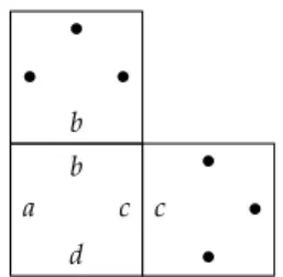
•(d,d^′)∈Vif the top colour ofdis equal to the bottom colour ofd^′ (see Figure 1.1).

AtilingofN×^NbyDis a functiont:N×^N→Dsuch that for allx,y∈^N

•(t(x,y),t(x+1,y))∈Hand

•(t(x,y),t(x,y+1))∈V.

A periodic tiling ofN×^NbyDis a tilingtfor which there exist two integersh,v ∈^N such thatt(x,y) = t(x+h,y) = t(x,y+v) for all x,y∈^N.

1.3 Domino problems

The decision problem DOMINO is described as DOMINO :={D: there exists a tiling ofN×^NbyD}

a b

c d

c

•

• b

Figure 1.1.Domino adjacency condition

Theorem 1.26(Berger, Robinson).DOMINO is co-r.e. and undecidable.

In this general form, this is quite a difficult result. A simpler variant is the so-called origin-constrained domino problem, that requires that a specific domino must be placed at the point(0, 0). With this requirement, it is straightforward to encode Turing machine computations by domino tilings (successive rows of the tiling correspond to successive configurations in the computation), and thus to reduce halting problems to tiling problems for domino systems. The origin constraint is used to encode the beginning of the computation (and to avoid that the entire space can be tiled by a domino corresponding to the blank symbol) Without an origin constraint, the problem is more difficult to handle; an essential part of the proof is the construction of a set of dominoes that admits only non-periodic tilings.

There are several extensions and variations of this result.

Theorem 1.27.A domino systemDadmits a tiling ofZ×^Zif, and only if, it admits a tiling ofN×^N.

Proof. It is clear that a tiling ofZ×^Zalso gives a tiling ofN×^N. The converse is a nice application of König’s Lemma. Suppose thattis a tiling ofN×^NbyD. There exists at least one dominodsuch that for alln there existi,j>nwitht(i,j) =d. Fix such ad. Further, for everyk∈^N, letS_kbe the square{−k, . . . ,−1, 0, 1, . . . ,k} × {−k, . . . ,−1, 0, 1, . . . ,k}.

(11)

We define a finitely branching tree whose nodes are the correct tilingst_kofS_kbyDsuch thatt_k(0, 0) =d. The root is the unique such tiling ofS0and the children of a tilingtkare the possible extensions to tilingst_k+1ofS_k+1. This tree contains paths of any finite length. By König’s Lemma it also contains an infinite path from the root, which

means thatDadmits a tiling ofZ×^Z. q.e.d.

The undecidability result from Theorem 1.26 can be strengthened to a recursive inseparability result.

Theorem 1.28.The set of domino systems admitting a periodic tiling ofN×^N, those that admit no tiling ofN×^Nand those that admit a tiling but not a periodic one are pairwise recursively inseparable.

The proof of Theorem 1.28 reduces the halting problemsH_ε⁺,H_ε⁻,H^∞_ε, to the domino problems. There exists a recursive function that associates with every TMMa domino systemDsatisfying

• IfM∈H⁺_ε thenDadmits a periodic tiling ofN×^N.

• IfM∈H⁻_ε thenDadmits no tiling ofN×^N.

• IfM∈H^∞_ε thenDadmits a tiling ofN×^Nbut no periodic one.

Definition 1.29.A computable functionfis aconservative reduction from domino systems to Xif, for all domino systemsD, f(D) =φ_Dis inXand the following holds:

•Dadmits a periodic tiling ofN×^N⇒ψ_Dhas a finite model

•Dadmits no tiling ofN×^N⇒ψ_Dis unsatisfiable

•Dadmits a tiling ofN×^Nbut no periodic one⇒ψ_Dis an infinity axiom.

Proposition 1.30. LetX∈FO. If there exists a conservative reduction from domino systems toXthenXis a conservative reduction class.

Proof. SinceFin-Sat(FO)andNon-Sat(FO)are recursively enumerable andInf-Axioms(FO)is co-recursively enumerable, we can associate with every first-order formulaψa Turing machineMsuch that

•ψ∈Fin-Sat(FO)⇒ρ(M)∈H⁺_ε,

•ψ∈Non-Sat(FO)⇒ρ(M)∈H⁻_ε,

1.4 Applications of the domino method

•ψ∈Inf-Axioms(FO)⇒ρ(M)∈H_ε^∞.

According to the assumption, there is a reductionD 7→φ_Dfrom domino systems toX. Thus, the domino method yields a conservative reduction from FO toX.

q.e.d.

1.4 Applications of the domino method

We now apply the domino method to obtain several reduction classes.

The Kahr-Moore-Wang class KMW is the class of all first-order sentences of form∀x∃y∀zφ, whereφis a quantifier-free formula without equality, whose vocabulary contains only binary relation symbols.

Theorem 1.31. The Kahr-Moore-Wang class is a conservative reduction class.

Proof. It suffices to construct a conservative reduction from domino systems to KMW, i.e., a mappingD 7→ψ_Dover a vocabulary consisting of binary relation symbols(P_d)_d∈Dsuch that

(1)Dadmits a periodic tiling ofN×^N⇒ψ_Dhas a finite model (2)Dadmits no tiling ofN×^N⇒ψ_Dis unsatisfiable

(3)Dadmits a tiling ofN×^Nbut no periodic one⇒^ψDis an infinity axiom

For a tilingt:N×^N→ D, an intended model ofψ_DisNwith the interpretationP_d={(i,j)∈^N×^N:t(i,j) =d}for alld∈D. We defineψ_Dby

ψ_D:=∀x∃y∀z _^

d̸=d^′

Pdxz→ ¬Pd^′xz

∧ ^_

(d,d^′)∈H

(P_dxz∧P_d′yz)∧ ^_

(d,d^′)∈V

(P_dzx∧P_d′zy). Obviouslyψ_Dis of the desired format, i.e.ψ_D∈KMW.

(1) Suppose thatDadmits a periodic tilingtofN×^N, such that t(x,y) =t(x+h,y) =t(x,y+v)for allx,y. We construct a finite model

(12)

ofψ_Das follows. Letm:=lcm(h,v)be the least common multiple ofh andv. Thentinduces a tiling

t^′:Z/mZ×^Z/mZ→D

witht^′(x,y) =t(x( modm),y( modm)).

It follows thatA= (Z/mZ,(P_d)_d∈D)withP_d={(i,j):t^′(i,j) =d} is a finite model forψ_D(forxinZ/mZchoosey:=x+1 (modm)).

(2) By analogous arguments, it follows, that wheneverDadmits a tiling ofN×^N, thenψ_Dhas a model overN.

(3) Finally we prove that ifψ_Dhas a model, thenDadmits a tiling ofN×^N, and if that model is finite, we even obtain a periodic tiling.

Consider the Skolem normal formφ_Dofψ_D: φ_D:=∀x∀z(^{^}

d̸=d^′

Pdxz→ ¬Pd^′xz

∧ ^_

(d,d^′)∈H

(P_dxz∧P_d′f xz)∧ ^_

(d,d^′)∈V

(P_dzx∧P_d′z f x).

Ifψ_Dis satisfiable, then alsoφ_Dhas a modelB= (B,f,(Pd)_d∈D). Define a tilingt:N×^N→Das follows: choose anyb∈B, and for all i,j∈^N, sett(i,j):=dfor the uniqued∈Dsuch thatB|=P_d(fⁱb,f^jb). SinceB|=φ_D, it follows thattis a correct tiling.

Now suppose thatB|=φ_Dis finite.

• _f • f b· · · • f

Chooseb∈Bsuch that, for somen≥1, fⁿb=b. Then the defined

tilingtis periodic. q.e.d.

Corollary 1.32. FO³is a conservative reduction class.

Later we shall prove thatFO²has the FMP.

Consider now formula classesX⊆FO over functional vocabularies.

One can prove that FO(τ)is a conservative reduction class ifτcontains

• two unary functions or

1.4 Applications of the domino method

• one binary function.

This is even true for sentences of the form∀xφwhereφis quantifier-free.

We stablish, again via a conservative reduction from domino problems, a weaker result from which the above mentioned ones can be obtained by interpretation arguments (see exercises).

Theorem 1.33. The classF, consisting of all sentences ∀xφwhere φ is a quantifier-free formula whose vocabulary consists only of unary function symbols, is a conservative reduction classes.

Proof. We define a conservative reductionD= (D,H,V)7→ψ_Dwhere ψ_D∈ F has the vocabulary{f,g,(hd)_d_∈_D}where all function symbols are unary. The intended model isN×^Nwith successor functions f andg. The subformula∀x(f gx=g f x)ensures that the models ofψ_D contain a two-dimensional grid. The fact that a positionxis tiled by d∈Dis expressed by requiring thath_dx=x, i.e. thatxis a fixed point ofhd.

ψ_D:=∀x f gx=g f x∧ ^{^}

d̸=d^′

(h_dx=x→h_d′x̸=x)

∧ ^_

(d,d^′)∈H

(h_dx=x∧h_d′f x=f x)

∧ ^_

(d,d^′)∈V

(hdx=x∧hd^′gx=gx).

We claim that there exists a tilingt:N×^N→ Dif and only ifψ_D is satisfiable.

”⇒” Assume thattis a correct tiling. Construct the (intended) model A= (N×^N,f,g,(h_d)_d∈D)with

– f(i,j) = (i+1,j), –g(i,j) = (i,j+1), –hd(i,j)





= (i,j) ift(i,j) =d

̸

= (i,j) otherwise.

ClearlyA|=ψ_D.

(13)

”⇐” ConsiderB= (B,f,g,(h_d)_d∈D)|=ψ_D.

Choose an arbitraryb∈Band definet:N×^N→Dby t(i,j):=diffB|=h_dfⁱg^jb= fⁱg^jb.

Note that every point in Bis a fixed-point of exactly one of the functionshd, andtis well-defined and a a correct tiling. Further, if Bis finite, thenσis periodic, and thus the reduction is conservative.

q.e.d.

Exercise 1.1.Prove that the more restricted classF2⊆ Fconsisting of sentences inF that contain just two unary function symbols, is also a conservative reduction class.

Hint: Transform sentences ∀xφ with unary function symbols f₁, . . . ,fminto sentences∀xφ˜:=∀xφ[x/hx,f_i/hgⁱ]whereh,gare fresh unary function symbols.

1.5 The finite model property

We study the finite model property (FMP) for fragments of FO as a mean to show that these fragments are decidable, and also to better understand their expressive power and algorithmic complexity.

Recall that a classX⊆FO has thefinite model propertyifSat(X) = Fin-Sat(X). Since for any decidable classX,Fin-Sat(X)is r.e. andSat(X) is co-r.e., it follows thatSat(X)is decidable ifXhas the FMP. In many cases, the proof that a class has the finite model property provides a bound on the model’s cardinality, and thus a complexity bound for the satisfiability problem. To prove completeness for complexity classes we make use of a bounded variant of the domino problem.

We shall illustrate the power of this method by a few examples.

Definition 1.34.Theatomic k-typeofa1, . . . ,akinAis defined as atp_A(a1, . . . ,a_k):={γ(x1. . . ,x_k):γatomic formula or negated

atomic formula such thatA|=γ(a1, . . . ,ak)}.

1.5 The finite model property In the examples that we consider here, the structures contain unary or binary relations only. Hence, to describe a structure it suffices to define its universe and to specify the atomic 1-types and 2-types for all of its elements.

Example1.35. Let Abe the structure(A,E1, . . . ,Em)where theEiare binary relations. Then fora∈A:

atp_A(a) ={Eixx:A|=Eiaa} ∪ {¬Eixx:A|=¬Eiaa}.

Themonadic class(also called the Löwenheim class) is the class of first-order sentences over a vocabulary the contains only unary predicates.

Theorem 1.36. The monadic class has the FMP.

Proof. Let A = (A,P₁Â, . . . ,P_nÂ) |= φ where qr(φ) = m. For each sequence of bitsα=α₁. . .αn∈ {0, 1}ⁿwe defineP_αÂ=Q1∩Q2∩. . .∩Qn, whereQi=P_iÂifαi=1 andQi=A\P_iÂifαi=0. Notice that the sets P_αÂdefine a partition ofA, and thatαcompletely describes the atomic 1-type of anya∈P_αÂ.

We constructBby taking min(|P_α^A|,m)elements into eachP_α^B. Ob- serve thatBis completly specified in this way, withP_i^B=^S_α_|_α_i₌₁P_α^B).

We show thatA≡mBusing the Ehrenfeucht-Fraïssé Theorem.

The following is a winning strategy for Duplicator in the Ehrenfeucht-Fraïssé game withm moves on (A,B): Answer any element chosen by Spoiler by an element with the same atomic type in the other structure, respecting equalities and inequalities with previously chosen elements. Due to the construction it is certainly possible to do that formmoves, so Duplicator wins the game. HenceA≡mB, and

thereforeB|=φ. q.e.d.

From the proof we see that the constructed finite modelBis in fact a submodel of the arbitrary modelAthat we started with. Thus we have in fact established a stronger result than the finite model property, namely thefinite submodel propertyof the monadic class: every infinite model of a sentence in the monadic class has a finite substructure which is also a model of that sentence.

(14)

In general it need not be the case that classes with the FMP also have the finite submodel property.

1.6 The two-variable fragment of FO

We denote relational first-order logic overkvariables by FO^k, i.e.

FO^k:={φ∈FO :φrelational,φonly containskvariables}. We have shown that the Kahr-Moore-Wang class KMW, and hence also FO³, are conservative reduction classes. We now prove that FO²has the finite model property and is thus decidable. Note that FO^kformulae are not necessarily in prenex normal form. A further motivation for the study of FO²is that propositional modal logic can be viewed as a fragment of FO²(in fact ML can be proven to be precisely the bisimulation invariant fragment of FO²).

Before we proceed to prove the finite model property for FO², as a first step we establish a normal form for formulae in FO².

Lemma 1.37(Scott). For each sentenceψ ∈FO²one can construct in polynomial time a sentenceφ∈FO²of the form

φ:=∀x∀yα∧

^n i=1

∀x∃yβi

such that α,β₁, . . . ,β_n are quantifier free and such that ψ and φare satisfiable over the same universe. Moreover, we have|φ|= O(|ψ| · log|ψ|).

Proof. First of all, we can assume that formulaeφ∈FO²only contain unary and binary relation symbols. This is no restriction since relations of higher arity can be substituted by introducing new binary and unary relation symbols. For example, if R is a relation of arity three, one could add a unary relationRxand three binary relationsRx,x,y,Rx,y,x

andRx,y,yand replace each atomR(x,x,x)(orR(y,y,y)) by Rx(x)(or Rx(y)) and atoms asR(x,x,y)orR(x,y,x)byRx,x,y(x,y)andRx,y,x(x,y) respectively. By adding appropriate new subformulae one can ensure

1.6 The two-variable fragment ofFO that the semantics are preserved, i.e. that the newly introduced relations partition a ternary relation in the intended sense. For example we would introduce as a new subformula∀x(Rx(x)↔Rx,x,y(x,x)).

Withψcontaining at most binary relations, we iterate the following steps untilψhas the desired form. We choose a subformulaQyηofψ (Q∈ {∀,∃},ηquantifier free) and add a new unary relationR:

ψ^′ := ψ[Qyη/Rx] ψ 7→ ψ^′∧ ∀x(Rx↔Qyη).

Rcaptures thosexthat satisfyQyη. The resulting formulaφis not yet of the desired form, but it is equivalent to the following:

(a) ifQ=∃, then

φ≡ψ^′∧ ∀x∀y(η→Rx)∧ ∀x∃y(Rx→η) (b) else ifQ=∀, then

φ≡ψ^′∧ ∀x∀y(Rx→η)∧ ∀x∃y(η→Rx)

Now use that conjunctions of∀∀-formulae are equivalent to a∀∀-formula and obtainψ≡ ∀x∀yα∧^Vⁿ

i=1∀x∃yβ_i. q.e.d.

Theorem 1.38. FO²has the finite model property. In fact, every satisfiable formulaψ∈FO²has a model with at most 2^|ψ|elements.

Proof. The proof strategy is as follows: we start with a modelAofψand proceed by constructing a new modelBofψsuch that|B| ≤2^O⁽^|^ψ^|⁾. For the construction the following definitions will be essential.

An elementa∈Ais said to be aking ofAif its atomic 1-type is unique inA, i.e. if atp_A(b)̸=atp_A(a)for allb̸=a. We let

•K:={a∈A:ais a king ofA}be the set of kings ofA, and

•P:={atp_A(a):a∈A,a∈/K}be the set of atomic 1-types which are realized at least twice inA.

Since A |= ∀x∃yβi for i = 1, . . . ,n, there exist (Skolem) functions f1, . . . ,fn : A → Asuch thatA |= β_i(a,f_ia)for all a∈ A. Thecourt

(15)

ofAis defined as

C:=K∪ {fik:k∈K,i=1, . . . ,n}.

LetCbe the substructure ofAinduced by C. We construct a model B|=ψwith universeB=C∪(P× {1, . . . ,n} × {0, 1, 2}).

A C K

B

C K P

P P

To specifyBwe setB|C=Cand for all other elements we specify the 1- and 2-types (in this way fixingBon the remaining part). However,

(1) This must be done consistently:

• atp_A(b,b^′)and atp_A(b,b^′′)must agree on atp_A(b), and

•γ(x,y)∈atp_B(b,b^′)⇔ γ(y,x)∈atp_B(b^′,b). (2) Of course we have to ensure thatB|=ψ.

We illustrate the construction with the following example.

Example1.39. Consider the formulaψover the signatureτ={R,B}(red edges and blue edges).

ψ = ∃x(Rxx∧Bxx)

∧ ∀x∀y((Rxx∧Bxx∧Ryy∧Byy→x=y)

∧(Rxx∨Bxx)

∧(Rxy∧Ryx→x=y)

∧(Bxy∧Byx→x=y)

∧(Bxy∧x̸=y→Ryy))

∧ ∀x∃y(x̸=y∧(Rxx→Rxy)

∧ (Bxx→Bxy)).

1.6 The two-variable fragment ofFO LetA|=ψ, thenAlooks like follows:

• • • • · · ·

K C

In this caseP={{Rxx,¬Bxx},{¬Rxx,Bxx}}and the universe of BisB=C∪(P× {1} × {0, 1, 2}).

We proceed to constructBby specifying the 1-types and 2-types of its elements as follows.

(1) The atomic 1-types of elements(p,i,j)are set to atp_B((p,i,j)) =p.

(2) The atomic 2-types atp_B(b,b^′)will be set so thatB|=∀x∃yβ_ifor i=1, . . . ,m.

Choose for eachp∈Pan elementh(p)∈Awith atp_A(h(p)) =p.

Find for eachb ∈ Band eachia suitable element b^′ such that B|=β_i(b,b^′)(by defining atp_B(b,b^′)appropriately).

(a) Ifbis a king, setb^′:= fi(b)∈C⊆B. ThenB|=β_i(b,b^′). (b) Ifb∈C\K(non-royal member of the court), distinguish:

• If f_i(b)∈K, then setb^′:= f_i(b)∈K⊆B.

• Otherwise it holds that atp_A(fi(b)) =p∈P.

In this case, set b^′ := (p,i, 0). Now set atp_B(b,b^′) := atp_A(b,f_i(b)). ThusB|=β_i(b,b^′)sinceA|=β_i(b,f_i(b)). (c) Ifb= (p,j,ℓ)for somep ∈P,j∈ {1, . . . ,n},ℓ∈ {0, 1, 2}, let

a:=h(p)and considerf_i(a).

If fi(a)∈K, setb^′= fi(a)and atpB(b,b^′):=atpA(a,b^′). If fi(a)∈/K, then atp_A(fi(a)) =p^′∈P.

Setb^′:= (p^′,i,(ℓ+1) (mod 3)).

Then set atp_B(b,b^′):=atp_A(a,fi(a)), and thusB|=β_i(b,b^′). To complete the construction ofB, let b1,b2 ∈ B be such that atp_B(b1,b2)is not yet specified. Choosea1,a2∈Aso that

atp_A(a1) = atp_B(b1)and atp_A(a2) = atp_B(b2)

(16)

and set

atp_B(b1,b2):=atp_A(a1,a2). SinceA|=α(a1,a2), alsoB|=α(b1,b2).

For the previously considered example,Blooks as follows:

C K

P× {0} P× {1}

P× {2}

•

• Overall, we obtainB|=∀x∀yα∧^Vⁿ

i=1∀x∃yβ_i=ψ, and the size ofB is restricted by

|B|= |C|

≤|K||{z}(n+1)

+3n|P|=O(n·# (atomic 1-types)).

Forkrelation symbols, there are 2^katomic 1-types, hence|B|=2^O(|ψ|). q.e.d.

This result implies that Sat(FO²) is in NEXPTIME (indeed it is NEXPTIME-complete), since we can simply guess a finite structure Aof exponential size (in the length ofψ) and verify thatA|=ψ.

Corollary 1.40. Sat(FO²)∈NEXPTIME= (^S

kNTIME(2ⁿ^k)).

This is a typical complexity level for decidable fragments of FO.

In fact,Sat(FO²)is even complete for NEXPTIME. For showing this, we reduce a bounded version of the domino problem toSat(FO²). Definition 1.41. LetD = (D,H,V)be a domino system and letZ(t) denoteZ/tZ×^Z/tZ. For a wordw=w0, . . . ,wn−1∈Dⁿwe say that DtilesZ(t)with initial conditionwif there isτ:Z(t)→Dsuch that

1.6 The two-variable fragment ofFO

• ifτ(x,y) =dandτ(x+1,y) =d^′then(d,d^′)∈H for all(x,y)∈Z(t),

• ifτ(x,y) =d,τ(x,y+1) =d^′then(d,d^′)∈V for all(x,y)∈Z(t)and

•τ(i, 0) =wifor alli=0, . . . ,n−1.

LetDbe a domino system andT:N→^Na mapping. Define DOMINO(D,T):={w∈D^∗:DtilesZ(T(|w|))with initial

conditionw}. One can describe computations of a (in this case non-deterministic) Turing machine by domino tilings in such a way that the input condition of the domino problem relates to the initial configuration of the Turing machine. The restrictions on the size of the tiled rectangle correspond to the time and space restrictions of the Turing machine. To prove that a problem A is NEXPTIME-hard, it then suffices to show that DOMINO(D, 2ⁿ)≤pA.

Our goal is to show that DOMINO(D, 2ⁿ)reduces toSat(X)for relatively simple classesX⊆FO. Set

X={φ∈FO²:φ=∀x∀yα∧ ∀x∃yβ, s.t.α,βquantifier-free, without=, and with only monadic predicates}. We show that Sat(X) is NEXPTIME-complete and hence also Sat(FO²)is NEXPTIME-complete.

Lemma 1.42.For each domino system D = (D,H,V) there exists a polynomial time reductionw∈Dⁿ7→ψw∈Xsuch thatDtilesZ(2ⁿ) with initial conditionwif and only ifψwis satisfiable.

Proof. The intended model ofψwis a description of a tilingτ:Z(2ⁿ)→ Din the universeZ(2ⁿ).

Letz= (a,b)∈Z(2ⁿ)witha=ⁿ⁻¹∑

i=0ai2ⁱandb=ⁿ⁻¹∑

i=0bi2ⁱ. Encode the tuple as(ao, . . . ,an−1,b0, . . . ,bn−1)∈ {0, 1}²ⁿ.

To encode the tiling, we defineψwwith the monadic predicatesXi, X_i^∗,Y_i,Y_i^∗,N_ifor 0≤i<nandP_d(d∈D)with the following intended

(17)

meaning:

Xiz iff ai=1.

X_i^∗z iff a_j=1 for allj<i.

Yiz iff bj=1.

Y_i^∗z iff b_j=1 for allj<i.

Niz iff z= (i, 0). P_dz iff τ(z) =d.

ψw will have the formψw = ∀x∀yα∧ ∀x∃yβ, where βaccounts for the correct interpretation ofX_i,X_i^∗,Y_i,Y_i^∗,N_iand ensures that every element has a successor, andαaccounts for the description of a correct tiling.

Nowβis the the following formula:

β=X^∗₀x∧Y₀^∗x

∧

n−1^ i=1

X_i^∗x↔(X^∗_i−1x∧X_i−1x)

∧

n−1^ i=1

Y_i^∗x↔(Y_i−1^∗ x∧Y_i−1x)

∧

n−1^ i=0

Xiy↔(Xix⊕X^∗_ix)

∧

n−1^ i=0

Yiy↔(Yix⊕(Y_i^∗x∧Xn−1x∧X^∗_n−1x))

∧ N0x↔(

n−1^ i=0

¬Xix∧ ¬Yix)

∧

n−1^ i=0

Nix↔Ni+1y.

We define the following shorthands for use inα:

H(x,y) :=

n^−1 i=0

(Y_iy↔Y_ix)∧

n^−1 i=0

(X_iy↔(X_ix⊕X_i^∗x))

1.6 The two-variable fragment ofFO

V(x,y) :=

n^−1 i=0

(X_iy↔X_ix)∧

n^−1 i=0

(Y_iy↔(Y_ix⊕Y_i^∗x)). Nowαis defined to be

α= ^{^}

d̸=d^′

¬(P_dx∧P_d′x)

∧ (H(x,y)→ ^_

(d,d^′)∈H

(Pdx∧Pd^′y))

∧ (V(x,y)→ ^_

(d,d^′)∈V

(Pdx∧P_d′y))

∧ (

n^−1 i=i

(Nix→Pwix)).

Claim1.43. ψw is satisfiable if and only if D tiles Z(2ⁿ) with initial conditionw.

Proof. We show both directions.

(⇐) Consider the intended model,ψwholds in it.

(⇒) ConsiderC= (C,X1, . . .)|=ψ_wand define a mapping f: C →Z(2ⁿ)

c 7→(a,b)≡(a0, . . . ,an−1,b0, . . . ,bn−1)

witha_i=1 iff C|=X_ic and bi=1 iff C|=Yic.

AsC|=∀x∃yβ,fis surjective. Choose for eachz∈Z(2ⁿ)an element c∈f⁻¹(z)and setτ(z) =dfor the uniquedthat satisfiesC|=Pdc.

Thenτis a correct tiling with initial conditionw. q.e.d.

Since the length ofψwis|ψw|=O(nlogn), the above claim com-

pletes the proof of the lemma. q.e.d.

1 The classical decision problem

Algorithmic Model Theory SS 2016

Prof. Dr. Erich Grädel and Dr. Wied Pakusa

c b n d

Contents

1 The classical decision problem

1.1 Basic notions on decidability

1.2 Trakhtenbrot’s Theorem

1.3 Domino problems

1.4 Applications of the domino method

1.5 The finite model property

1.6 The two-variable fragment of FO