Notes on Thermodynamic Formalism.

Notes on Thermodynamic Formalism.

H. Bruin October 5, 2017

Abstract

1 Historic Background

The program of statistical physics started with the aim of understanding how the mi- croscopic considerations (say, the mechanics of single molecules) lead to macroscopic observations of the whole system. In particular, but not exclusively, the behaviour of an ideal gas (a liter of which roughly contains 2.7·10²² molecules, cf. to the ≈2.710²⁶ (the number of Avogadro) in a mol of substance.

• The macroscopic and experimental theory of the time included measurements of temperature, pressure, energy, etc. How should they be understood as averages over the movements of all the single particles? One is helped by conservation laws, such as the First Law of Thermodynamics:

U =Q−W energy flow = heat flow minus net work done.

• What exactly is entropy, i.e.,the measure of disorder of the system. It appears in the Second Law of Thermodynamics:

dQ=T dS heat transfer = temperature times change of entropy and the Third Law of Thermodynamics:

the entropy of a perfect crystal at zero temperature is zero, but how to define such a quantity mathematically?

• Explain the macroscopic laws of thermodynamics, especially:

– Systems strive towards lowest energy.

– Systems strive towards largest entropy.

Especially the last was not without controversy: Newtonian reversibility doesn’t reconcile with increase of entropy. Apart from this, there is Gibbs’ paradox:

Imagine a container divided into two parts A and B, which do communicate.

The parts A and B are filled randomly with gases g_A and g_B. If g_A and g_B are different, the entropy increases by the mixture of the gases. If g_A and g_B are the same gas, then entropy is already maximal.

• Description of phase transitions:

solid ↔ liquid ↔ gaseous magnetized ↔ non-magnetized

super-conductive ↔ conductive ↔ non-conductive Some of the protagonists of this theory are the following:

• James Clark Maxwell (1831 - 1879). Although his work of electromagnetism and color theory is much better known, he did publish works of kinetic theory of gas and also the “molecular” structure of conductors.

• Ludwig Boltzmann (1844 - 1906). He is basically the founder of this theory, but his ideas met with a lot of criticism. This was in a time when the existence of atoms was still a hypothesis rather than a fact. His theory didn’t match empiri- cal observations, and didn’t yet fully explain the problems with entropy increase.

Boltzmann moved between universities a lot (Graz, Vienna, Leipzig), being usu- ally very unhappy if he shared his working place with scientific adversaries (e.g.

Mach in Vienna, Oswald in Leipzig). Nonetheless he had success; for instance, his lectures on natural philosophy were so popular that the largest lecture hall in Vienna at the time wasn’t big enough, and he had to move his lectures to a hall in the imperial palace.

• Josiah Willard Gibbs (1839 - 1903). Gibbs was the first to include probability theory in his analysis, and may be credited with coining the word “statistical mechanics”. He published only late in his life. His 1902 book on the subject was praised by its mathematical rigor and elegance, but sometimes criticised for not really addressing the physical-philosophical problems of the structure of gases.

• Henri Poincar´e (1854 - 1912). His theorem (now called Poincar´e recurrence) gave a mathematical refutation of the principle of ever increasing entropy.

• Albert Einstein (1879 - 1955). Between 1902 to 1904, Einstein published sev- eral papers on statistical mechanics, which were definitely helpful in his treatise

of Brownian motion and of the photo-electric effect (1905), for which he would eventually receive the Nobel prize (i.e.,not for his relativity theory!).

• Paul and Tatiana Ehrenfest (1880 - 1933 and 1876 - 1964) published in 1910 an influential paper on the subject, in which they made the state of the art of the time accessible to a wide (German-speaking) audience. Among other things, they gave a more modest and mathematcally sound version of Boltzmann’s famous but unrealistic Ergoden Hypothese.

• George Birkhoff (1884 – 1944) proved in 1931 the pointwise version of the Ergodic Theorem which was long anticipated, and was crucial for the development of the mathematical side of thermodynamic formalism.

• John von Neumann (1903 – 1957) proved theL^p version of the Ergodic Theorem.

His result came before Birkhoff’s but was published slightly later (in 1932). In this struggle for priority, Birkhoff was not entirely innocent.

• Wilhelm Lenz (1988 - 1957) was PhD supervisor of Ising (below), and suggested a now famous model of ferro-magnetism to Ising.

• Ernst Ising (1900 - 1998) treated this system in his thesis, found no “phase transi- tions” and but concluded that the model was insufficient to explain the magneti- zation of iron. He was in fact quite surprised to learn that 25 years after his thesis, people were still interested. In fact, the model doesn’t explain magnetization in a one-dimensional model, but performs much better in dimension three.

• Andrej Kolmogorov (1903-1987), Russian probabilist and founding father of er- godic theory in Russia. His definiton of entropy paved the way for the current mathematical approach to thermodynamic formalism.

The introduction of thermodynamic formalism within the mathematical field of dynam- ical systems occurred in the 1970s, and was primarily due to the following people.

• Yakov Sina˘ı(1935 -): Mathematical physicists in moscow and Princeton, student of Kolmogorov. He proved the ergodicity of what is now called Sinai billiards, which is a model for bounding molecules in a gas.

• David Ruelle (1935 -): Mathematical physicists born in Belgium but worked mostly in France, mainly on statistical physics and turbulence. The Ruelle-Takens route to chaos, Ruelle’sζ-function and the Ruelle inequality are named after him.

• Rufus Bowen (1947 - 1978): Mathematician at Berkeley (USA), student of Field’s medalist Stephen Smale, worked on Axiom A diffeomorphisms and symbolic dy- namics.

1.1 Introductory example of the Ising model

This extended example is meant to give a feel for many of the ingredients in thermody- namic formalism. It is centred around a simplified Ising model, which can be computed completely.

We take the configuration space Ω = {−1,+1}^Z, that is the space of all bi-infinite sequences of +1’s and−1’s. This give a rough model of ferro-magnetic atoms arranged on a line, having spin either upwards (+1) or downwards (−1). If all spins are upwards (or all downwards), then the material is fully magnetized, but usually the heat in the material means that atom rotate directing their spin in all directions over time, which we discretize to either up or down.

Of course, infinitely many atoms is unrealistic, and hence a configuration space{−1,+1}^[−n,n]

would be better (where [−n, n] is our notation of the integer interval{−n,−n+1, . . . , n−

1, n}), but for simplicity, let us look at the infinite line for the moment.

A probability measure µindicates how likely it is to find a particular configuration, or rather a particular ensemble of configurations. For example, the fully magnetized states are expressed by the measures:

δ+(A) =

1 if A3(. . . ,+1,+1,+1,+1, . . .) 0 if A63(. . . ,+1,+1,+1,+1, . . .)

and δ− with the analogous definition. For these two measures, only one configuration is likely to occur. Usually a single configuration occurs with probability zero, and we have to look at ensembles instead. Define cylinder sets

C_m,n(ω) = {ω⁰ ∈Ω :ω⁰_i =ω_i for i∈[m, n]}

as the set of all configurations that agree with configuration ω on sitesifor m6i6n.

Its length is n−m+ 1. Another notation would be C_m,n(ω) = [ω_mω_m+1. . . ω_n].

The Bernoulli measure (stationary product measure) µp is defined as¹ µp([ωmωm+1. . . ωn]) =

n

Y

i=m

p(ωi), wherep(+1) =p and p(−1) = 1−p.

There is a Bernoulli measure µ_p for each p ∈ [0,1] and µ₁ = δ₊, µ₀ = δ−. However, for p ∈ (0,1), every single configuration has measure 0. The Law of Large Numbers implies that the set of configurations in which the frequency of +1’s is anything else than p has zero measure.

Since physical problem is translation invariant. Define the left-shift as σ(ω)_i =ω_i+1.

1This measure extends uniquely to all measurable sets by Kolmogorov’s Extension Theorem.

Translation invariance of a measure then means shift-invariance: µ(A) = µ(σ(A)) for each ensemble A ⊂ Ω. Many probability measures on Ω are not translation invariant, but fortunately, the examples µ_p above are.

Another example of shift-invariant measures are the Gibbs measures, associated to some potential function ψ : Ω →R; the integral R

Ωψ dµ is called the (potential)energy of µ.

Definition 1. A measure µ is a Gibbs measure w.r.t. potential function ψ : Ω→R if there are constants C > 0 and P ∈ R such that for all cylinder sets C_m,n and all ω ∈C_m,n,

1

C 6 µ(C_m,n) expPn

i=m(ψ◦σⁱ(ω)−P) 6C. (1)

The numberP is called the pressure; in this setting it is a sort of normalizing constant, adjusting the exponential decrease of the denominator to the exponential decrease of the numerator²

If we choose the potential to be ψ(ω) =

logp if ω₀ = +1 log 1−p if ω₀ =−1 ,

then the Bernoulli measure µ_p is actually a Gibbs measure, with pressure P = 0 and

“distortion constant”C = 1. Indeed, µ(C_m,n(ω)) =

n

Y

i=m

p(ω_i) =

n

Y

i=m

e^ψ(σi(ω))= exp(

n

X

i=m

ψ(σⁱ(ω))), and (1) follows.

The next ingredient is entropy. We postpone the precise definition, except for to say that there are different kinds. The system itself can havetopological entropyh_top(σ) which is independent of the measure, while each shift-invariant measureµhas its metric entropy or rather measure theoretical entropy h_µ(σ). For the Bernoulli measure µ_p, the measure theoretical entropy is

h_µp(σ) =−(plogp+ (1−p) log(1−p)) is the minus the expectation of ψ.

Exercise 1. For ϕ: [0,1] → R defined as ϕ(x) = −(xlogx+ (1−x) log(1−x)), we can write h_µp(σ) =ϕ(p). Compute the limits limx→0ϕ(x) and limx→1ϕ(x). Conclude that δ₊ and δ₋ have zero entropy. (This agrees with the idea that entropy is suppose to measure disorder.) Where does ϕ assume its maximum? What does this suggest about the measure of maximal entropy?

2This is the definition for one-dimensional lattices. For ad-dimensional lattice, we need to add an extra factor (n−m+ 1)^d−1in the lower and upper bounds in (1).

Exercise 2. Compute its first and second derivative. Is ϕ (strictly) concave?

Let us fix the potential

ψ(ω) =

0 if ω0 = +1

1 if ω₀ =−1. (2)

The potential energy E(µ) = R

Ωψ dµ becomes smaller for measures that favours con- figurations ω where many entries are +1. We can think of ψ as representing a fixed external magnetic field; the better the atoms align themselves to this field, the smaller the potential energy of their configuration. In extremo, E(δ+) = 0, but the entropy of δ₊ is zero, so we don’t maximise entropy with this choice.

Pressure can also be defined by the Variational Principle. We introduce a weighing parameter β ∈ R between energy and entropy content of the measure. The physical interpretation of β = 1/T, where T stands for the absolute temperature (i.e., degrees Kelvin normalised in some way), and thus it makes only physical sense to take β ∈ (0,∞), but we will frequently look at limit case β →0 andβ → ∞.

Now let the (Variational) Pressure be P(β) = sup{h_µ(σ)−β

Z

ψ dµ : µ is a shift-invariant probability measure} (3) A shift-invariant probability measure µ is called equilibrium state or equilibrium measure, if it assume the pressure in (3).

For the limit case T → ∞, i.e., β → 0, the potential energy plays no role, and we are just maximising entropy. For the limit case T →0, i.e., β → ∞, the potential energy becomes all important, so in our example we expectδ₊to be the limit equilibrium state.

The physical interpretation of this statement is: as the temperature decreases to zero for some fixed external magnetic field (and also as the external magnetic field grows to infinity), the material becomes totally magnetized.

The question is now: do we find total magnetization (i.e.,the measureδ₊as equilibrium state) also for some positive temperature (or finite external magnetic field)?

For each fixed measure, the functionβ 7→hµ(σ) +βR

ψ dµis a straight line with slope

−R

ψ dµ (non-positive because our potential ψ is non-negative) and abscissa h_µ(σ). If we look at (3) again, we can view the pressure function β 7→ P(β) as the envelope of all these straight lines. From this it follows immediately that β 7→ P(β) is continuous and convex (and non-increasing due toψ being non-negative).

Once full magnetization is obtained, increasingβfurther will not change the equilibrium state anymore. Indeed, there is no measure that favours ω_i = +1 more than δ₊. So if there is a finite β₀ such that δ₊ is equilibrium state, then P(β) = 0 for allβ >β₀. We can call this a freezing phase transition, because at this parameter, the equilibrium state doesn’t change anymore (as if the system is frozen in one configuration). The

right-hand slope of the pressure function at β₀ is 0; how abrupt thisphase transition is depends also on the left slope at β₀ which might be different from 0, but always >0 because of convexity.

Let us now do the computation if there really is a phase transition at a finite β0. For simplicity (and without justification at the moment) we will only compute the supremum in (3) over the Bernoulli measures µ_p. So then (3) simplifies to

P(β) = sup

p∈[0,1]

−(plogp+ (1−p) log(1−p))−β(1−p) =: sup

p∈[0,1]

F(µ_p, β)

The quantity F(µ_p, β) is called the free energy of the measure µ_p. In our simplified case, it is a smooth curve in p, so to find the supremum (= maximum), we simply compute the derivative and put it equal to 0:

0 = ∂

∂pF(µ_p, β) =−(logp−log(1−p)) +β.

This is equivalent to log_1−p^p =β, i.e., p= e^β

1 +e^β, 1−p= 1 1 +e^β Substituting in P(β), we find that the pressure is

P(β) = − e^β

1 +e^β log e^β

1 +e^β + 1

1 +e^β log 1 1 +e^β

−β 1 1 +e^β

= − e^β + 1

1 +e^β log e^β 1 +e^β

| {z }

+ 1

1 +e^β log 1

1 +e^β − 1

1 +e^β log e^β 1 +e^β

| {z }

!

−β 1 1 +e^β

= −

log e^β

1 +e^β − β

1 +e^β

− β 1 +e^β

= log(1 +e^−β)







→0 asβ → ∞

= log 2 if β = 0

∼ −β asβ → −∞

So the pressure function is smooth (even real analytic) and never reaches the lineβ ≡0 for any finite β. Hence, there is no phase transition.

Exercise 3. Verify that for potential (2),µ_p is indeed a Gibbs measure. For which value of the pressure? Here it is important to incorporate the factor −β in the potential, so ψβ(ω) = 0 if ω0 = 1 and ψβ(ω) =−β if ω0 =−1.

In the proper Ising model, the potential also contains also a local interaction term between nearest neighbors:

ψ(ω) =X

i

J ω_iω_i+1+ψ_ext(ω),

whereJ <0, so neighboring atomic magnets with the same spin have lower joint energy than neighboring atoms with opposite spin. The termψ_ext(ω) still stands for the exter- nal magnetic field, and can be taken as ψ in (2). This gives a problem for the infinite lattice, because here all configurations have a divergent sum P

iJ ω_iω_i+1. Ising’s solu- tion to this problem lies in first dealing with a large lattice [−n, n], so the configuration space is {−1,+1}^[−n,n], and considering the Gibbs measures and/or equilibrium states projected to fixed finite lattice [−m, m] (these projections are called marginal mea- sures), and then letting n tend to infinity. Such limits are called thermodynamic limits. If there is no external magnetic field (i.e.,ψ_ext≡0), then as β → ∞, n→ ∞, there are two ergodic thermodynamic limits, namely δ₊ andδ−. There is no preference from one over the other; this preference would arise if the is an external magnetic field of definite direction. However, no such magnetization takes place for a finiteβ. For this reason, Ising dismissed the model as a good explanation for magnetization of iron (and other substances). However, as was found much later, on higher dimensional lattices, the Ising model does produce phase transitions and magnetization at finite values ofβ (i.e.,positive temperature).

2 Configuration Spaces, Subshifts of Finite Type and Symbolic Dynamics

In this section we provide some examples of frequently occurring configuration spaces, and we want to give an indication of their size, which is directly related to the complexity of the maps we define on them. We start with symbolic spaces, which may seem the most abstract, but which are used to code dynamics on more concrete space symbolically.

2.1 Symbolic spaces

LetA ={0, . . . , N −1} be some finite collection of symbols, called the alphabet. We can make finite words of these symbols by concatenation; the notation of the collection of these finite words is A^∗. More interesting are the infinite words of symbols, A^N0 or A^Z, depending on we have one-sided (with N⁰ = {0,1,2,3, . . .}) or two-sided infinite words. If Ω =A^N0 orA^Z, then we can define the left-shift σ : Ω→Ω as

σ(ω)_i =ω_i+1 for all i∈N orZ.

The space (Ω, σ) is called the one-sided and two-sided full shift on n letters. The left-shift is invertible (and σ⁻¹ is the right-shift) on two-sided infinite words, i.e., on Ω =A^Z. Define a metric on Ω as

d(ω, ω⁰) =X

n

2^−|n|(1−δ(ω_n, ω_n⁰)), where the Dirac deltaδ(a, b) =

1 if a=b 0 if a6=b

In this metric, two words ω and ω⁰ are close together if they agree on a large block around the zero-th coordinate.

Exercise 4. Show that in the above topology, Ωis a Cantor set. That is: Ωis compact, has no isolated points and is totally disconnected (each of its connected components is a point).

Exercise 5. There is nothing special about the number 2. We could take any λ > 1 instead, obtaining a metric

d_λ(ω, ω⁰) =X

n

λ^−|n|(1−δ(ω_n, ω⁰_n)).

Show that the metricsdandd_λ are not equivalent in the sense that there would beC > 0 so that

1

Cd(ω, ω⁰)6dλ(ω, ω⁰)6Cd(ω, ω⁰).

On the other hand, show that the identity mapI : (Ω, d)→(Ω, d_λ) is uniformly contin- uous, with uniformly continuous inverse.

Exercise 6. Take λ >2 and show that the identity map I : (Ω, d)→(Ω, dλ) is H¨older continuous, i.e., there are C and exponent α such that

d_λ(ω, ω⁰)6Cd(ω, ω⁰)^α. What is the largest value of α that we can take?

Definition 2. A set Σ⊂Ω is called a subshift if it is closed and shift-invariant, i.e., σ(Σ)⊂Σ.

The prime example of a subshift are the subshifts of finite type (SFT)in which the occurrence of a finite collection of words is forbidden. For example, the Fibonacci SFT

Σ¬11={ω ∈ {0,1}^N or {0,1}^Z : ω_iω_i+1 6= 11 for all i}.

Naturally, we can think of SFTs in which blocks of length >2 are forbidden, but since there are only finitely many forbidden word, we can always recode the subshift (using a larger alphabet) so as to obtain a SFT in which only some words of length 2 are forbidden. This means that we can define a transition matrix:

A= (a_i,j)^N−1_i,j=0 a_i,j =

1 if the word ij is allowed, 0 if the word ij is forbidden.

For example, the transition matrix of Σ_¬11is 1 1

1 0

. The transition matrixAis a non- negative matrix, and hence (by the Perron-Frobenius Theorem) has a real eigenvalue ρ(A) which is at least as large as any other eigenvalue of A. In fact, if A is irreducible and a-periodic (that is, there is n₀ ∈N such that Aⁿ is a strictly positive matrix for all n>n0), then ρ(A) has multiplicity one and is strictly larger than the absolute value of every other eigenvalue.

Exercise 7. Examine the eigenvalues of 1 0

0 1

and

0 1 1 0

to see what lack of irreducibility and of non-periodicity can mean.

Exercise 8. Recode the SFT Σ¬101,111 to a SFT with forbidden words of length 2 only.

Compute the corresponding transition matrix.

Example 1. One can consider configuration spaces over higher-diemnsional lattices, for instance

Ω ={−1,+1}^Z2

for which every ω ∈ Ω is an infinite square patterns of −1’s and +1s. There are now two shifts, the left-shift σ with σ⁻¹ being the right-shift, but also the down-shift τ with τ⁻¹ being the up-shift, and τ◦σ =σ◦τ. Also here you can consider subshifts of finite type, for instance Σ_¬11,1

1

would stand for all infinite square patterns of −1’s and +1s without two+1s begin left-right or up-down neighbors, but diagonal neighbors is allowed.

In this case, the word-complexity p(m, n), here the number of different patterns in an m×n-block, is an open problem. We don’t know the precise value of lim_nn¹ logp(n, n).

2.2 Sizes of symbolic spaces

Recall that cylinder sets of length n−m+ 1 are

Cm,n(ω) = [ωmωm+1. . . ωn] ={ω⁰ ∈Ω :ω_i⁰ =ωi for i∈[m, n]}

as the set of all configurations that agree with configuration ω on sites i for m 6 i 6 n. If Ω is a one-sided shift-space, then it is convenient to abbreviate n-cylinders as C_n(ω) = [ω₀. . . ωn−1].

Definition 3. The word-complexity of a subshift Σ is defined as p(n) =p(n,Σ) = #{different n-cylinders in Σ}.

Clearly p(n) = Nⁿ for the full-shift on N letters. For the Fibonacci shift Σ¬11 on two letters we have

p(1) = 2, p(2) = 3, p(3) = 5, . . . , p(n) is n+ 1st Fibonacci number.

To see why this is true, let p0(n) be the number of n-cylinders ending with 0 andp0(n) be the number of n-cylinders ending with 1. Then p₁(n) =p₀(n−1), because every 1 must have been precede by a 0. On the other hand, p₀(n) = p₁(n−1) +p₀(n−1) = p0(n−2) +p0(n−1). With initial valuesp0(1) = 1 andp0(2) = 2, it follows immediately that p₀(n) is the n-th Fibonacci number. The step to p(n) is now easy.

Theorem 1. For a SFT with transition matrix A,

n→∞lim 1

nlogp(n) = logρ(A)

is the logarithm of the largest (Perron-Frobenius) eigenvalue of A.

Proof. Matrix multiplication Aⁿ = (aⁿ_i,j)^N−1_i,j=0 gives the number of allowed words of length n + 1 that start with i and end with j. Hence the total number of words of lengthn+1 isPN−1

i,j=0aⁿ_i,j, but the latter grows asρ(A)ⁿ(disregarding polynomial factors if the Jordan block associated to ρ(A) is non-trivial). Therefore lim_n→∞ ¹_nlogp(n) = limn→∞ 1

nlogρ(A)ⁿ= logρ(A), as required.

2.3 Further configuration spaces

In this subsection, we review some configuration spaces and maps acting on them that frequently occur in thermodynamic formalism an dynamics as a whole. Without a physical interpretation as direct, maybe, as {−1,+1}^Z as the simple Ising model of Section 1, it is quite common within mathematics to use manifolds as configuration space Ω. In this setting, the word “configuration” seems less apt, so we tend to prefer the wordphase spaceinstead, even though this has nothing to do with phase transition in physics. Maybedynamical spacewould yet be better, but that is not used so often, in fact only to distinguish it from parameter space.

Examples of phase spaces are: the unit interval [0,1], the unit circle S¹ = R/Z, the d-dimensional torus T^d =R^d/Z^d, the d-dimensional sphere S^d, etc. In this case, there is no shift, but we have to specify the dynamics f : Ω → Ω explicitly, and it doesn’t express translation invariance anymore.

Example 2. An example is the angle doubling map T₂ :S¹ →S¹, defined as T2(x) = 2x (mod 1),

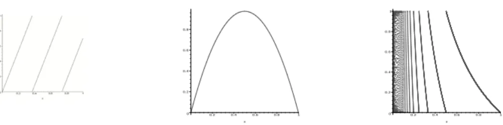
and the generalization T_d(x) =dx (mod 1) for anyd∈Zis easy to grasp. In fact, there is no reason to stick to integer d; we can define the β-transformation (see Figure 1) for any β ∈R as

T_β(x) = βx (mod 1).

This is not continuous anymore for non-integer β, taking away the advantage of the circle S¹. Therefore, the β transformation is usually defined on the unit interval: T_β : [0,1]→[0,1].

Example 3. The rotation map R_γ :S¹ →S¹ is defined as R_γ(x) = x+γ (mod 1),

0 0.2 0.4 0.6 0.8

0.2 0.4 0.6 0.8 1

x

0 0.2 0.4 0.6 0.8 1

0.2 0.4 0.6 0.8 1

x

Figure 1: The β-transformation (β = 2.7), quadratic Chebyshev map and Gauss map.

and depending on whether the rotation angle γ is rational or not, every orbit is periodic or dense. One can easily construct higher dimensional analogs,i.e.,rotations R_~γ :T^d→ T^d with a d-dimensional rotation vector.

Example 4. The integer matrix A =

2 1 1 1

acts as a linear transformation on R², with eigenvalues λ± = ^3±

√ 5

2 and eigenvectors ~v± =

_1±^√₅

2

1

. It preserves the integer lattice Z², so it is possible to defined the factor map f :T² =R²/Z² →T² as

f x

y

= 2 1

1 1 x y

(mod 1).

This is called Arnol’d cat-map because Arnol’d in his book [2, 3] uses a picture of a cat’s head to show what happens to shapes when iterated by f. The tangent space T_p of the fixed point p =

0 0

(and in fact near every point), decomposes in an unstable direction E^u(p) = span~v₊ and a stable direction E^s(p) = span~v−. This means that shapes are stretched by a factorλ₊ in the~v₊-direction and contracted by a factorλ− in the~v−-direction. But since λ+·λ− = 1, the area doesn’t change under f.

Definition 4. A map f on a d-dimensional manifold M is called Anosovif

• At each p ∈ M, there is a splitting of the tangent space T_pM = E^u(p)⊕E^s(p) which is invariant under the derivative map: Df_p(E^u/s(p)) =E^u/s(f(p)).

• The splitting E^u(p)⊕E^s(p) depends continuously on the point p.

• There is exponential expansion and contraction along E^u/s(p), i.e., there is λ >1 and C >0 such that

kDf_pⁿ·vk > Cλⁿkvk for all v ∈E^u and p∈M; kDf_pⁿ·vk 6 1

Cλ⁻ⁿkvk for all v ∈E^s and p∈M.

2.4 Symbolic dynamics

In this section we make the connection between dynamics on manifolds and symbolic spaces. The latter is a coded version of the first. For this coding, we need a partition P = (X_n) of the phase space X, and each partition element has X_n a label, which is a letter from the alphabet A. The orbit orb(x) = (f^k(x)) is associated to a code i(x) =i₀(x)i₂(x). . . (or i(x) = . . . i₋₁(x)i₀(x)i₂(x). . . if f is invertible) defined as

i_k(x) =n if f^k(x)∈X_n. (4)

The coding map or itinerary map i : X → Ω = A^N0 or A^Z need not be injective or continuous, but hopefully, the points where i fails to be injective or continuous are so small as to be negligible in terms of the measures we are considering, see Section 3.

The following commuting diagram holds:

Ω ^- Ω

σ

? ?

i i

X f - X

In other words: i◦f =σ◦i.

Example 5. Let us look at the angle doubling map T2 : S¹ →S¹. It is natural to use the partition I₀ = [0,¹₂) and [¹₂,1) because T₂ : I_k → S¹ is bijective for both k = 0 and k = 1. Using the coding of (4), we find that i(x) is just the binary expansion ofx! Note however that i:S¹ →Ω =: {0,1}^N0 is not a bijection. For example, there is no x∈S¹ such that i(x) = 11111. . . Also i is not continuous. For example,

lim

y↑¹

2

i(y) = 0111· · · 6= 1000· · ·= lim

y↓¹

2

i(y).

The points x ∈ S¹ where i is discontinuous is however countable (namely all dyadic rationals) and the points ω ∈Ω for which there is no x with i(x) =ω is also countable (namely those sequences ending in an infinite block of ones. These are so small sets of exceptions that we decide to neglect them. It is worth noting that in general no choice of itinerary map can be a homeomorphism, simply because the topology of a manifold is quite different from the topology of the symbol space Ω, i.e., a Cantor set.

Exercise 9. Show that i⁻¹ : Ω → S¹ is continuous (wherever defined). Is it H¨older continuous or even Lipschitz?

Example 6. Coding for the cat-map.

Definition 5. Given a dynamical system f : X →X, a partition {X_k} of X is called a Markov partition if f :X_k →f(X_k) is a bijection for each k, and:

• If f is non-invertible: f(X_k)⊃X_l whenever f(X_k)∩X_l 6=∅.

• If f is invertible: f(X_k) stretches entirely across X_l in the expanding direction whenever f(X_k)∩X_l 6= ∅, and f⁻¹(X_k) stretches entirely across X_l in the con- tracting direction whenever f⁻¹(X_k)∩X_l 6=∅,

Using a Markov partition for the coding, the resulting coding spaces is a subshift of finite type (two-sided or one-sided according to whether f is invertible or not.

Theorem 2. Every Anosov diffeomorphism on a compact manifold has a finite Markov partition.

We will not prove this theorem, cf. [4, Theorem 3.12]. In general the construction of such a Markov partition is very difficult and there doesn’t seem to be a general practical method to create them. Therefore we restricted ourselves to the standard example of the cat-map.

Example 7. Let R_γ :S¹ →S¹ be a circle rotation over an irrational angle γ. Take the partition I₀ = [0, γ) and I₁ = [γ,0). This is not a Markov partition, so the symbolic dynamics resulting from it is not a subshift of finite type. Yet, it gives another type of subshift, called Sturmian subshift Σ_γ, and is obtain as the closure of i(S¹), or equivalently (since every orbit ofR_γ is dense in S¹) the closure of{σⁿ(i(x)) : n∈N⁰}.

2.5 Complexity of maps on phase spaces

We have defined word-complexity in Definition 3. Now that we have introduced sym- bolic dynamics, this immediately gives a measure of the complexity of maps. Given partitions P and Q of X (Markov partition or not), call

P ∨ Q={P ∩Q : P ∈ P and Q∈ Q}

be the joint of P and Q. Let f : X → X be the dynamics on X and let f⁻¹P = {f⁻¹(P) : P ∈ P}. Define

P_n =

n−1

_

k=0

f^−kP

Lemma 1. Each P_n ∈ P_n corresponds to exacly one cylinder set of length n in the coding space Ω of (X, f) w.r.t P. (For this reason, we call the elements of P_n cylinder sets as well.)

Exercise 10. Prove Lemma 1.

It turns out (as we shall see in Section 4) that the exponential growth rate of #P_n is largely independent of the finite partition we take³. Therefore we can define the

3But naturally, there are always partitions where it doesn’t work, e.g. the trivial partition - it is important thatf :P →f(P) is bijective on eachP ∈ P.

topological entropy

h_top(f) = lim

n→∞

1

nlog #P_n = lim

n→∞

1

nlogp(n).

Lemma 2. Let H be the set of points determining a partition P of a (non-invertible) dynamical system ([0,1], f); we suppose H ⊃ {0,1}. Then #P_n= # Sn−1

k=0f^−k(H) . Proof. Each element of P_n =Wn

k=0f^−kP corresponds to exactly one component of the complement of Sn−1

k=0f^−k(H). Since {0,1} ⊂ Sn−1

k=0f^−k(H) by our choice of H, these points separate [0,1] in exactly # Sn−1

k=0f^−k(H)

−1 intervals.

Corollary 1. The word-complexity of a Sturmian shift is p(n) =n+ 1.

Proof. The partition of (S¹, R_γ) to be used is P = {[0, γ),[γ,0)}, so H = {0, γ} and R_γ⁻¹(H) = {−γ,0}adds only one point toH. Each next iterate add another point−nγ to the set, so # Sn−1

k=0f^−k(H)

=n+ 1. Thisn+ 1 points separate S¹ in exactly n+ 1 intervals, so p(n) =n+ 1.

Example 8. For the map T₁₀(x) = 10x (mod 1), say on [0,1), the natural partition is P =P₁ ={[0,₁₀¹),[₁₀¹,₁₀²), . . . ,[₁₀⁹ ,1)}. At every iteration step, each interval P ∈ Pn−1

splits into ten equal subintervals, so P_n = {[₁₀^an,^a+1₁₀n) : a = 0, . . . ,10ⁿ − 1} and

#P_n = 10ⁿ. Therefore the topological entropy h_top(T₁₀) = lim_nn¹ log 10ⁿ = log 10.

Exercise 11. Take β = ¹⁺

√5

2 the golden mean and consider the β-transformation T_β with this slope. Show that #P_n is the n+ 1st Fibonacci number, and hence compute the topological entropy.

Remark: The fact that both in Example 8 and Exercise 11 the topological entropy is the logarithm of the (constant) slope of the map is no coincidence!

3 Invariant Measures

Definition 6. Given a dynamical system T :X → X, a measure µ is called invariant if µ(B) = µ(T⁻¹(B)) for every measurable set B. We denote the set of T-invariant measures by M(T).

Example 9. Examples of shift-invariant measures are Bernoulli measures on A^N0 or A^Z. Dirac measures δ_p are invariant if and only if p is a fixed point. If p is periodic under the shift, say of period n, then δorb(p) = _n¹ Pn−1

i=0 δ_σⁱ_(p) is invariant.

Example 10. For interval maps such as T(x) = nx (mod 1) (where n ∈ Z\ {0} is a fixed integer, Lebesgue measure is T-invariant. Lebesgue measure is also invariant for circle rotations: R_γ :S¹ →S¹, x7→x+γ (mod 1).

Theorem 3 (Poincar´e’s Recurrence Theorem). If (X, T, µ) is a measure preserving system with µ(X) = 1, then for every measurable setU ⊂X of positive measure, µ-a.e.

x∈U returns to U, i.e., there is n =n(x) such that Tⁿ(x)∈U.

Naturally, reapplying this theorem shows that µ-a.e. x ∈ U returns to U infinitely of- ten. Because this result uses very few assumptions, it posed a problem for the perceived

“Law of Increasing Entropy” in thermodynamics. If the movement of a gas, say, is to be explained purely mechanical, namely as the combination of many particles moving and bouncing against each other according to Newton’s laws of mechanics, and hence preserving energy, then in principle it has an invariant measure. This is Liouville mea- sure⁴ on the huge phase space containing the six position and momentum components of every particle in the system. Assuming that we start with a containing of gas in which all molecules are bunch together in a tiny corner of the container. This is a state of low entropy, and we expect the particles to fill the entire container rather evenly, thus hugely increasing the entropy. However, Poincar´e Recurrence Theorem predicts that at some time t, the system returns arbitrarily closely to the original system, so again with small entropy. Ergo, entropy cannot increase monotonically throughout all time.

Proof of Theorem 3. Let U be an arbitrary measurable set of positive measure. As µ is invariant, µ(T⁻ⁱ(U)) = µ(U) > 0 for all i > 0. On the other hand, 1 = µ(X) >

µ(∪_iT⁻ⁱ(U)), so there must be overlap in the backward iterates of U, i.e., there are 06i < jsuch thatµ(T⁻ⁱ(U)∩T^−j(U))>0. Take thej-th iterate and findµ(T^j−i(U)∩

U)> µ(T⁻ⁱ(U)∩T^−j(U))>0. This means that a positive measure part of the set U returns to itself after n:=j−i iterates.

For the part U⁰ of U that didn’t return after n step, assuming this part has positive measure, we repeat the argument. That is, there is n⁰ such that µ(Tⁿ⁰(U⁰)∩U⁰) > 0 and then alsoµ(Tⁿ⁰(U⁰)∩U)>0.

Repeating this argument, we can exhaust the set U up to a set of measure zero, and this proves the theorem.

Definition 7. A measureµisergodicif for every setAsuch that the inverseT⁻¹(A) = A holds: µ(A) = 0 or µ(A^c) = 0.

Ergodic measure cannot be decomposed into “smaller elements”, whereas non-ergodic measure are mixtures of ergodic measures. For example, the angle doubling map T2 of Example 2, taken on the interval [0,1], has fixed points 0 and 1. The Dirac measuresδ₀ and δ₁ are both invariant, and therefore every convex combinationµ_λ = (1−λ)δ₀+λδ₁ are invariant too. But µλ is not ergodic for λ ∈ (0,1), whereas δ0 = µ0 and δ1 = µ1 4This is an invariant measure over continuous time t ∈R, rather than discrete time as stated in Theorem 3, but this doesn’t matter for the argument

are. Lebesgue measure is another ergodic invariant measure for T₂, but its ergodicity is more elaborate to prove.

Every invariant measureµcan be decomposed into ergodic components, but in general there are so many ergodic measures, that this decomposition is not finite (as in the example above) but infinite, and it is expressed as an integral. Let M_erg(T) be the collection of ergodic T-invariant measures. Then the ergodic decomposition of a (non-ergodic) T-invariant measure µ requires a probability measure τ on the space M_erg(T):

µ(A) = Z

Merg

ν(A)dτ(ν) for all measurable subsetsA ⊂X. (5) Every invariant measure has such an ergodic decomposition, and because of this, it suffices in many cases to consider only the ergodic invariant measures instead of all invariant measures.

Theorem 4 (Birkhoff’s Ergodic Theorem). If (X, T, µ) is a dynamical system with T-invariant measure µ, and ψ :X →R is integrable w.r.t. µ. Then

lim

N→∞

1 N

N−1

X

i=0

ψ◦Tⁱ(x) = ¯ψ(x)

exists µ-a.e., and the function ψ¯ is T-invariant, i.e., ¯ψ(x) = ¯ψ◦T(x).

If in addition, µ is ergodic, then ψ¯(x) is constant, and R ψ dµ¯ = R

ψ dµ. In other words, the space average of ψ over an ergodic invariant measure is the same as the time average of the ergodic sums of µ-a.e. starting point:

Z

X

ψ dµ= lim

N→∞

1 N

N−1

X

i=0

ψ◦Tⁱ(x) µ-a.e. (6)

Birkhoff’s Ergodic Theory (proved in 1931) is a milestone, yet preceded by a short while by Von Neumann’s L² Ergodic Theorem, in which the convergence of ergodic averages is in theL²-norm.

Example 11. Let T : [0,1] → [0,1] be defined as x 7→ 10x (mod 1), and write x_k :=

T^k(x). Then it is easy to see that the integer part of 10xk−1 is the k-th decimal digit of x.

Lebesgue measure is T-variant and ergodic⁵, so Birkhoff ’s Ergodic Theorem applies as follows: For Lebesgue-a.e. x ∈ [0,1], the frequency of decimal digit a is exactly R(a+1)/10

a/10 dx= ₁₀¹. In fact, the frequency in the decimal expansion of Lebesgue-a.e. x of

5ergodicity you will have to believe; we won’t prove it here

a block of digits a₁. . . a_n is exactly 10⁻ⁿ. This property is known in probability theory as normality. Before Birkhoff ’s Ergodic Theorem, proving normality of Lebesgue-a.e.

x∈[0,1]was a lengthy exercise in Probability Theory. With Birkhoff ’s Ergodic Theorem it is a two-line proof.

Theorem 5 (Krylov-Bogol’ubov). If T :X →X is a continuous map on a nonempty compact metric space X, then M(T)6=∅.

Proof. The proof relies on the Let ν be any probability measure and define Cesaro means:

ν_n(A) = 1 n

n−1

X

j=0

ν(T^jA),

these are all probability measures. The collection of probability measures on a compact metric space is known to be compact in the weak topology,i.e.,there is limit probability measureµand a subsequence (n_i)i∈Nsuch that for every continuous functionψ :X →R:

Z

X

ψ dν_ni → Z

ψ dµ asi→ ∞.

On a metric space, we can, for any ε > 0 and set A, find a continuous function ψ_A : X →[0,1] such that ψ_A(x) = 1 if x∈A and µ(A)6R

Xψ_Adµ6µ(A) +ε. Now

|µ(T⁻¹(A))−µ(A)| 6 Z

ψA◦T dµ− Z

ψA dµ

+ 2ε

= lim

i→∞

Z

ψA◦T dνni − Z

ψA dνni

+ 2ε

= lim

i→∞

1 n_i

ni−1

X

j=0

Z

ψ_A◦T^j+1 dν− Z

ψ_A◦T^j dν

+ 2ε 6 lim

i→∞

1 n_i

Z

ψA◦Tⁿⁱ dν− Z

ψA dν

+ 2ε 6 lim

i→∞

1 ni

2kψ_Ak_∞+ 2ε= 2ε.

Since ε >0 is arbitrary, we find that µ(T⁻¹(A)) =µ(A) as required.

Definition 8. We call (X, f)uniquely ergodic if there is only onef-invariant prob- ability measure.

Examples of uniquely ergodic systems are circle rotations Rγ over rotation angle γ ∈ R\Q. Here, Lebesgue measure is the only invariant measure.

Exercise 12. Why is (S¹, R_γ) not uniquely ergodic for rational angles γ?

In general, a system (X, f) can have many invariant measures, and it is worth thinking about what may be useful invariant measures (e.g. for the application of Birkhoff’s Ergodic Theorem).

Definition 9. A measure µ is absolutely continuous w.r.t. ν (notation: µ ν) if ν(A) = 0 implies µ(A) = 0. If both µ ν and ν µ, then we say that µ and ν are equivalent. If µis a probability measure andµν then the Radon-Nikodym Theorem asserts that there is a function h ∈ L¹(ν) (called Radon-Nikodym derivative or density) such that µ(A) = R

Ah(x) dν(x) for every measurable set A. Sometimes we use the notation: h= ^dµ_dν.

The advantage of knowing that an invariant measure µ absolutely continuous w.r.t. a given “reference” measure ν (such as Lebesgue measure), is that instead ofµ-a.e.x, we can say that Birkhoff’s Ergodic Theorem applies toν-a.e. x, andν-a.e. xmay be much easier to handle.

Suppose that T : [0,1] → [0,1] is some (piecewise) differentiable interval map. If µLebis an T-invariant measure, then this can be expressed in terms of the density h, namely:

h(x) = X

y,T(y)=x

1

|T⁰(y)|h(y). (7)

Example 12. The Gauss mapG: [0,1]→[0,1] (see Figure 1) is defined as G(x) = 1

x − b1 xc,

wherebycdenotes rounding down to the nearest integer belowy. It is related to continued fractions by the following algorithm with starting point x∈[0,1). Define

x_k =G^k(x), a_k=b 1 x_k−1c, then

x= 1

a₁+ _a ¹

2+ ¹

...

=: [0;a₁, a₂, a₃, . . .]

is the standard continued fraction expansion of x. If x ∈ Q, then this algorithm terminates at some G^k(x) = 0, and we cannot iterate G any further. In this case, x= [0;a₁, a₂, a₃, . . . a_k] has a finite continued fraction expansion. For x∈[0,1]\Q, the continued fraction expansion is infinite.

Gauss discovered (without revealing how) that G has an invariant density h(x) = 1

log 2 1 1 +x,

where _{log 2}¹ is a normalizing constant, making R1

0 h(x) dx= 1. We check (7). Note that G(y) =x means that y = _x+n¹ for some n ∈N, and also G⁰(y) =−1/y². Therefore we can compute:

X

G(y)=x

1

|G⁰(y)|h(y) =

∞

X

n=1

−1 (x+n)²

1 log 2

1

1 + _x+n¹ = 1 log 2

∞

X

n=1

1 x+n

1 x+n+ 1

= 1

log 2

∞

X

n=1

1

x+n − 1

x+n+ 1 = 1 log 2

1

x+ 1 =h(x).

Using the Ergodic Theorem, we can estimate the frequency of digits a_k =N for typical points points x∈[0,1]as

n→∞lim 1

n{16k 6n :a_k =N}= Z 1/N

1/(N+1)

h(x)dx=

log(1 +x) log 2

1/N 1/(N+1)

= log(1 + _N(N¹₊₂₎) log 2 . Exercise 13. Let T : [0,1]→[0,1] be a piecewise affine map such that each branch of T is onto [0,1]. That is, there is a partition Jk of [0,1] such that T|J_k is an affine map so that T(J_k) = [0,1]. Show that T preserves Lebesgue measure.

Exercise 14. Let the quadratic Chebyshev polynomial T : [0,1]→[0,1] (see Figure 1) be defined as T(x) = 4x(1−x). Verify that the density h(x) = _π¹√ ¹

x(1−x) is T-invariant and that R

h(x) dx= 1.

Exercise 15. If T is defined on a subset of d-dimensional Euclidean space, then (7) needs to be replace by

h(x) = X

y,T(y)=x

|detDT(y)|

| {z }

J(y)

−1h(y).

Show that the cat-map of Example 4 preserves Lebesgue measure.

4 Entropy

4.1 Measure theoretic entropy

Entropy is a measure for the complexity of a dynamical system (X, T). In the previous sections, we related this (or rather topological entropy) to the exponential growth rate of the cardinality of Pn = Wn−1

k=0T^−kP for some partition of the space X. In this section, we look at the measure theoretic entropy h_µ(T) of an T-invariant measure µ, and this amounts to, instead of just countingP_n, taking a particular weighted sum of the elementsZn∈ Pn. However, if the mass ofµis equally distributed over the all theZn∈ P_n, then the outcome of this sum is largest; then µwould be the measure of maximal

entropy. In “good” systems (X, T) is indeed the supremum over the measure theoretic entropies of all the T-invariant probability measures. This is called the Variational Principle:

h_top(T) = sup{h_µ(T) : µis T-invariant probability measure}. (8) In this section, we will skip some of the more technical aspect, such asconditional en- tropy(however, see Proposition 1) andσ-algebras (completing a set of partitions), and this means that at some points we cannot give full proofs. Rather than presenting more philosophy what entropy should signify, let us first give the mathematical definition.

Define

ϕ: [0,1]→R ϕ(x) = −xlogx

withϕ(0) := limx↓0ϕ(x) = 0. Clearlyϕ⁰(x) = −(1+logx) soϕ(x) assume its maximum at 1/e and ϕ(1/e) = 1/e. Also ϕ⁰⁰(x) =−1/x <0, so that ϕ isstrictly concave:

αϕ(x) +βϕ(y)6ϕ(αx+βy) for all α+β = 1, α, β >0, (9) with equality if and only if x=y.

Theorem 6. For every strictly concave function ϕ: [0,∞)→R we have X

i

α_iϕ(x_i)6ϕ(X

i

α_ix_i) for α_i >0,X

i

α_i = 1 and x_i ∈[0,∞), (10)

with equality if and only if all the x_i are the same.

Proof. We prove this by induction on n. For n = 2 it is simply (9). So assume that (10) holds for some n, and we treat the case n+ 1. Assume α_i > 0 and Pn+1

i=1 α_i = 1 and write B =Pn

i=1α_i. ϕ(

n+1

X

i=1

α_ix_i) = ϕ(B

n

X

i=1

α_i

Bx_i+α_n+1x_n+1)

> Bϕ(

n

X

i=1

α_i

Bx_i) +ϕ(α_n+1x_n+1) by (9)

> B

n

X

i=1

α_i

Bϕ(x_i) +ϕ(α_n+1x_n+1) by (10) forn

=

n+1

X

i=1

α_iϕ(x_i)

as required. Equality also carries over by induction, because if x_i are all equal for 16i6n, (9) only preserves equality if xn+1=Pn

i=1 αi

Bxi =x1.

This proof doesn’t use the specific form of ϕ, only its (strict) concavity. Applying it to ϕ(x) = −xlogx, we obtain:

Corollary 2. For p1+· · ·+pn = 1, pi > 0, then Pn

i=1ϕ(pi) 6 logn with equality if and only if all p_i are equal, i.e., p_i ≡ _n¹.

Proof. Takeα_i = _n¹, then by Theorem 6, 1

n

n

X

i=1

ϕ(p_i) =

n

X

i=1

α_iϕ(p_i)6ϕ(

n

X

i=1

1

np_i) =ϕ(1 n) = 1

nlogn.

Now multiply by n.

Corollary 3. For real numbers ai and p1+· · ·+pn= 1, pi >0, Pn

i=1pi(ai−logpi)6 logPn

i=1e^ai with equality if and only if p_i =e^ai/Pn

i=1e^ai for each i.

Proof. Write Z =Pn

i=1e^ai. Put α_i =e^ai/Z and x_i =p_iZ/e^ai in Theorem 6. Then

n

X

i=1

p_i(a_i −logZ −logp_i) = −

n

X

i=1

e^ai Z

p_iZ

e^ai logp_iZ e^ai

6 −

n

X

i=1

e^ai Z

p_iZ e^ai log

n

X

i=1

e^ai Z

p_iZ

e^ai =ϕ(1) = 0.

Rearranging gives Pn

i=1pi(ai −logpi) 6 logZ, with equality only if xi = piZ/e^ai are all the same,i.e., p_i =e^ai/Z.

Exercise 16. Reprove Corollaries 2 and 3 using Lagrange multipliers.

Given a finite partition P of a probability space (X, µ), let Hµ(P) = X

P∈P

ϕ(µ(P)) = −X

P∈P

µ(P) log(µ(P)), (11)

where we can ignore the partition elements with µ(P) = 0 because ϕ(0) = 0. For a T-invariant probability measure µon (X,B, T), and a partitionP, define the entropy of µ w.r.t. P as

H_µ(T,P) = lim

n→∞

1 nH_µ(

n−1

_

k=0

T^−kP). (12)

Finally, themeasure theoretic entropy of µis

h_µ(T) = sup{H_µ(T,P) : P is a finite partition of X}. (13) Naturally, this raises the questions:

Does the limit exist in (12)?

How can one possibly consider all partitions of X?

We come to this later; first we want to argue that entropy is a characteristic of a measure preserving system. That is, two measure preserving systems (X,B, T, µ) and (Y,C, S, ν) that are isomorphic, i.e., there is a bi-measurable invertible measure-preserving map π (called isomorphism) such that the diagram

(X,B, µ) −→^T (X,B, µ)

π ↓ ↓π

(Y,C, ν) −→^S (Y,C, ν)

commutes, then h_µ(T) = h_ν(S). This holds, because the bi-measurable measure- preserving map π preserves all the quantities involved in (11)-(13), including the class of partitions for both systems.

A major class of systems where this is very important are the Bernoulli shifts. These are the standard probability space to measure a sequence of i.i.d. events each with outcomes in {0, . . . , N −1} with probabilities p₀, . . . , pN−1 respectively. That is: X = {0, . . . , N −1}^N0 or {0, . . . , N −1}^Z, σ is the left-shift, and µ the Bernoulli measure that assigns to every cylinder set [x_m. . . x_n] the mass

µ([x_m. . . x_n]) =

n

Y

k=m

ρ(x_k) where ρ(x_k) = p_i if x_k =i.

For such a Bernoulli shift, the entropy is h_µ(σ) =−X

i

p_ilogp_i, (14)

so two Bernoulli shifts (X, p, µ_p) and (X⁰, p⁰, µ_p⁰) can only be isomorphic if−P

ip_ilogp_i =

−P

ip⁰_ilog(p⁰_i). The famous theorem of Ornstein showed that entropy is a complete in- variant for Bernoulli shifts:

Theorem 7(Ornstein 1974 [7], cf. page 105 of [9]). Two Bernoulli shifts (X, p, µ_p) and (X⁰, p⁰, µ_p⁰) are isomorphic if and only if −P

ip_ilogp_i =−P

ip⁰_ilogp⁰_i. Exercise 17. Conclude that the Bernoulli shift µ₍¹

4,¹₄,¹₄,¹₄) is isomorphic to µ₍¹

8,¹₈,¹₈,¹₈,¹₂), but that no Bernoulli measure on four symbols can be isomorhic to µ₍¹

5,¹₅,¹₅,¹₅,¹₅)

Let us go back to the definition of entropy, and try to answer the outstanding questions.

Definition 10. We call a real sequence (a_n)_n>1 subadditive if a_m+n6a_m+a_n for all m, n∈N.